Abstract

We consider a Friedmann model of the universe with bulk viscous matter and radiation as the cosmic components. We study the asymptotic properties in the equivalent phase space by considering the three cases for the bulk viscous coefficient as (i) $\zeta=\zeta_{0}$, a constant (ii) $\zeta=\zeta_{0}+\zeta_{1}\frac{\dot{a}}{a}$, depending on velocity of the expansion of the universe and (iii) $\zeta=\zeta_{0}+\zeta_{1}\frac{\dot{a}}{a}+\zeta_{2}\frac{\ddot{a}}{\dot{a}}$, depending both on velocity and acceleration of the expansion of the universe. It is found that all the three cases predicts the late acceleration of the universe. However, a conventional realistic behaviour of the universe, i.e., a universe having an initial radiation dominated phase, followed by decelerated matter dominated phase and then finally evolving to accelerated epoch, is shown only when $\zeta=\zeta_{0}$, a constant. For the other two cases, it does not show either a prior conventional radiation dominated phase or a matter dominated phase of the universe.

1 Introduction

From the observations on Type I a supernova  [1, 2], it is clear that the present universe is undergoing an accelerated expansion. This was further confirmed by the observations on cosmic microwave background radiations (CMBR)  [3], large scale structure (LSS)  [4], the Sloan Digital Sky Survey (SDSS)  [5], the Wilkinson Microwave Anisotropy Probe (WMAP)  [6], etc. Many models have been introduced to explain the current acceleration. Basically there are two approaches - one is to propose suitable forms for the energy-momentum tensor $T_{\mu\nu}$ in the Einstein’s equation, having a negative pressure, which culminate in the proposal of an exotic energy called dark energy. The second approach is to modify the geometry of the space time in the Einstein’s equation. Among the models of dark energy, the simplest candidate is the cosmological constant  [7]. However, it suffers from the coincidence problem and the fine tuning problem  [8]. So as a result, dynamical dark energy models such as quintessence  [9, 10, 11, 12], k-essence  [13, 14] and perfect fluid models (like Chaplygin gas model)  [15, 16] were considered. By modifying the geometry of space time, models such as $f(R)$ gravity  [17, 18], $f(T)$ gravity  [19, 20], Gauss-Bonnet theory  [21], Lovelock gravity  [22], Horava-Lifshitz gravity  [23], scalar-tensor theories  [24], braneworld models  [25] etc, have been proposed.

In the context of inflation, many authors found that the bulk viscous fluids are capable of producing acceleration of the universe  [26, 27, 28]. This idea was extended to explain the late acceleration of the universe  [29, 30, 31, 32, 33]. Of the fluid dissipative phenomena, bulk viscosity is the most favorable phenomenon, compatible with the symmetry requirements of the homogeneous and isotropic Friedmann-Lemaitre-Robertson-Walker (FLRW) universe. The bulk viscosity can be considered as a measure of the pressure required to restore equilibrium when the cosmic fluid expands in an expanding universe. In  [34], the authors have considered a mechanism for the formation of bulk viscosity by the decay of a dark matter particle into relativistic products.

In an earlier work  [36], we have analyzed the cosmic evolution of the bulk viscous matter dominated universe with bulk viscous coefficient $\zeta$ depending on both the velocity and acceleration of the expanding universe as, $\zeta=\zeta_{0}+\zeta_{1}\frac{\dot{a}}{a}+\zeta_{2}\frac{\ddot{a}}{\dot{a}}$, where $a$ is the scale factor of expansion of the universe. The model predicts the late acceleration of the universe with transition redshift around $z_{T}\sim 0.49$. The model also predicts the present deceleration parameter around $-0.68$, which is very much in agreement with the observational result, around $-0.64$  [37]. The present paper concentrate on the phase space analysis of the model. A phase space analysis of a cosmological model would indicate the different stages of the universe like a) a radiation dominated phase, followed by b) a matter dominated phase, and c) an accelerated expanding phase, corresponding to the existence of different critical points. So doing a phase space analysis would clearly indicate whether the model predicts the realistic picture regarding the evolution of our universe.

The paper is organized as follows: In Section  2, we present the basic formalism of the bulk viscous universe. In Section  3, we consider a flat universe containing bulk viscous matter alone (neglecting radiation) and we estimate the values of the bulk viscous parameters corresponding to each case by contrasting the model with the Type I a supernova data and presented the phase space analysis of the model. In Section  4, we discuss a flat universe containing both the radiation and bulk viscous matter as the cosmic components and did a phase space analysis of the model for each cases separately. Finally, we present our conclusion in Section  5.

2 Bulk viscous universe

We consider a spatially flat universe described by the Friedmann-Lemaitre-Robertson-Walker (FLRW) metric,

$$ds^{2}=-dt^{2}+a(t)^{2}(dr^{2}+r^{2}d\theta^{2}+r^{2}\sin^{2}\theta d\phi^{2})$$ (1)

where $t$ is cosmic time, $a(t)$ is the scale factor and $(r,\theta,\phi)$ are the comoving spacial co-ordinates. Using the Eckart formalism  [38], the effective pressure of the bulk viscous fluid is

$$P^{*}=P-3\zeta H$$ (2)

where $P$ is the normal kinetic pressure and $\zeta$ is the coefficient of bulk viscosity. Let us assume that bulk viscous fluid is the non-relativistic matter with $P=0$ and so the contribution to effective pressure is only due to the negative viscous pressure. A more general theory for bulk viscous stress was proposed by Israel and Stewart  [39, 40] and one could obtain the Eckart theory from it, in the limit of vanishing relaxation time. So, in this limit, the Eckart theory is a good approximation to the Israel-Stewart theory. Eckart’s theory consider only the first order deviation from equilibrium and neglects the second order terms, while the theory developed by Israel and Stewart is a second order theory. Even though Eckart theory suffers from causality problems, it is the simplest alternative and is less complicated than the Israel-Stewart theory. So it has been used widely by many authors to characterize the bulk viscous fluid. For example in Refs.  [29, 41, 42, 43, 44, 45, 48], the Eckart approach has been used in dealing with the accelerating universe with the bulk viscous fluid. We followed the Eckart formalism for the viscous pressure.

The Friedmann equations describing the evolution of a flat universe dominated with bulk viscous matter are

$$\left(\frac{\dot{a}}{a}\right)^{2}=\frac{\rho}{3}$$ (3)

$$2\frac{\ddot{a}}{a}+\left(\frac{\dot{a}}{a}\right)^{2}=-P^{*}$$ (4)

where we have taken $8\pi G=1$, $\rho$ is the density of the content of the universe and overdot represents the derivative with respect to cosmic time $t$. The conservation equation is

$$\dot{\rho}+3H\left(\rho+P^{*}\right)=0.$$ (5)

From the Fluid mechanics, it is clear that the bulk viscosity coefficient, $\zeta$ is related to the rate of compression or expansion of the fluid [49]. In the present model, the fluid is comoving with the expanding universe. So, the velocity and acceleration of the fluid is the same as that of the expanding universe, which are $\dot{a}$ and $\ddot{a}$, respectively. Since there is no conclusive microscopic theory to calculate the transport coefficient, it is logical to consider $\zeta$ to be depending on the velocity and acceleration, $\dot{a}$ and $\ddot{a}$. The best way is to take a linear combination of the three terms: the first term a constant $\zeta_{0}$, the second proportional to the velocity and the third proportional to the acceleration [46, 50, 51, 36] as,

$$\zeta=\zeta_{0}+\zeta_{1}\frac{\dot{a}}{a}+\zeta_{2}\frac{\ddot{a}}{\dot{a}}=\zeta_{0}+\zeta_{1}H+\zeta_{2}(\frac{\dot{H}}{H}+H).$$ (6)

On taking this form of time dependent bulk viscosity, the equation of state assumes the most general form [46, 52, 53, 54],

$$P_{eff}=\omega\rho+P_{0}+w_{H}H+w_{H2}H^{2}+w_{dH}\dot{H}$$ (7)

By comparing Eqs.(7), (2) and (6), we could identify, $w_{H}=-3\zeta_{0}$, $w_{H2}=-3(\zeta_{1}+\zeta_{2})$ and $w_{dH}=-3\zeta_{2}$.

In this paper, we consider in detail the following three cases.

1. with $\tilde{\zeta}_{0}$, $\tilde{\zeta}_{1}$ and $\tilde{\zeta}_{2}$ all nonzero, so that the total bulk viscous parameter $\zeta=\zeta_{0}+\zeta_{1}\frac{\dot{a}}{a}+\zeta_{2}\frac{\ddot{a}}{\dot{a}}$, depending on both the velocity and acceleration of the expansion of the universe.

2. with $\tilde{\zeta}_{2}=0$, so $\zeta=\zeta_{0}+\zeta_{1}\frac{\dot{a}}{a}$, depending only on velocity of the expansion of the universe and not on its acceleration

3. with $\tilde{\zeta}_{1}=\tilde{\zeta}_{2}=0$, so $\zeta=\zeta_{0}$, a constant

where we define the dimensionless bulk viscous parameters $\tilde{\zeta}_{0}$, $\tilde{\zeta}_{1}$ and $\tilde{\zeta}_{2}$ and the total dimensionless viscous parameter $\tilde{\zeta}$ as,

$$\tilde{\zeta}_{0}=\frac{3\zeta_{0}}{H_{0}},\ \ \ \ \tilde{\zeta}_{1}=3\zeta_{1},\ \ \ \ \tilde{\zeta}_{2}=3\zeta_{2},\ \ \ \ \tilde{\zeta}=\frac{3\zeta}{H_{0}}$$ (8)

3 Flat universe with bulk viscous matter

In this section, we consider a universe dominated with matter (neglecting radiation). The Friedmann equations (3) and (4) (by substituting $H=\frac{\dot{a}}{a}$) becomes,

$$H^{2}=\frac{\rho_{m}}{3}$$ (9)

$$2\dot{H}+3H^{2}=HH_{0}\tilde{\zeta}$$ (10)

and the conservation equation becomes,

$$\dot{\rho_{m}}+3H\left(\rho_{m}-HH_{0}\tilde{\zeta}\right)=0.$$ (11)

where $H_{0}$ is the present value of the Hubble parameter and $\rho_{m}$ is the matter density. Using the expression for $\dot{H}$ from Eq. (10), we get the total dimensionless bulk viscous parameter $\tilde{\zeta}$ (Eq. (6)) as,

$$\tilde{\zeta}=\frac{1}{2-\tilde{\zeta}_{2}}\left[2\tilde{\zeta}_{0}+\left(2\tilde{\zeta}_{1}-\tilde{\zeta}_{2}\right)\frac{H}{H_{0}}\right],$$ (12)

The deceleration parameter $q$ and the equation of state parameter $\omega$ are defined as,

$$q=-1-\frac{\dot{H}}{H^{2}}$$ (13)

$$\omega=-1-\frac{2}{3}\frac{\dot{H}}{H^{2}}$$ (14)

Using Eqs. (10) and (12), $q$ and $\omega$ becomes

$$q=\frac{1}{2-\tilde{\zeta}_{2}}\left(1-\tilde{\zeta}_{1}-\tilde{\zeta}_{0}\frac{H_{0}}{H}\right)$$ (15)

$$\omega=\frac{1}{3(2-\tilde{\zeta}_{2})}\left(\tilde{\zeta}_{2}-2\tilde{\zeta}_{1}-2\tilde{\zeta}_{0}\frac{H_{0}}{H}\right)$$ (16)

The evolution of these parameters was studied and its present values was extracted in our earlier work  [36].

The evolution of Hubble parameter can be obtained from Eqs. (10) and (6) by replacing $dt$ with $\ln a$ and then on integrating as,

$$H(a)=H_{0}\left[a^{\frac{\tilde{\zeta}_{1}+\tilde{\zeta}_{2}-3}{2-\tilde{\zeta}_{2}}}\left(1+\frac{\tilde{\zeta}_{0}}{\tilde{\zeta}_{1}+\tilde{\zeta}_{2}-3}\right)-\frac{\tilde{\zeta}_{0}}{\tilde{\zeta}_{1}+\tilde{\zeta}_{2}-3}\right]$$ (17)

When $\tilde{\zeta}_{0}=\tilde{\zeta}_{1}=\tilde{\zeta}_{2}=0$, $H$ reduces to $H_{0}a^{-\frac{3}{2}}$, which corresponds to the ordinary matter dominated universe. The Hubble parameter governs the behaviour of deceleration parameter and equation of state parameter.

3.1 Parameter estimation using Type Ia Supernova

In this section we estimate the values of $\tilde{\zeta}_{0}$, $\tilde{\zeta}_{1}$ and $\tilde{\zeta}_{2}$ using SCP “Union” Type Ia Supernova data  [35] composed of 307 type Ia Supernovae from 13 independent data sets. In our earlier work  [36], we have extracted the values of $\tilde{\zeta}_{0}$, $\tilde{\zeta}_{1}$ and $\tilde{\zeta}_{2}$ simultaneously. Here, in addition to that we are evaluating the coefficients as per the conditions mentioned in case 2 and case 3 respectively.

In a flat universe, the luminosity distance $d_{L}$ is defined as

$$d_{L}=c(1+z)\int_{0}^{z}\frac{dz^{\prime}}{H}$$ (18)

where $H$ is the Hubble parameter, $c$ is the speed of light and $z$ is the redshift. The theoretical distance moduli $\mu_{t}$ for the k-th Supernova with redshift $z_{k}$ is given as,

$$\mu_{t}=m-M=5\log_{10}[\frac{d_{L}}{Mpc}]+25$$ (19)

where, $m$ and $M$ are the apparent and absolute magnitudes of the SNe respectively. Then we can construct $\chi^{2}$ function as,

$$\chi^{2}\equiv\sum^{n}_{k=1}\frac{\left[\mu_{t}-\mu_{k}\right]^{2}}{\sigma_{k}^{2}}$$ (20)

where $\mu_{k}$ is the observational distance moduli for the k-th Supernova, $\sigma_{k}^{2}$ is the variance of the measurement and $n$ is the total number of data, here $n=307$. The $\chi^{2}$ function, thus obtained is then minimized to obtain the best estimate of the parameters, $\tilde{\zeta}_{0}$, $\tilde{\zeta}_{1}$, $\tilde{\zeta}_{2}$ and $H_{0}$. For the first case i.e., with $\zeta=\zeta_{0}+\zeta_{1}\frac{\dot{a}}{a}+\zeta_{2}\frac{\ddot{a}}{\dot{a}}$, we have evaluated the values of $\tilde{\zeta}_{0}$, $\tilde{\zeta}_{1}$ and $\tilde{\zeta}_{2}$ simultaneously in reference  [36]. For Case 1, we have considered both $\tilde{\zeta}_{0}<0$ and $\tilde{\zeta}_{0}>0$, however both these cases leads to identical evolution for the total $\tilde{\zeta}$. For details refer  [36]. In addition to this, we evaluate the values of the bulk viscous parameters corresponding to the cases - case 2 and case 3. These values are given in the table  1. In order to compare the results of the present model, we have also estimated the values for $\Lambda$CDM model using the same data set. We find that the values of $H_{0}$ and goodness-of-fit $\chi^{2}_{d.o.f.}$ for the $\Lambda$CDM model are very close to those obtained from the present bulk viscous model.

Cases	Case 1		Case 2	Case 3	$\Lambda$CDM
Conditions	$\tilde{\zeta}_{0}>0$	$\tilde{\zeta}_{0}<0$	$\tilde{\zeta}_{0}>0$	$\tilde{\zeta}_{0}>0$	-
$\tilde{\zeta}_{0}$	7.83	-4.68	6.26	1.92	-
$\tilde{\zeta}_{1}$	-5.13	4.67	-3.91	0	-
$\tilde{\zeta}_{2}$	-0.51	3.49	0	0	-
$\Omega_{m0}$	1	1	1	1	0.316
$H_{0}$	70.49	70.49	70.49	69.61	70.03
$\chi^{2}_{min}$	310.54	310.54	310.54	315.07	311.93
$\chi^{2}_{d.o.f}$	1.02	1.01	1.02	1.03	1.02

Table 1: Best estimates of the Bulk viscous parameters and $H_{0}$ and also $\chi^{2}$ minimum value corresponding to the above different cases of $\zeta$. $\chi^{2}_{d.o.f}=\frac{\chi^{2}_{min}}{n-m}$, where $n=307$, the number of data and $m$ is the number of parameters in the model. The subscript d.o.f stands for degrees of freedom. For the best estimation we have use SCP “Union” 307 SNe Ia data sets. The values of parameter corresponding to the first case is extracted in  [36]. We have also shown the best estimates for the $\Lambda$CDM model for comparison, where $\Omega_{m0}$ is the present mass density parameter.

3.2 Phase space analysis of bulk viscous matter dominated universe

It is difficult to solve exactly the cosmological field equations with more than one cosmic components. Often one make use of the dynamical system tools to extract the asymptotic properties of the model. For this we write down the cosmological equations as a system of autonomous differential equations and then investigate the equivalent phase space of the model. The critical points of these equations can be correlated with the solutions of the cosmological field equations and its stability can be determined by examining the system obtained by linearizing about the critical point i.e., from the eigen values of the corresponding Jacobian matrix. The first step is to select suitable dynamic variables for the phase space analysis. We consider $u$ and $v$ as the dimensionless phase space variables which are defined as follows,

$$u=\Omega_{m}=\frac{\rho_{m}}{3H^{2}}$$ (21)

$$v=\frac{1}{\frac{H_{0}}{H}+1}$$ (22)

These phase space coordinates are varying in the range $0\leq u\leq 1$ and $0\leq v\leq 1$.

3.2.1 Case 1: with $\zeta=\zeta_{0}+\zeta_{1}\frac{\dot{a}}{a}+\zeta_{2}\frac{\ddot{a}}{\dot{a}}$

Using Friedmann equations, conservation equation for matter and Eq. (12), we can obtain the autonomous equations satisfied by $u$ and $v$ as

$$u^{\prime}=\frac{\left(1-u\right)\left(2\tilde{\zeta}_{0}\left(1-v\right)+\left(2\tilde{\zeta}_{1}-\tilde{\zeta}_{2}\right)v\right)}{v\left(2-\tilde{\zeta}_{2}\right)}=f(u,v)$$ (23)

$$v^{\prime}=\frac{\left(1-v\right)\left(\tilde{\zeta}_{0}\left(1-v\right)+\left(\tilde{\zeta}_{1}+\tilde{\zeta}_{2}-3\right)v\right)}{2-\tilde{\zeta}_{2}}=g(u,v)$$ (24)

where the prime denote the derivative with respect to $\ln a$. Using Eqs. (15) and (16), the deceleration parameter and equation of state parameter can be written in terms of $v$ as

$$q=\frac{1}{2-\tilde{\zeta}_{2}}\left(1-\tilde{\zeta}_{1}-\tilde{\zeta}_{0}\frac{1-v}{v}\right)$$ (25)

$$\omega=\frac{1}{3(2-\tilde{\zeta}_{2})}\left(\tilde{\zeta}_{2}-2\tilde{\zeta}_{1}-2\tilde{\zeta}_{0}\frac{1-v}{v}\right)$$ (26)

The critical points $(u_{c},v_{c})$ of the above autonomous equations Eqs. (23) and (24) can be obtained by equating $u^{\prime}=0$ and $v^{\prime}=0$. The stability of the dynamic system in the neighbourhood of the critical point can be checked as follows. Linearize the system by considering small perturbations around the critical point $u\rightarrow u_{c}+\delta u$, $v\rightarrow v_{c}+\delta v$, which satisfy the following matrix equation,

$$\begin{bmatrix}\delta u^{\prime}\\ \delta v^{\prime}\end{bmatrix}=\begin{bmatrix}\left(\frac{\partial f}{\partial u}\right)_{0}&\left(\frac{\partial f}{\partial v}\right)_{0}\\ \left(\frac{\partial g}{\partial u}\right)_{0}&\left(\frac{\partial g}{\partial v}\right)_{0}\end{bmatrix}\begin{bmatrix}\delta u\\ \delta v\end{bmatrix}$$ (27)

where the suffix 0 denotes the value evaluated at the critical point $(u_{c},v_{c})$. The Jacobian matrix ($2\times 2$ matrix in the right hand side of the Eq. (27)) for the autonomous equations Eq. (23) and Eq. (24) is

$$\begin{bmatrix}\left(-\frac{2\tilde{\zeta}_{0}(v-1)+(\tilde{\zeta}_{2}-2\tilde{\zeta}_{1})v}{(\tilde{\zeta}_{2}-2)v}\right)_{0}&\left(\frac{2\tilde{\zeta}_{0}(u-1)}{(\tilde{\zeta}_{2}-2)v^{2}}\right)_{0}\\ 0&\left(\frac{-2\tilde{\zeta}_{0}(v-1)+(\tilde{\zeta}_{1}+\tilde{\zeta}_{2}-3)(2v-1)}{\tilde{\zeta}_{2}-2}\right)_{0}\end{bmatrix}$$ (28)

If the eigen values of the Jacobian matrix are all negative, then the critical point is stable otherwise the critical point is generally unstable. If all the eigen values are positive then the critical point is an unstable node and if there are both positive and negative eigen values, then the critical point is a saddle point.

For autonomous equations (23) and (24), there are two critical points $(u_{c},v_{c}):$

1. $(u_{c},v_{c})=(1,1)$
   Here $u=1$ implies a viscous matter dominated universe and $v=1$ corresponds either to $H_{0}=0$ or $H\rightarrow\infty$. Since $H_{0}$ cannot be zero, this corresponds to the initial singular state characterized with $H\rightarrow\infty$. The Jacobian matrix corresponding to this critical point can be obtained by putting $u=1$ and $v=1$ in Eq. (28). The eigen values of the Jacobian matrix are

   $$\lambda_{1}=\frac{2\tilde{\zeta}_{1}-\tilde{\zeta}_{2}}{\tilde{\zeta}_{2}-2},\ \ \ \ \ \ \ \ \ \lambda_{2}=\frac{\tilde{\zeta}_{1}+\tilde{\zeta}_{2}-3}{\tilde{\zeta}_{2}-2}$$ (29)

   Substituting the values of $\tilde{\zeta}_{0}$, $\tilde{\zeta}_{1}$ and $\tilde{\zeta}_{2}$ from Table  1, we get $\lambda_{1}=3.88$ and $\lambda_{2}=3.44$ for the first condition (i,e., $\tilde{\zeta}_{0}>0$) and $\lambda_{1}=3.915$ and $\lambda_{2}=3.457$ for the second condition (i,e., $\tilde{\zeta}_{0}<0$), which are almost the same except for the slight difference in the decimal places. Since both the eigen values are positive, the critical point is unstable and is a past attractor. The values of equation of state parameter $\omega$ and deceleration parameter $q$ (using Eqs. (26) and (25)) are found to be around $1.3$ and $2.4$ respectively, for the two cases. This shows that in the early stage of the evolution of the universe, bulk viscous matter will behave almost like a stiff fluid.

2. $(u_{c},v_{c})=(1,\frac{\tilde{\zeta}_{0}}{\tilde{\zeta}_{0}-(\tilde{\zeta}_{1}+\tilde{\zeta}_{2}-3)})=(1,0.475)$
   This also corresponds to a matter dominated universe with $\frac{H_{0}}{H}=1.105$. The eigen values corresponding to this point are

   $$\lambda_{1}=-\frac{\tilde{\zeta}_{1}+\tilde{\zeta}_{2}-3}{\tilde{\zeta}_{2}-2},\ \ \ \ \ \ \ \lambda_{2}=-3$$ (30)

   Using the values of bulk viscous parameters from Table  1, we obtain $\lambda_{1}\sim-3.45$ for the two conditions (i.e., for $\tilde{\zeta}_{0}<0$ and $\tilde{\zeta}_{0}>0$). Since the two eigen values are negative, this critical point is a stable node and a future attractor. It is found that $\omega\sim-1$ and $q\sim-1$ and it corresponds to de-Sitter phase.

The phase space plot for this case is shown in the Fig.  1. From the figure, it is clear that the critical point (1,1) is an unstable past attractor as trajectories emerge from this point. These emerging trajectories finally converges to the critical point (1,0.475), which is the future attractor. So the phase plot analysis of this case suggest a universe which begins from an initial singular state and ends on a de-Sitter type universe. This is almost similar to the picture given by the $\Lambda$CDM model, in which the universe evolves from an initial singularity to a de Sitter phase through a matter dominated epoch. The critical points, their stability and the values of $\omega$ and $q$ are summarized in the Table  2.

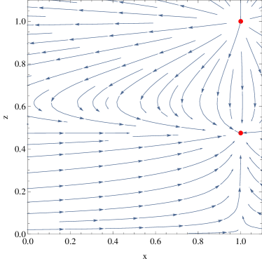
Figure 1: The figure shows the phase space structure in the $u-v$ plane corresponding to the Case 1 ($\zeta=\zeta_{0}+\zeta_{1}\frac{\dot{a}}{a}+\zeta_{2}\frac{\ddot{a}}{\dot{a}}$). The critical point (1,1) in the upper right corner of the plot is a past attractor and the point (1,0.475), below the first critical point, is a future attractor. The direction of the trajectories is shown by the arrow head.

$(u_{c},v_{c})$	$\lambda_{1}$	$\lambda_{2}$	Stability	$\omega$	$q$
$(1,1)$	3.9	3.4	Unstable, Past attractor	1.3	2.4
$(1,0.475)$	-3.45	-3	Stable, future attractor	-1	-1

Table 2: Critical points for case 1, with $\zeta=\zeta_{0}+\zeta_{1}\frac{\dot{a}}{a}+\zeta_{2}\frac{\ddot{a}}{\dot{a}}$

3.2.2 Case 2: with $\zeta=\zeta_{0}+\zeta_{1}\frac{\dot{a}}{a}$

Using the friedmann equations and conservation equation for matter we get the autonomous equation for this case as,

$$\begin{split}u^{\prime}&=\left(1-u\right)\left(\frac{\tilde{\zeta}_{0}}{v}+\tilde{\zeta}_{1}-\tilde{\zeta}_{0}\right)\\ v^{\prime}&=\frac{1}{2}\left(1-v\right)\left(\tilde{\zeta}_{0}+\left(\tilde{\zeta}_{1}-\tilde{\zeta}_{0}-3\right)v\right).\end{split}$$ (31)

In this case also there are two critical points $(u_{c},v_{c})=(1,1)$ and $(1,\frac{\tilde{\zeta}_{0}}{\tilde{\zeta}_{0}-\tilde{\zeta}_{1}+3})$. There properties are discussed below:

1. $(u_{c},v_{c})=(1,1)$
   This is a matter dominated solution representing the initial singular state, since $v=1$ implies $H\rightarrow\infty$. The critical point is same as that in case 1. The eigen values of the corresponding Jacobian matrix are,

   $$\lambda_{1}=\frac{3-\tilde{\zeta}_{1}}{2}=3.455,\ \ \ \ \lambda_{2}=-\tilde{\zeta}_{1}=3.91$$ (32)

   Since the eigen values are all positive, the critical point is an unstable node or can be called as the past attractor. Thus it is a source point of any orbit in the phase space. Using the values of bulk viscous parameters from table  1, we get $\omega=1.3$ and $q=2.45$ from Eqs. (26) and (25), respectively. From these values it is clear that the point represent a decelerated phase of the universe.

2. $(u_{c},v_{c})=(1,\frac{\tilde{\zeta}_{0}}{\tilde{\zeta}_{0}-\tilde{\zeta}_{1}+3})=(1,0.475)$
   The eigen values of the corresponding Jacobian matrix are,

   $$\lambda_{1}=\frac{\tilde{\zeta}_{1}-3}{2}=-3.455,\ \ \ \ \ \ \ \ \ \ \lambda_{2}=-3,$$ (33)

   using the value of $\tilde{\zeta}_{1}$ from Table  1. Since the eigen values are negative, this solution is a stable node and a future attractor. So all trajectories in the phase space tends to meet at this point. The equation of state parameter $\omega$ and the deceleration parameter $q$ are both found to be -1, thereby representing a de Sitter epoch.

The phase plot of this case is shown in Fig.  2. The phase space trajectories starts from the critical point (1,1) and ends in the point (1,0.475) in the u-v phase plane. The behaviour is same as that in the first case. The results are summarized in table  3.

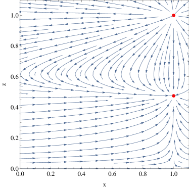
Figure 2: The figure shows the phase space structure in the $u-v$ plane corresponding to the Case 2 ($\zeta=\zeta_{0}+\zeta_{1}\frac{\dot{a}}{a}$). The critical point (1,1) in the upper right corner of the plot is a past attractor and the point (1,0.475), below the first critical point, is a future attractor. The direction of the trajectories is shown by the arrow head.

$(u_{c},v_{c})$	$\lambda_{1}$	$\lambda_{2}$	Stability	$\omega$	q
$(1,1)$	3.45	3.9	Unstable, Past attractor	1.3	2.4
$(1,0.475)$	-3.45	-3	Stable, future attractor	-1	-1

Table 3: Critical points for case 2, with $\zeta=\zeta_{0}+\zeta_{1}\frac{\dot{a}}{a}$

3.2.3 Case 3: with $\zeta=\zeta_{0}$

In this case, the autonomous equation reduces to,

$$\begin{split}u^{\prime}&=\left(1-u\right)\left(\frac{\tilde{\zeta}_{0}}{v}-\tilde{\zeta}_{0}\right)\\ v^{\prime}&=\frac{1}{2}\left(1-v\right)\left(\tilde{\zeta}_{0}-\left(\tilde{\zeta}_{0}+3\right)v\right).\end{split}$$ (34)

There exists two critical points:

1. $(u_{c},v_{c})=(u,1)$
   Here we see that the $u$ coordinate is variable, which can assume any values ranging from 0 to 1, while $v$ coordinate is a constant having value 1. As a result the critical point will not be an isolated point (see Fig.  3). It represents an initial state of the universe since $H\rightarrow\infty$. The eigen values of the corresponding Jacobian matrix are,

   $$\lambda_{1}=\frac{3}{2}=1.5,\ \ \ \ \ \ \ \ \ \ \ \ \ \lambda_{2}=0$$ (35)

   Since these values are positive, it is unstable. The value of equation of state parameter and the deceleration parameter are $\omega=0$ and $q=0.5$. From these values it is clear that it represents a matter dominated decelerated phase of the universe. Unlike the other two cases, where the values of $\omega$ corresponds to a stiff fluid, here in this case the value of $\omega$ indicates the non-relativistic dark matter causing a usual decelerated phase.

2. $(u_{c},v_{c})=(1,\frac{\tilde{\zeta}_{0}}{\tilde{\zeta}_{0}+3})=(1,0.39)$
   This corresponds to a matter dominated universe with $\frac{H_{0}}{H}=1.564$, representing the future phase of the universe. The eigen values are,

   $$\lambda_{1}=-\frac{3}{2}=-1.5,\ \ \ \ \ \ \ \ \ \ \ \ \ \ \lambda_{2}=-3$$ (36)

   The point is stable since both the eigen values are negative. The values of the equation of state parameter and the deceleration parameter are $\omega\sim-1$ and $q\sim-1$, which corresponds to a de Sitter phase.

The phase plot diagram is shown in Fig.  3. From the figure it is clear that the phase space trajectories originate from the non-isolated critical point (or rather a critical line), which is a past attractor (representing the matter dominated decelerated epoch of the universe). These trajectories finally converge to the stable critical point (1,0.39), representing the de-sitter phase. This is similar to the behaviour of the $\Lambda$CDM model. The results of the phase space analysis of the model are summarized in table  4.

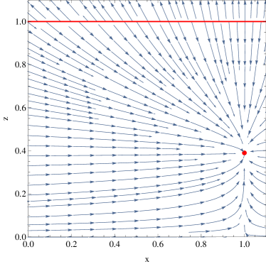
Figure 3: The figure shows the phase space structure in the $u-v$ plane corresponding to the Case 3 ($\zeta=\zeta_{0}$). The direction of the trajectories is shown by the arrow head.

$(u_{c},v_{c})$	$\lambda_{1}$	$\lambda_{2}$	Stability	$\omega$	q
$(u,1)$	1.5	0	Unstable, Past attractor	0	0.5
$(1,0.39)$	-1.5	-3	Stable, future attractor	-1	-1

Table 4: Critical points for case 3, with $\zeta=\zeta_{0}$

4 Universe with bulk viscous matter and radiation

The realistic picture of the universe have a radiation dominated phase followed by matter dominated epoch and a late accelerated epoch. Inorder to know whether the bulk viscous model predicts a prior radiation dominated phase, we study the phase space structure of the model by including radiation as an additional cosmic component. For such a universe, the friedmann equations becomes,

$$H^{2}=\frac{\rho_{m}+\rho_{r}}{3}$$ (37)

$$2\dot{H}+3H^{2}=HH_{0}\tilde{\zeta}-\frac{\rho_{r}}{3}$$ (38)

The conservation equation for matter is given by Eq. (11) and for radiation it is,

$$\dot{\rho_{r}}+4H\rho_{r}=0.$$ (39)

Eq. (38) can be modified using the radiation density parameter $\Omega_{r}=\frac{\rho_{r}}{3H^{2}}$, then the derivative of $H$ with respect to time $t$ becomes

$$\dot{H}=\frac{1}{2}\left(HH_{0}\tilde{\zeta}-3H^{2}-\Omega_{r}H^{2}\right)$$ (40)

Substituting this in Eq. (6), the total dimensionless bulk viscous parameter $\tilde{\zeta}$ takes the form,

$$\tilde{\zeta}=\frac{1}{2-\tilde{\zeta}_{2}}\left[2\tilde{\zeta}_{0}+\left(2\tilde{\zeta}_{1}-\tilde{\zeta}_{2}-\tilde{\zeta}_{2}\Omega_{r}\right)\frac{H}{H_{0}}\right],$$ (41)

which will reduces to Eq. (12) for $\Omega_{r}=0$. The deceleration parameter $q$ and equation of state parameter $\omega$ can be obtained by substituting Eqs. (40) and (41) in Eqs. (13) and (14) as

$$q=\frac{1}{2-\tilde{\zeta}_{2}}\left(1-\tilde{\zeta}_{1}+\Omega_{r}-\tilde{\zeta}_{0}(\frac{H_{0}}{H})\right)$$ (42)

$$\omega=\frac{1}{3(2-\tilde{\zeta}_{2})}\left(2\Omega_{r}-2\tilde{\zeta}_{1}+\tilde{\zeta}_{2}-2\tilde{\zeta}_{0}(\frac{H_{0}}{H})\right]$$ (43)

which are reducing to Eqs. (15) and (16) for $\Omega_{r}=0$. In the radiation dominated case (i.e., when $\Omega_{r}\rightarrow 1$, then $\frac{H_{0}}{H}\rightarrow 0$), the deceleration parameter and the equation of state reduces to,

$$q\sim\frac{2-\tilde{\zeta}_{1}}{2-\tilde{\zeta}_{2}}$$ (44)

$$\omega\sim\frac{2-2\tilde{\zeta}_{1}+\tilde{\zeta}_{2}}{3(2-\tilde{\zeta}_{2})}$$ (45)

When radiation is the dominant component,universe there would be no acceleration in expansion such that $q>0$ and $\omega>-\frac{1}{3}$. These conditions constrains the bulk viscous parameters as $\tilde{\zeta}_{1}<2$ and $\tilde{\zeta}_{2}<2$. In the extreme limit corresponding to the radiation dominated phase, $q=1$ and $\omega=\frac{1}{3}$ and is corresponding to $\tilde{\zeta}_{1}=\tilde{\zeta}_{2}$.

4.1 Phase space analysis

For doing the phase space analysis, we are defining the phase space co-ordinates as

$$\begin{split}u&=\Omega_{m}=\frac{\rho_{m}}{3H^{2}}\\ y&=\Omega_{r}=\frac{\rho_{r}}{3H^{2}}\\ v&=\frac{1}{\frac{H_{0}}{H}+1}\end{split}$$ (46)

Contrary to the previous discussion, here we take $\zeta=\zeta_{0}$ as Case 1,$\zeta=\zeta_{0}+\zeta_{1}\frac{\dot{a}}{a}$ as Case 2 and $\zeta=\zeta_{0}+\zeta_{1}\frac{\dot{a}}{a}+\zeta_{2}\frac{\ddot{a}}{\dot{a}}$ as Case 3.

4.1.1 Case 1: with $\zeta=\zeta_{0}$

Using Eqs. (11), (39) and (40), the autonomous equations satisfied by the phase space co-ordinates becomes,

$$\begin{split}u^{\prime}&=\tilde{\zeta}_{0}(1-u)(\frac{1-v}{v})+uy\\ y^{\prime}&=\frac{y}{v}\left(\tilde{\zeta}_{0}(v-1)+v(y-1)\right)\\ v^{\prime}&=\frac{(1-v)}{2}\left(\tilde{\zeta}_{0}(1-v)-v(y+3)\right)\end{split}$$ (47)

The Jacobian matrix for this can be obtained from Eq. (56) by setting $\tilde{\zeta}_{1}=\tilde{\zeta}_{2}=0$. The critical points are,

1. $(u_{c},y_{c},v_{c})=(0,1,1)$
   This corresponds to the radiation dominated phase of the universe. The eigen values of the corresponding Jacobian matrix are,

   $$\lambda_{1}=1,\ \ \ \lambda_{2}=1,\ \ \ \lambda_{3}=2.$$ (48)

   All the eigen values are positive, indicating an unstable node (past attractor). The equation of state parameter and the deceleration parameter corresponding to this critical point can be obtained by substituting the values of $u_{c}$, $y_{c}$ and $v_{c}$ in Eqs. (43) and (42), respectively, and are found to be $\omega=\frac{1}{3}$ and $q=1$. These values confirms that the point is the radiation dominated phase of the universe.

2. $(u_{c},y_{c},v_{c})=(u,0,1)$
   The eigen values of the corresponding Jacobian matrix are,

   $$\lambda_{1}=-1,\ \ \ \lambda_{2}=0,\ \ \ \lambda_{3}=\frac{3}{2}$$ (49)

   These values shows that the point is a saddle point. The equation of state parameter and deceleration parameter are found to be, $\omega=0$ and $q=\frac{1}{2}$ respectively from Eqs. (43) and (42), indicating that the universe is matter dominated without accelerating, hence $u_{c}\sim 1$.

3. $(u_{c},y_{c},v_{c})=(1,0,\frac{\tilde{\zeta}_{0}}{\tilde{\zeta}_{0}+3})$
   The eigen values of the corresponding Jacobian matrix are,

   $$\lambda_{1}=-4,\ \ \ \lambda_{2}=-3,\ \ \ \lambda_{3}=-\frac{3}{2}$$ (50)

   The critical point is a stable node, since all the eigen values are negative.From Eqs. (43) and (42), the equation of state parameter, $\omega=-1$ and deceleration parameter $q=-1$, independent of the value of $\tilde{\zeta}_{0}$. This represent a de Sitter type phase.

Thus this case predicts a universe beginning with a radiation dominated phase (past attractor) and then transit to a decelerated matter dominated phase (saddle point) and then finally evolving to a de Sitter type universe (stable future attractor). Thus it has a close resemblance with the conventional evolution of the universe. The results are summarized in Table  5.

$(u_{c},y_{c},v_{c})$	$\lambda_{1}$	$\lambda_{2}$	$\lambda_{3}$	Stability	$\omega$	q
$(0,1,1)$	1	1	2	Unstable node	$\frac{1}{3}$	1
$(u,0,1)$	-1	0	$\frac{3}{2}$	Saddle	0	$\frac{1}{2}$
$(1,0,\frac{\tilde{\zeta}_{0}}{\tilde{\zeta}_{0}+3)})$	-4	-3	$-\frac{3}{2}$	Stable node	-1	-1

Table 5: Critical points for Case 1: with $\zeta=\zeta_{0}$

4.1.2 Case 2: with $\zeta=\zeta_{0}+\zeta_{1}\frac{\dot{a}}{a}$

In this case the autonomous equations are,

$$\begin{split}u^{\prime}&=\frac{\tilde{\zeta}_{0}(1-u)}{v}+(1-u)(\tilde{\zeta}_{1}-\tilde{\zeta}_{0})+uy\\ y^{\prime}&=y\left(\frac{\tilde{\zeta}_{0}(v-1)}{v}+y-1-\tilde{\zeta}_{1}\right)\\ v^{\prime}&=\frac{1}{2-\tilde{\zeta}_{2}}\left(1-v\right)\left(\tilde{\zeta}_{0}(1-v)+(\tilde{\zeta}_{1}-3-y)v\right)\end{split}$$ (51)

The Jacobian matrix for this autonomous system is given by Eq. (56) provided $\tilde{\zeta}_{2}=0$. The critical points are,

1. $(u_{c},y_{c},v_{c})=(-\tilde{\zeta}_{1},\tilde{\zeta}_{1}+1,1)$
   The eigen values of the corresponding Jacobian matrix are,

   $$\lambda_{1}=\tilde{\zeta}_{1}+1,\ \lambda_{2}=1,\ \lambda_{3}=2.$$ (52)

   The point will be unstable node if $\tilde{\zeta}_{1}>-1$, otherwise it will be a saddle point. The equation of state parameter, $\omega=\frac{1}{3}$ and deceleration parameter $q=1$, independent of $\tilde{\zeta}_{0}$ and $\tilde{\zeta}_{1}$. Hence if $\tilde{\zeta}_{1}=0$, the point will indicate an exact radiation dominated universe.

2. $(u_{c},y_{c},v_{c})=(1,0,1)$
   This corresponds to a matter dominated initial stage of the universe. The eigen values of the corresponding Jacobian matrix are,

   $$\lambda_{1}=-(\tilde{\zeta}_{1}+1),\ \lambda_{2}=-\tilde{\zeta}_{1},\ \lambda_{3}=\frac{3-\tilde{\zeta}_{1}}{2}.$$ (53)

   The point will be unstable node if $\tilde{\zeta}_{1}<-1$, a stable one if $\tilde{\zeta}_{1}>3$ and a saddle point otherwise. For this point, the equation of state, $\omega=-\frac{\tilde{\zeta}_{1}}{3}$ and the deceleration parameter $q=\frac{1-\tilde{\zeta}_{1}}{2}$. If $\tilde{\zeta}_{1}<-1$, then the values of $\omega$ and $q$ will not represent a conventional matter dominated universe. So only if $\tilde{\zeta}_{1}=0$, this will represent a conventional matter dominated universe without acceleration.

3. $(u_{c},y_{c},v_{c})=(1,0,\frac{\tilde{\zeta}_{0}}{\tilde{\zeta}_{0}-(\tilde{\zeta}_{1}-3)})$
   The eigen values are,

   $$\lambda_{1}=-4,\ \lambda_{2}=-3,\ \lambda_{3}=\frac{1}{2}(\tilde{\zeta}_{1}-3).$$ (54)

   The point will be a stable one if $\tilde{\zeta}_{1}<3$, otherwise it will be a saddle point. The equation of state parameter, $\omega=-1$ and deceleration parameter $q=-1$, independent of the values of viscous parameters, representing a de Sitter type universe. So If $\tilde{\zeta}_{1}=0$, the point will be represent a stable future attractor with same values of $\omega$ and $q$.

In order to represent a realistic picture, the first critical point must be a unstable (past attractor) radiation dominated phase, the second must be a matter dominated phase without acceleration (saddle point) and the third must corresponds to the stable accelerated phase of the universe. Inorder to satisfy this, $\tilde{\zeta}_{1}$ should be equal to zero. The results of the analysis is given in Table  6

$(u_{c},y_{c},v_{c})$	$\lambda_{1}$	$\lambda_{2}$	$\lambda_{3}$	Stability	$\omega$	q
$(-\tilde{\zeta}_{1},\tilde{\zeta}_{1}+1,1)$	$\tilde{\zeta}_{1}+1$	1	2	Unstable node if $\tilde{\zeta}_{1}>-1$, otherwise a saddle point	$\frac{1}{3}$	1
$(1,0,1)$	$-(\tilde{\zeta}_{1}+1)$	$-\tilde{\zeta}_{1}$	$\frac{3-\tilde{\zeta}_{1}}{2}$	Unstable node if $\tilde{\zeta}_{1}<-1$, Stable if $\tilde{\zeta}_{1}>3$, a saddle point otherwise	$\frac{-\tilde{\zeta}_{1}}{3}$	$\frac{1-\tilde{\zeta}_{1}}{2}$
$(1,0,\frac{\tilde{\zeta}_{0}}{\tilde{\zeta}_{0}-(\tilde{\zeta}_{1}-3)})$	-4	-3	$\frac{1}{2}(\tilde{\zeta}_{1}-3)$	Unstable node if $\tilde{\zeta}_{1}<3$, otherwise a saddle point	-1	-1

Table 6: Critical points for Case 2: with $\zeta=\zeta_{0}+\zeta_{1}\frac{\dot{a}}{a}$

4.1.3 Case 3: with $\zeta=\zeta_{0}+\zeta_{1}\frac{\dot{a}}{a}+\zeta_{2}\frac{\ddot{a}}{\dot{a}}$

In this case the phase space variables satisfy the autonomous equations,

$$\begin{split}u^{\prime}=&\frac{1}{v(2-\tilde{\zeta}_{2})}(2\tilde{\zeta}_{0}(1-u)(1-v)+\\ &v((u-y-1)\tilde{\zeta}_{2}+2(1-u)\tilde{\zeta}_{1}+2yu))\\ y^{\prime}=&\frac{1}{v(2-\tilde{\zeta}_{2})}2y\left(\tilde{\zeta}_{0}(v-1)+(y-1-\tilde{\zeta}_{1}+\tilde{\zeta}_{2})v\right)\\ v^{\prime}=&\frac{1}{2-\tilde{\zeta}_{2}}\left(1-v\right)\left(\tilde{\zeta}_{0}(1-v)+(\tilde{\zeta}_{1}+\tilde{\zeta}_{2}-3-y)v\right)\end{split}$$ (55)

$(u_{c},y_{c},v_{c})$	$\lambda_{1}$	$\lambda_{2}$	$\lambda_{3}$	Stability	$\omega$	q
$(\tilde{\zeta}_{2}-\tilde{\zeta}_{1},1-(\tilde{\zeta}_{2}-\tilde{\zeta}_{1},1)$	$\frac{-2(\tilde{\zeta}_{1}-\tilde{\zeta}_{2}+1)}{\tilde{\zeta}_{2}-2}$	1	2	Unstable node if $\tilde{\zeta}_{2}<2$, Saddle point otherwise	$\frac{1}{3}$	1
$(1,0,1)$	$\frac{2(\tilde{\zeta}_{1}-\tilde{\zeta}_{2}+1)}{\tilde{\zeta}_{2}-2}$	$\frac{2\tilde{\zeta}_{1}-\tilde{\zeta}_{2}}{\tilde{\zeta}_{2}-2}$	$\frac{\tilde{\zeta}_{1}+\tilde{\zeta}_{2}-3}{\tilde{\zeta}_{2}-2}$	Unstable node if (i) $\tilde{\zeta}_{2}>2,\tilde{\zeta}_{1}>1,\tilde{\zeta}_{1}-\tilde{\zeta}_{2}>-1$, (ii) $\tilde{\zeta}_{2}<2,\tilde{\zeta}_{1}<1,\tilde{\zeta}_{1}-\tilde{\zeta}_{2}<-1$	$\frac{-2\tilde{\zeta}_{1}+\tilde{\zeta}_{2}}{3(2-\tilde{\zeta}_{2})}$	$\frac{1-\tilde{\zeta}_{1}}{2-\tilde{\zeta}_{2}}$
$(1,0,\frac{\tilde{\zeta}_{0}}{\tilde{\zeta}_{0}-(\tilde{\zeta}_{1}+\tilde{\zeta}_{2}-3)})$	-4	-3	$-\frac{\tilde{\zeta}_{1}+\tilde{\zeta}_{2}-3}{\tilde{\zeta}_{2}-2}$	Stable node if (i) $\tilde{\zeta}_{0}>0,\tilde{\zeta}_{2}<2$, (ii) $\tilde{\zeta}_{0}<0,\tilde{\zeta}_{2}>2$, Saddle point otherwise	-1	-1

Table 7: Critical points for Case 3: with $\zeta=\zeta_{0}+\zeta_{1}\frac{\dot{a}}{a}+\zeta_{2}\frac{\ddot{a}}{\dot{a}}$

When $\tilde{\zeta}_{1}=\tilde{\zeta}_{2}=0$, the critical point corresponds to $w=0$, $q=\frac{1}{2}$ implying a matter dominated universe without acceleration.

The Jacobian matrix for these set of autonomous equation is given by,

$$\begin{bmatrix}\left(\frac{2\tilde{\zeta}_{0}(1-v)+(2\tilde{\zeta}_{1}-\tilde{\zeta}_{2}-2y)v}{(\tilde{\zeta}_{2}-2)v}\right)_{0}&\left(\frac{\tilde{\zeta}_{2}-2u}{\tilde{\zeta}_{2}-2}\right)_{0}&\left(\frac{2\tilde{\zeta}_{0}(1-u)}{(\tilde{\zeta}_{2}-2)v^{2}}\right)_{0}\\ 0&\left(\frac{2(\tilde{\zeta}_{0}-\tilde{\zeta}_{0}v+(1+\tilde{\zeta}_{1}-\tilde{\zeta}_{2}-2y)v)}{(\tilde{\zeta}_{2}-2)v}\right)_{0}&\left(\frac{-2\tilde{\zeta}_{0}y}{(\tilde{\zeta}_{2}-2)v^{2}}\right)_{0}\\ 0&\left(\frac{(1-v)v}{\tilde{\zeta}_{2}-2}\right)_{0}&\left(\frac{2\tilde{\zeta}_{0}(1-v)+(\tilde{\zeta}_{1}+\tilde{\zeta}_{2}-3-y)(2v-1)}{\tilde{\zeta}_{2}-2}\right)_{0}\end{bmatrix}$$ (56)

The critical points $(u_{c},y_{c},v_{c})$ of these equations are

1. $(u_{c},y_{c},v_{c})=(\tilde{\zeta}_{2}-\tilde{\zeta}_{1},1-(\tilde{\zeta}_{2}-\tilde{\zeta}_{1}),1)$
   For this solution to represent the realistic phase (for example, matter dominated or radiation dominated) of the universe, the bulk viscous parameters should satisfy the condition, $0\leq\tilde{\zeta}_{2}-\tilde{\zeta}_{1}\leq 1$. The eigen values of the corresponding Jacobin matrix are,

   $$\lambda_{1}=\frac{-2(\tilde{\zeta}_{1}-\tilde{\zeta}_{2}+1)}{\tilde{\zeta}_{2}-2},\ \ \ \lambda_{2}=1,\ \ \ \lambda_{3}=2.$$ (57)

   The point will be unstable if $\tilde{\zeta}_{2}-2<0$ and a saddle point otherwise. The equation of state parameter and deceleration parameter corresponding to this critical point are, $\omega=\frac{1}{3}$ and $q=1$.

2. $(u_{c},y_{c},v_{c})=(1,0,1)$
   This point corresponds to a matter dominated phase of the universe. The eigen values of the corresponding jacobian matrix are,

   $$\lambda_{1}=\frac{2(\tilde{\zeta}_{1}-\tilde{\zeta}_{2}+1)}{\tilde{\zeta}_{2}-2},\lambda_{2}=\frac{2\tilde{\zeta}_{1}-\tilde{\zeta}_{2}}{\tilde{\zeta}_{2}-2},\lambda_{3}=\frac{\tilde{\zeta}_{1}+\tilde{\zeta}_{2}-3}{\tilde{\zeta}_{2}-2}.$$ (58)

   This critical point will be unstable if (i) $\tilde{\zeta}_{2}>2,\tilde{\zeta}_{1}>1,\tilde{\zeta}_{1}-\tilde{\zeta}_{2}>-1$ or if (ii) $\tilde{\zeta}_{2}<2,\tilde{\zeta}_{1}<1,\tilde{\zeta}_{1}-\tilde{\zeta}_{2}<-1$. The equation of state parameter and the deceleration parameter corresponding to this critical point are, $\omega=\frac{2\tilde{\zeta}_{1}-\tilde{\zeta}_{2}}{3(\tilde{\zeta}_{2}-2)}$ and $q=\frac{\tilde{\zeta}_{1}-1}{\tilde{\zeta}_{2}-2}$.

3. $(u_{c},y_{c},v_{c})=(1,0,\frac{\tilde{\zeta}_{0}}{\tilde{\zeta}_{0}-(\tilde{\zeta}_{1}+\tilde{\zeta}_{2}-3)})$
   This also represents a matter dominated universe with $\frac{H_{0}}{H}=\frac{3-(\tilde{\zeta}_{1}+\tilde{\zeta}_{2})}{\tilde{\zeta}_{0}}$. The eigen values of the Jacobian matrix are,

   $$\lambda_{1}=-4,\ \ \ \lambda_{2}=-3,\ \ \ \lambda_{3}=-\frac{\tilde{\zeta}_{1}+\tilde{\zeta}_{2}-3}{\tilde{\zeta}_{2}-2}.$$ (59)

   The relation $\frac{H_{0}}{H}=\frac{3-(\tilde{\zeta}_{1}+\tilde{\zeta}_{2})}{\tilde{\zeta}_{0}}>0$ holds if $\tilde{\zeta}_{0}>0$ and $\tilde{\zeta}_{1}+\tilde{\zeta}_{2}<3$ or if $\tilde{\zeta}_{0}<0$ and $\tilde{\zeta}_{1}+\tilde{\zeta}_{2}>3$. Applying this condition to the eigen value $\lambda_{3}$ we find that this critical point will be stable (or future attractor) if (i) $\tilde{\zeta}_{2}<2$ for $\tilde{\zeta}_{0}>0$ or if (ii) $\tilde{\zeta}_{2}>2$ for $\tilde{\zeta}_{0}<0$. It is a saddle point otherwise. The equation of state parameter, $\omega=-1$ and deceleration parameter $q=-1$ implies a de sitter like universe.

The above critical points would represent the realistic evolution of the universe, if, successively, the first critical point is a radiation dominated one, the second one is a matter dominated phase without acceleration and the last one be a matter dominated phase with acceleration. For this, first of all the values of the viscous coefficients must be such that $\tilde{\zeta}_{1}\sim\tilde{\zeta}_{2}$. Under this conditions the critical points becomes

1. $(u_{c},y_{c},v_{c})=(0,1,1)$, corresponding to radiation dominated phase with $\omega=\frac{1}{3}$ and $q=1$

2. $(u_{c},y_{c},v_{c})=(1,0,1)$, corresponding to matter dominated phase with $\omega=\frac{\tilde{\zeta}_{2}}{3(\tilde{\zeta}_{2}-2)}$ and $q=\frac{\tilde{\zeta}_{2}-1}{\tilde{\zeta}_{2}-2}$

3. $(u_{c},y_{c},v_{c})=(1,0,\frac{\tilde{\zeta}_{0}}{\tilde{\zeta}_{0}-(2\tilde{\zeta}_{2}-3)})$, corresponding to accelerating phase with $\omega=-1$ and $q=-1$.

Then by analyzing the eigen values, it is found that the first critical point (Eq.(57)) will be a past attractor if $\tilde{\zeta}_{2}<2$. Under this condition, the second critical point, given by Eq. (58), corresponding to the matter dominated phase, will be a saddle point. The third critical point, corresponding to the accelerated phase, will be a stable one if $\tilde{\zeta}_{2}<\frac{3}{2}$. However, under this condition, there is a chance for $\omega$ and $q$ to become negative in the case of matter dominated phase corresponding to second set of critical points (58). This doesn’t represent a conventional matter dominated phase of the universe. For this critical point to represent a matter dominated phase without acceleration, it requires $\omega=0$ and $q=\frac{1}{2}$. This is possible only if $\tilde{\zeta}_{1}\simeq\tilde{\zeta}_{2}=0$. Due to this conditions, the nature of the first and the last critical points will not be affected. i.e., the first critical point will be a radiation dominated past attractor, the second one will be an unaccelerated matter dominated saddle point and the third will be a stable node corresponding to a de Sitter phase. Thus it predicts a universe starting from a radiation dominated era and then entering a decelerated matter dominated phase and then finally evolving to the de Sitter universe.Thus we see that unless $\tilde{\zeta}_{1}=\tilde{\zeta}_{2}=0$, the model doesn’t predict a prior radiation dominated phase and a decelerated matter dominated phase of the universe. The results are summarized in Table  7

5 Conclusion

We have done the phase space analysis of the universe with bulk viscous matter having bulk viscous coefficient of the form (i)$\zeta=\zeta_{0}$, (ii) $\zeta=\zeta_{0}+\zeta_{1}\frac{\dot{a}}{a}$, (iii) $\zeta=\zeta_{0}+\zeta_{1}\frac{\dot{a}}{a}+\zeta_{2}\frac{\ddot{a}}{\dot{a}}$. First we have considered a universe containing bulk viscous matter alone and for the above cases, the value of the bulk viscous parameters are extracted using SCP ”Union” Type I a Supernova data. Using these the asymptotic properties of the model are studied and phase space for each cases are plotted. It is found that for all the three cases, it predicts a prior matter dominated universe without acceleration, which is an unstable node and a stable matter dominated universe with acceleration, similar to the de Sitter phase.

Secondly we consider a universe including radiation and bulk viscous matter to check whether it predicts a prior conventional radiation dominance also. The phase space analysis of the model is done for the three different cases separately. For the case $\zeta=\zeta_{0}$, it is found that it predicts a universe beginning with a radiation dominated phase (past attractor) and then transit to a decelerated matter dominated phase (saddle point) and then finally evolving to a de Sitter type universe (stable future attractor). The other two cases, i.e., with $\zeta=\zeta_{0}+\zeta_{1}\frac{\dot{a}}{a}$ and $\zeta=\zeta_{0}+\zeta_{1}\frac{\dot{a}}{a}+\zeta_{2}\frac{\ddot{a}}{\dot{a}}$, predicts a stable accelerated phase of the universe similar to a de Sitter type with $\omega=-1$ and $q=-1$. However, these doesn’t predicts a prior radiation dominated phase and conventional decelerated matter dominated phase of the universe, unless $\zeta_{1}=\zeta_{2}=0$. There are approaches in the literature  [29, 47, 48] where bulk viscosity is included through $\zeta=\alpha\rho^{m}$, but there is no guarantee that this approach will give the same result compared to the present case, for instant in reference  [55] it is shown that these two approaches are different in the structure formation

Thus, the bulk viscous model, which is an alternative to dark energy, will predicts all the conventional phases and evolution of the universe only with constant bulk viscous coefficient, $\zeta=\zeta_{0}$. For the other two cases, with $\zeta=\zeta_{0}+\zeta_{1}\frac{\dot{a}}{a}$ and $\zeta=\zeta_{0}+\zeta_{1}\frac{\dot{a}}{a}+\zeta_{2}\frac{\ddot{a}}{\dot{a}}$, even though explains the late acceleration of the universe  [36], but fails to predict the prior radiation dominated phase and the decelerated matter dominated phase of the universe.

Acknowledgment
The author (AS) is thankful to DST for giving financial support through INSPIRE fellowship. Author (TKM) is thankful to The Inter-University Centre for Astronomy and Astrophysics (IUCAA), Pune, India for the hospitality during the visits where part of the work has been carried out.

Appendix

1. Validity of Generalised second law for the present model
   In the FLRW space-time, the law of generation of the local entropy is given as [56]

   $$T\nabla_{\nu}s^{\nu}=\zeta(\nabla_{\nu}u^{\nu})^{2}=9H^{2}\zeta$$ (60)

   where $T$ is the temperature and $\nabla_{\nu}s^{\nu}$ is the rate of generation of entropy in unit volume. The second law of thermodynamics will be satisfied if,

   $$T\nabla_{\nu}s^{\nu}\geq 0$$ (61)

   which implies from equation (60) that

   $$\zeta\geq 0.$$ (62)

   For $\zeta=\zeta_{0}+\zeta_{1}\frac{\dot{a}}{a}+\zeta_{2}\frac{\ddot{a}}{\dot{a}}$, it is found that the total $\zeta$ is negative when $z>0.8$ [36], thereby violating local second law in the early universe. But when $\zeta=\zeta_{0}$, $\zeta$ always remains positive through out the evolution of the universe (since $\zeta_{0}>0$) and hence satisfying the local second law of thermodynamics.

   However, if one consider the Generalised second law (GSL) which includes the total entropy of the universe plus that of the horizon, it is found that total entropy is always on the increase for total $\zeta$, if apparent horizon is considered as the boundary [36]. On taking account of the validity of GSL, it can be reasonably argued that in the early universe where $\zeta$ becomes negative, the total pressure becomes positive and the viscous matter will act as an ordinary non-relativistic matter causing decelerated expansion. There are conventional dark energy models which act as the non-relativistic matter in the early phases causing decelerated expansion [57, 58, 59, 60]. There are also works [61, 62, 63, 64], showing that the entropy change can become negative depending on the equation of state of matter. In the current literature, there are publications dealing the problems with negative viscous coefficients [61]. In this reference the authors has point out that the positivity of $\zeta$ in conventional cosmology is based upon the requirement that the change of entropy in a non-equilibrium system is positive, and they argues that the possibility of allowing for negative values of $\zeta$ is not so unreasonable in view of the general bizarre properties of the dark energy fluid, as far as temperature is positive. Apart from this our model also satisfies GSL with total $\zeta$.

   Now we will consider event horizon as the boundary for analyzing the validity of GSL for $\zeta=\zeta_{0}$. The radius of the event horizon is given as,

   $$R_{E}=a\int_{a}^{\infty}\frac{da}{Ha^{2}}$$ (63)

   where $a$ is the scale factor and $H$ is the Hubble parameter given as [36],

   $$H(a)=H_{0}\left[a^{-\frac{3}{2}}\left(1-\frac{\tilde{\zeta}_{0}}{3}\right)+\frac{\tilde{\zeta}_{0}}{3}\right]$$ (64)

   $H_{0}$ is the present value of the Hubble parameter. The radius of the event horizon then obtained as,

   $$\begin{split}R_{E}=\frac{a}{H_{0}}(4.16+2.65\arctan[0.58-1.4\sqrt{a}]-1.53\log[0.97+1.18\sqrt{a}]\\ +0.76\log[0.94-1.14\sqrt{a}+1.38a])\end{split}$$ (65)

   The entropy associated with the event horizon is

   $$S_{E}=\frac{A}{4}$$ (66)

   $A=4\pi{R_{E}}^{2}$ is the area of the horizon. So entropy becomes

   $$S_{E}=\pi{R_{E}}^{2}$$ (67)

   The temperature of the event horizon can be defined as $T_{E}=\frac{1}{2\pi R_{E}}$. Using these we get[65],

   $$T_{E}\dot{S}_{E}=\dot{R}_{E}=HR_{E}-1$$ (68)

   The entropy of matter can be obtained using the Gibb’s relation,

   $$\begin{split}T_{m}dS_{m}=&d(\rho_{m}V)+PdV\\ =&(\rho_{m}+P)dV+Vd\rho_{m}\end{split}$$ (69)

   where $T_{m}$ is the temperature of the bulk viscous matter, $V=\frac{4}{3}\pi R_{E}^{3}$ is the volume enclosed by the event horizon. Using the expression for pressure $P=-3H\zeta_{0}=HH_{0}\tilde{\zeta}_{0}$ ($\tilde{\zeta}_{0}=\frac{3\zeta}{H_{0}}$ is the dimensionless viscous parameter), the conservation equation and the relation $\dot{R}_{E}=HR_{E}-1$ , we get

   $$T_{m}\dot{S}_{m}=4\pi R_{E}^{2}(HH_{0}\tilde{\zeta_{0}}-3H^{2})$$ (70)

   Under equilibrium conditions, the temperature $T_{m}$ of the viscous matter and that of the horizon $T_{E}$ are equal, $T_{m}=T_{E}=T$. Adding Eqs. (68) and (70), we get,

   $$T(\dot{S}_{E}+\dot{S}_{m})=4\pi R_{E}^{2}(HH_{0}\tilde{\zeta_{0}}-3H^{2})+HR_{E}-1$$ (71)

   For GSL to be valid, $T(\dot{S}_{E}+\dot{S}_{m})>0$. We have check the validity by numerically plotting Eq. (71) with respect to $a$ and is shown in the figure 4.

   

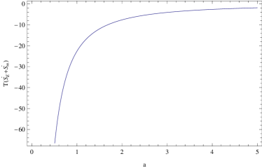
   Figure 4: Plot of $T(\dot{S}_{E}+\dot{S}_{m})$ with respect to the scale factor $a$.

   The plot shows that the GSL is violated when we take event horizon as the boundary. So, in our model GSL is satisfied at the apparent horizon but violated at the event horizon. At this juncture, one may note that a more novel GSL was proposed by Bousso et.al [66] regardless of whether an event horizon is present. However, the validity of this new GSL is to checked for our model

   There are many works in literature in tune with our result regarding the validity of GSL. In references [67, 69], the authors have shown that in general, for an accelerating universe, GSL of thermodynamics holds only in the case where the enveloping surface is the apparent horizon, but not in the case of the event horizon. There are also many other dark energy models which shows the same behavior. Some models are viscous model [68, 70], interacting dark energy model with dark matter [65], Holographic Ricci dark energy model [71, 72], DGP model [73], braneworld model [74]. In all these references, it is found that the event horizon in an accelerating universe is not a boundary from the thermodynamical point of view. In lieu of these, apparent horizon can be considered as the proper thermodynamic boundary.

2. Statefinder parameter diagnostic for $\zeta=\zeta_{0}$ (comparison with $\Lambda$CDM model)
   For comparison we have make use of the statefinder parameter diagnostic introduced by Sahni et al [75]. The statefinder parameters $\{r,s\}$ are defined as,

   $$r=\frac{\dddot{a}}{aH^{3}},\ \ \ \ \ \ s=\frac{r-1}{3\left(q-\frac{1}{2}\right)}.$$ (72)

   In terms of $h=\frac{H}{H_{0}}$, $r$ and $s$ can be written as

   $$r=\frac{1}{2h^{2}}\frac{d^{2}h^{2}}{dx^{2}}+\frac{3}{2h^{2}}\frac{dh^{2}}{dx}+1$$ (73)

   $$s=-\frac{\frac{1}{2h^{2}}\frac{d^{2}h^{2}}{dx^{2}}+\frac{3}{2h^{2}}\frac{dh^{2}}{dx}}{\frac{3}{2h^{2}}\frac{dh^{2}}{dx}+\frac{9}{2}}.$$ (74)

   Using the expression for $h$ from Eq. (64) for $\zeta=\zeta_{0}$, these parameters become,

   $$\begin{split}r=\frac{3(\tilde{\zeta}_{0}-3)}{4h^{2}}a^{-\frac{3}{2}}[\frac{\tilde{\zeta}_{0}}{3}-2h]+\frac{3(\tilde{\zeta}_{0}-3)}{2h}a^{-\frac{3}{2}}+1\end{split}$$ (75)

   $$s=-\frac{\frac{3(\tilde{\zeta}_{0}-3)}{4h^{2}}a^{-\frac{3}{2}}[\frac{\tilde{\zeta}_{0}}{3}-2h]+\frac{3(\tilde{\zeta}_{0}-3)}{2h}a^{-\frac{3}{2}}}{\frac{3(\tilde{\zeta}_{0}-3)}{2h}a^{-\frac{3}{2}}+\frac{9}{2}}.$$ (76)

   The $\{r,s\}$ plane trajectory of the model with $\zeta=\zeta_{0}$ is shown in figure 5.

   

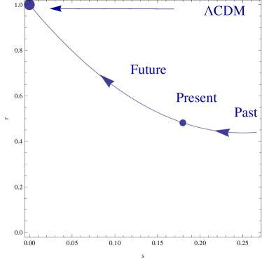
   Figure 5: The evolution of the model in the r-s plane for the best estimates of the parameter $\tilde{\zeta}_{0}$

   The plot lie in the region $r<1,s>0$, which is the general behavior of any quintessence model.

References

- [1] A. G. Riess et al., Observational Evidence from Supernovae for an Accelerating Universe and a Cosmological Constant, Astron. J. 116 (1998) 1009.
- [2] S. Perlmutter et al., Measurements of and from 42 High-Redshift Supernovae, Astrophys. J. 517 (1999) 565.
- [3] C. L. Bennett et al., First-Year Wilkinson Microwave Anisotropy Probe (WMAP) Observations: Preliminary Maps and Basic Results, Astrophys. J. Suppl. Ser. 148 (2003) 1.
- [4] Tegmark et al., Cosmological parameters from SDSS and WMAP, Phys. Rev. D 69 (2004) 103501.
- [5] Seljak et al., Cosmological parameter analysis including SDSS Ly forest and galaxy bias: Constraints on the primordial spectrum of fluctuations, neutrino mass, and dark energy, Phys. Rev. D 71 (2005) 103515.
- [6] E. Komatsu et al., Seven-year Wilkinson Microwave Anisotropy Probe (WMAP) Observations: Cosmological Interpretation, Astrophys. J. Suppl. Ser. 192 (2011) 18.
- [7] Steven Weinberg, The cosmological constant problem, Rev. Mod. Phys. 61 (1989) 1.
- [8] Edmund J Copeland, M. Sami and S. Tsujikawa, Dynamics of dark energy, Int. J. Mod Phys D 15 (2006) 1753.
- [9] Yasunori Fujii, Origin of the gravitational constant and particle masses in a scale-invariant scalar-tensor theory, Phys. Rev. D 26 (1982) 2580.
- [10] Sean M. Carroll, Quintessence and the Rest of the World: Suppressing Long-Range Interactions, Phys. Rev. Lett. 81 (1998) 3067.
- [11] L. H. Ford, Cosmological-constant damping by unstable scalar fields, Phys. Rev. D 35 (1987) 2339.
- [12] Edmund J. Copeland and Andrew R. Liddle and David Wands, Exponential potentials and cosmological scaling solutions, Phys. Rev. D 57 (1998) 4686.
- [13] Takeshi Chiba, Takahiro Okabe and Masahide Yamaguchi, Kinetically driven quintessence, Phys. Rev. D 62 (2000) 023511.
- [14] C. Armendariz-Picon, V. Mukhanov and Paul J. Steinhardt, Dynamical Solution to the Problem of a Small Cosmological Constant and Late-Time Cosmic Acceleration, Phys. Rev. Lett. 85 (2000) 4438.
- [15] Alexander Kamenshchik, Ugo Moschella and Vincent Pasquier, An alternative to quintessence, Phys. Lett. B 511 (2001) 265.
- [16] M. C. Bento, O. Bertolami and A. A. Sen, Generalized Chaplygin gas, accelerated expansion, and dark-energy-matter unification, Phys. Rev. D 66 (2002) 043507.
- [17] Salvatore Capozziello, Curvature quintessence, Int. J. Mod Phys D 11 (2002) 483.
- [18] Thomas P. Sotiriou and Valerio Faraoni, theories of gravity, Rev. Mod. Phys. 82 (2010) 451.
- [19] R. Ferraro and F. Fiorini, Modified teleparallel gravity: Inflation without an inflaton, Phys. Rev. D 75 (2007) 084031.
- [20] Ratbay Myrzakulov, Accelerating universe from F(T) gravity, Eur. Phys. J. C 71 (2011) 1752.
- [21] Shin’ichi Nojiri, Sergei D. Odintsov, and Misao Sasaki, Gauss-Bonnet dark energy, Phys. Rev. D 71 (2005) 123509.
- [22] T. Padmanabhan and D. Kothawala, Lanczos-Lovelock models of gravity, Phys. Rep. 531 (2013) 115.
- [23] Petr Hořava, Quantum gravity at a Lifshitz point, Phys. Rev. D 79 (2009) 084008.
- [24] Luca Amendola, Scaling solutions in general nonminimal coupling theories, Phys. Rev. D 60 (1999) 043501.
- [25] Gia Dvali, Gregory Gabadadze and Massimo Porrati, 4D gravity on a brane in 5D Minkowski space, Phys. Lett. B 485 (2000) 208.
- [26] T. Padmanabhan and SM Chitre, Viscous universes, Phys. Lett. A 120 (1987) 433.
- [27] Ioav Waga and Rossana C. Falcão and Rajat Chanda, Bulk-viscosity-driven inflationary model, Phys. Rev. D 33 (1986) 1839.
- [28] Baolian Cheng, Bulk viscosity in the early universe, Phys. Lett. A 160 (1991) 329.
- [29] J. C. Fabris, and S. V. B. Gonçalves, and R.de Sá Ribeiro, Bulk viscosity driving the acceleration of the Universe, Gen. Relat. Gravit. 38 (2006) 495.
- [30] Baojiu Li and John D. Barrow, Does bulk viscosity create a viable unified dark matter model?, Phys. Rev. D 79 (2009) 103521.
- [31] W. S. Hipólito-Ricaldi and H. E. S. Velten, and W. Zimdahl, Viscous dark fluid universe, Phys. Rev. D 82 (2010) 063507.
- [32] Arturo Avelino and Ulises Nucamendi, Can a matter-dominated model with constant bulk viscosity drive the accelerated expansion of the universe?, JCAP 04 (2009) 006.
- [33] Arturo Avelino and Ulises Nucamendi, Exploring a matter-dominated model with bulk viscosity to drive the accelerated expansion of the Universe, JCAP 08 (2010) 009.
- [34] James R. Wilson, Grant J. Mathews, and George M. Fuller, Bulk viscosity, decaying dark matter, and the cosmic acceleration, Phys. Rev. D 75 (2007) 043521.
- [35] M. Kowalski et al., Improved Cosmological Constraints from New, Old, and Combined Supernova Data Sets, Astrophys. J. 686 (2008) 749.
- [36] Athira Sasidharan and Titus K. Mathew, Bulk viscous matter and recent acceleration of the universe, Eur. Phys. J. C 75 (2015) 348.
- [37] G. Hinshaw et. al., Five-Year Wilkinson Microwave Anisotropy Probe Observations: Data Processing, Sky Maps, and Basic Results, Astrophys. J. Suppl. S 180 (2009) 225.
- [38] Carl Eckart, The Thermodynamics of Irreversible Processes. III. Relativistic Theory of the Simple Fluid, Phys. Rev. 58 (1940) 919.
- [39] W. Israel and J. M. Stewart, Transient relativistic thermodynamics and kinetic theory, Ann. Phys. 118 (1979) 341.
- [40] W. Israel and J. M. Stewart, On transient relativistic thermodynamics and kinetic theory. II, Proc. R. Soc. Lond. A Math. Phys. Sci. 365 (1979) 43.
- [41] G. M. Kremer and F. P. Devecchi, Viscous cosmological models and accelerated universes, Phys. Rev. D 67 (2003) 047301.
- [42] Titus K Mathew, M B Aswathy, M Manoj, Cosmology and thermodynamics of FLRW universe with bulk viscous stiff fluid, Eur. Phys. J. C 74 (2014) 3188.
- [43] Ming-Guang Hu and Xin-He Meng, Bulk viscous cosmology: statefinder and entropy, Phys. Lett. B 635 (2006) 186.
- [44] N Mostafapoor and O Gron, Viscous CDM Universe Models, Astrophys. Space Sci. 333 (2011) 357.
- [45] I. Brevik and O. Gorbunova, Dark energy and viscous cosmology, Gen. Rel. Grav. 37 (2005) 2039.
- [46] Jie Ren and Xin-He Meng, Cosmological model with viscosity media (dark fluid) described by an effective equation of state, Phys. Lett. B 633 (2006) 1.
- [47] Luis P. Chimento and Alejandro S. Jakubi, Dissipative cosmological solutions, Class. Quantum Grav. 14 (1997) 7.
- [48] R. Colistete, Jr., J. C. Fabris, J. Tossa, and W. Zimdahl, Bulk viscous cosmology, Phys. Rev. D 76 (2007) 103516.
- [49] L. N. Liebermann, The second viscosity of liquids, Phys. Rev. 75 1415 (1949)
- [50] J.P. Singh, Pratibha Singh, Raj Bali, Bulk viscosity and decaying vacuum density in Friedmann universe, Int J Theor Phys, 51 3828 (2012)
- [51] A. Avelino et.al, Bulk Viscous Matter-dominated Universes: Asymptotic Properties, JCAP, 1308 12 (2013)
- [52] Shinichi Nojiri and Sergei D. Odintsov, Inhomogeneous Equation of State of the Universe: Phantom Er a, Future Singularity and Crossing the Phantom Barrier, Phys. Rev. D 72 023003 (2005)
- [53] S. Capozziello, V. F. Cardone, E. Elizalde, S. Nojiri and S. D. Odintsov, Inhomogeneous Equation of State of the Universe: Phantom Er a, Future Singularity and Crossing the Phantom Barrier, Phys. Rev. 73 043512 (2006)
- [54] Xu Dou and Xin-He Meng, Scalar perturbation of the viscosity dark fluid cosmological mode, arXiv:0911.5401
- [55] Hermano Velten, Dominik J. Schwarz, Constraints on dissipative unified dark matter, JCAP 09 (2011) 016.
- [56] S. Weinberg, Gravitation and cosmology: principles and applications of the general theory of relativity, John Wiley & sons Inc., New york U.S.A. (1972).
- [57] M. C. Bento, O. Bertolami and A.A. Sen, Generalized Chaplygin Gas, Accelerated Expansion and Dark Energy-Matter Unification, Phys. Rev. D 66 (2002) 043507.
- [58] A. Addazi, A. Marcian and S. Alexander, A Unified picture of Dark Matter and Dark Energy from Invisible QCD, arXiv: 1603.01853 (2016).
- [59] V. Gorini et.al., The Chaplygin gas as a model for dark energy, arXiv:0403062 (2004).
- [60] W. Zimdahl et. al., Viscous dark fluid unierse: A unified model of the dark sector?, Int. J. Mod. Phys. Conf. Ser. 03 (2011) 312.
- [61] I. Brevik O. Grøn, Universe Models with Negative Bulk Viscosity, Astrophys. Space Sci. 347 399 (2013)
- [62] N. Radicella and D. Pavn, The generalized second law in universes with quantum corrected entropy relations, Phys. Lett. B 691, 121 (2010)
- [63] N.Radicella and D. Pavn, A thermodynamic motivation for dark energy, Gen. Rel. Grav. 44, 685 (2012)
- [64] En-Kun Li, Yu Zhang, Jin-Ling Geng, and Peng-Fe Duan, Generalized holographic Ricci dark energy and generalized second law of thermodynamics in Bianchi Type I universe Gen.Rel.Grav. 47 136 (2015)
- [65] K Karami, S Ghaffari and M M Soltanzadeh, The generalized second law of gravitational thermodynamics on the apparent and event horizons in FRW cosmology Class. Quantum Grav. 27 205021 (2010)
- [66] R. Bousso and N. Engelhardt, Generalized Second Law for Cosmology Phys. Rev. D 93 024025 2016
- [67] Jia Zhou et.al., The generalized second law of thermodynamics in the accelerating universe, Phys. Lett. B 652, 86 (2007)
- [68] M. R. Setare and A. Sheykhi, Viscous dark energy and generalized second law of thermodynamics, Int. J. Mod. Phys. D 19, 1205 (2010)
- [69] B. Wang, Y. Gong and E Abdalla, Thermodynamics of an accelerated expanding universe, Phys. Rev. D 74, 083520 (2006)
- [70] M. Akbar, Viscous Cosmology and Thermodynamics of Apparent Horizon, Chin. Phys. Lett. 25, 4199 (2008)
- [71] Titus K. Mathew, P. Praseetha, Holographic dark energy and generalized second law, Mod. Phys. Lett. A 29, 1450023 (2014)
- [72] P Praseetha and Titus K Mathew, Entropy of holographic dark energy and the generalized second law, Class. Quantum Grav. 31, 185012 (2014)
- [73] A. Sheykhi, B. Wang and R. G. Cai, Thermodynamical properties of apparent horizon in warped DGP braneworld, Nucl. Phys. B 779, 1 (2007)
- [74] A. Sheykhi, B. Wang and R. G. Cai, Deep connection between thermodynamics and gravity in Gauss-Bonnet braneworlds, Phys. Rev. D 76, 023515 (2007)
- [75] V. Sahni, T.D. Saini, A.A. Starobinsky, U. Alam, Statefinder-A new geometrical diagnostic of dark energy, JETP Lett. 77 201 (2003)