Cosmological constraint on Brans-Dicke Model

Abstract

We combine new Cosmic Microwave Background (CMB) data from Planck with Baryon Acoustic Oscillation (BAO) data to constrain the Brans-Dicke (BD) theory, in which the gravitational constant $G$ evolves with time. Observations of type Ia supernovae (SNeIa) provide another important set of cosmological data, as they may be regarded as standard candles after some empirical corrections. However, in theories that include modified gravity like the BD theory, there is some risk and complication when using the SNIa data because their luminosity may depend on $G$. In this paper, we assume a power law relation between the SNIa luminosity and $G$, but treat the power index as a free parameter. We then test whether the difference in distances measured with SNIa data and BAO data can be reduced in such a model. We also constrain the BD theory and cosmological parameters by making a global fit with the CMB, BAO and SNIa data set. For the CMB+BAO+SNIa data set, we find $0.08\times 10^{-2}<\zeta<0.33\times 10^{-2}$ at the 68% confidence level (CL) and $-0.01\times 10^{-2}<\zeta<0.43\times 10^{-2}$ at the 95% CL, where $\zeta$ is related to the BD parameter $\omega$ by $\zeta=\ln(1+1/\omega)$.

1 Introduction

Einstein’s theory of general relativity (GR) is a major pillar of modern physics and astronomy. As such, it is very important to rigorously test this theory. Considering the problems posed by dark matter and dark energy, i.e. on the scale of the galaxy and larger, gravity is dominated by unknown components. It is especially important to compare it with competing models, namely theories that include modified gravity. The Brans-Dicke (BD) theory (Brans & Dicke 1961) is the simplest example of such a theory. In the BD theory, the gravitational constant $G$ is no longer a constant, but rather a scalar field which varies over space and time. The action of the BD theory is given by

$${\mathcal{S}}=\frac{1}{16\pi}\int d^{4}x\sqrt{-g}\left[-\phi R+\frac{\omega}{\phi}g^{\mu\nu}\nabla_{\mu}\phi\nabla_{\nu}\phi\right]+{\mathcal{S}}^{(m)}\,,$$ (1)

where $\phi$ is the BD field, $\omega$ is a dimensionless parameter, and ${\mathcal{S}}^{(m)}$ is the action for ordinary matter fields ${\mathcal{S}}^{(m)}=\int d^{4}x\sqrt{-g}{\mathcal{L}}^{(m)}.$ For convenience, we can also introduce a dimensionless field $\varphi=G\phi$. To be consistent with lab experiments, the value of $\varphi$ at the present day should be $\varphi_{0}=\frac{2\omega+4}{2\omega+3}$ where $\omega$ is a dimensionless parameter. In the limits $\omega\to\infty,~{}\dot{\varphi}\to 0$ and$~{}\ddot{\varphi}\to 0$, BD theory asymptotically approaches GR theory.

With the advent of precise cosmological observations, cosmological observations such as the Cosmic Microwave Background (CMB) can be used to test the BD theory (Chen & Kamionkowski 1999). We have derived limits on the BD parameter using data from the Wilkinson Microwave Anisotropy Probe (WMAP) (Wu et al. 2010) and Planck (Li et al. 2013). Similar studies have also been carried out by others (Nagata 2011; Acquaviva et al. 2005; Avilez & Skordis 2014). So far, these tests all yield results which are consistent with GR within observational error.

Although the theories of modified gravity affect cosmology in various ways, in many cases the most direct and apparent effect is on the cosmic expansion history. The variation of $G$ over time induces changes in the cosmic expansion rate $H(z)$ at different redshifts,

$$H^{2}=\frac{\kappa}{3\varphi}\rho+\frac{\omega}{6}\left(\frac{\dot{\varphi}}{\varphi}\right)^{2}-H\frac{\dot{\varphi}}{\varphi}\,.$$ (2)

Both the type Ia supernovae (SNeIa) and Baryon Acoustic Oscillation (BAO) data provide means to measure distances on cosmological scales and supplement the CMB in tests of theories of modified gravity (for a review, see e.g. Kim et al. 2013). However, although the BAO data represent a geometric measurement of distance and can be simply applied to test a modified gravity model, there is some risk and complication when applying the SNIa data in modified gravity models. The problem in the underlying principle of distance measurement with SNeIa is that they can be considered standard candles after applying a correction based on the Phillips relation (Phillips 1993), which links the SNIa luminosity to the time scale of the light curve. However, this is an empirical fact derived from nearby SNe. It is generally argued that the reason for this is that the critical mass of the accreting white dwarf is close to the Chandrasekhar mass, but a supernova explosion is a highly complicated and nonlinear process in which the composition, spin and accretion of the white dwarf all vary. So far, the explosion process has not been fully understood (Hillebrandt & Röpke 2010). In fact, even the nature of the progenitor of an SNIa is still hotly debated (Wang & Han 2012; Maoz et al. 2014). It is quite conceivable that the variation of $G$ may affect the light observed from an SN explosion in unknown ways, and thus cause a systematic deviation from the local Phillips relation and bias the measurement. Indeed, the question of whether there is a systematic difference between distances measured with SNeIa and BAO has been investigated by a number of authors, and recent studies generally show that the two data sets are consistent with each other (Avgoustidis et al. 2009; Escamilla-Rivera et al. 2011; Wang et al. 2012; Cao & Zhu 2014; Mortonson et al. 2014), although at the $2\sigma$ level, there might still be some disagreement, especially when considering the high-redshift Ly$\alpha$ BAO measurement (Aubourg et al. 2014; Delubac et al. 2015; Nair et al. 2015). Future improvements in measurement precision may reduce or sharpen such a difference. Because of this concern, in our previous studies (Wu et al. 2010; Li et al. 2013), we have refrained from using the SNIa data.

However, the SNIa data provide very powerful tests of cosmological models, and they could significantly improve the precision in the measurement of cosmological parameters. A number of SNIa data sets have been collected by supernova surveys like the SCP (Suzuki et al. 2012), SNLS (Astier et al. 2006), ESSENCE (Wood-Vasey et al. 2008), CANDELS (Grogin et al. 2011), CLASH (Postman et al. 2011), and SDSS-II (Kessler et al. 2009). On-going surveys, such as the Nearby Supernova Factory (Wood-Vasey et al. 2004), Palomar Transient Factory (Maguire et al. 2014), La Silla/QUEST (Hadjiyska et al. 2012), PanSTARRS (Scolnic et al. 2014) and DES (Gjergo et al. 2013), will also contribute additional SNIa data. In the future, LSST (LSST Science Collaboration et al. 2009) will greatly increase the number of identified SNeIa. It is therefore interesting and important to consider also applying these data in the test of modified gravity models.

The precise form of how SNIa luminosity varies with $G$ is unknown. Assuming that SNIa luminosity is proportional to the Chandrasekhar mass, $L\sim G^{-3/2}$, here we will consider more general possibilities. If the variation of $G$ is small, we could parameterize the effect by assuming that after making the correction based on the local Phillips relation, the SNIa luminosity depends on $G$ with $L\propto G^{-\gamma_{G}}$, where $\gamma_{G}$ is a free parameter.

The expansion of the Universe in the BD case can be obtained by solving Equation (2). The CMB angular power spectrum can be calculated with the public Boltzmann code CAMB (Lewis & Bridle 2002), and a modified version includes an implementation of the BD model (Wu et al. 2010). Constraints on the BD parameter and other cosmological parameters can be obtained from a modified version (Wu & Chen 2010) of the Markov-Chain Monte Carlo code CosmoMC (Lewis & Bridle 2002) which uses the CAMB as the CMB driver. In this paper, we shall also include SNIa data in the tests.

The cosmological distances measured with SNIa and BAO data are most commonly used in current research. Although there are also other probes of cosmic expansion, e.g., the observational Hubble parameter (Zhai et al. 2010; Ma & Zhang 2011; Yu et al. 2013), we will limit ourselves to the SNIa and BAO data in the present paper.

2 The Data

We will use CMB, BAO and SNIa data in this paper. For the CMB data, we compare the angular temperature and polarization power spectrum predicted with our modified CAMB code with the Planck 2013 data (Wu et al. 2010; Wu & Chen 2010; Li et al. 2013). For the distance measurements, the comoving distance to redshift $z$ in the flat Friedmann-Robinson-Walker (FRW) model is given by

$$D_{C}(z)=\int_{0}^{z}\frac{cdz^{\prime}}{H(z^{\prime})}\,,$$ (3)

where $H(z^{\prime})$ is the expansion rate at redshift $z^{\prime}$.

2.1 BAO Data

The BAO distance measurement is derived from observations of large scale structure. Acoustic oscillations before recombination left wiggles on the correlation function and power spectrum at specific distance scales. For a given cosmological model, such a distance scale can be predicted. The galaxy correlation function and/or power spectrum are measured within a redshift range in a galaxy survey, and if the baryon wiggles are detected, they provide a measurement of the corresponding distance scale. In principle, the distance measured from the large scale structure modes perpendicular to the line of sight provides a measurement of the angular diameter distance $D_{A}(z)$, while the distance measured from modes along the line of sight connects the redshift distance to the physical distance, i.e. $H(z)$ can be derived from it. In practice, however, measurements are often made by combining all modes to suppress the noise, and the distance derived is the volume weighted distance $D_{V}(z)$, which is given by

$$D_{V}(z)=\left[\frac{cz}{H(z)}(1+z)^{2}D_{A}(z)^{2}\right]^{\frac{1}{3}}=\left[\frac{cz}{H(z)}D_{C}(z)^{2}\right]^{\frac{1}{3}}\,,$$ (4)

where $D_{A}$ is the angular diameter distance. The volume distance is related to the comoving distance by

$$D_{C}(z)=\sqrt{\frac{H(z)D_{V}(z)^{3}}{cz}}\,,$$ (5)

and the corresponding measurement error is

$$\Delta D_{C}(z)=\sqrt{\frac{9H(z)D_{V}(z)}{4cz}\Delta D_{V}^{2}(z)}\,.$$ (6)

Below we summarize the BAO data used in this study.

1. The 6dF galaxy data at $z=0.106$. Beutler et al. (2011) analyzed the BAO signal with a large-scale correlation function of the 6dF Galaxy Survey (6dFGS). They measured the volume distance $D_{V}(z_{\mathrm{eff}})=457\pm 27~{}\mathrm{Mpc}$ and the distance ratio $r_{d}/D_{V}(z_{\mathrm{eff}})=0.336\pm 0.015$ at an effective redshift $z_{\mathrm{eff}}=0.106$ where $r_{d}$ is the comoving sound horizon at the baryon-drag epoch.

2. The SDSS DR7 main galaxy sample at $z=0.15$. Ross et al. (2015) determined the volume distance to be $D_{V}(z_{\mathrm{eff}}=0.15)=(664\pm 25)(r_{d}/r_{d,{\rm fid}})~{}\mathrm{Mpc}$ with SDSS DR7.

3. The joint SDSS DR7 and 2dF galaxy data at $z=0.275$. Percival et al. (2010) gave a joint analysis by including the SDSS DR7 galaxy sample and 2-degree Field Galaxy Redshift Survey (2dFGRS) data. They reported the distance to be $r_{d}/D_{V}=0.1390\pm 0.0037$ at redshift $z=0.275$.

4. The SDSS DR11 galaxy data at $z=0.32$. Using the SDSS III DR11 sample, Anderson et al. (2014) measured the correlation function and power spectrum, including density-field reconstruction of the BAO feature. The best fitted result gave $D_{V}(z=0.32)=(1264\pm 25\mathrm{Mpc})(r_{d}/r_{d,{\rm fid}})$ in their fiducial cosmology with $r_{d,{\rm fid}}=149.28{\,}\mathrm{Mpc}$.

5. The SDSS DR7 LRG data at $z=0.35$. Mehta et al. (2012) reported a $1.9\%$ measurement of the distance ratio $D_{V}(z=0.35)/r_{d}=8.88\pm 0.17$ by using a reconstruction technique on the SDSS DR7 red luminous galaxy (LRG) dataset.

6. The SDSS DR9 LRG data at $z=0.57$. Anderson et al. (2012) used the SDSS III DR9 CMASS LRG sample to reconstruct the BAO feature. They reported a distance ratio of $D_{V}/r_{d}=13.67\pm 0.22$ at redshift $z=0.57$.

7. The WiggleZ galaxy data at $z$ = (0.44, 0.6, 0.73). The WiggleZ Dark Energy Survey data were analyzed by Kazin et al. (2014). They measured the model independent distance $D_{V}(r_{d,{\rm fid}}/r_{d})$ = ($1716\pm 83$ Mpc, $2221\pm 101$ Mpc, $2516\pm 86$ Mpc) at effective redshifts $z$ = (0.44, 0.6, 0.73), respectively. Note that CosmoMC uses acoustic parameter $A(z)\equiv D_{V}(z)\sqrt{\Omega_{m}H_{0}^{2}}/cz$ introduced by Eisenstein et al. (2005).

8. The SDSS DR11 Ly$\alpha$ data at $z=2.36$. Font-Ribera et al. (2014) analyzed the SDSS III DR 11 data and studied the cross-correlation of quasars with the Ly$\alpha$ forest absorption. At redshift $z=2.36$, they reported a measurement of the BAO scale along the line of sight $c/(Hr_{d})=9.0\pm 0.3$ and across the line of sight $D_{A}/r_{d}=10.8\pm 0.4$. We can transform them to the volume distance ratio $D_{V}/r_{d}=30.35\pm 0.822$ from Equation (4).

2.2 The SNIa Data

We use the updated Union2.1 compilation of SNeIa. This data set includes 580 SNeIa with redshift $z$, covering a range from 0.015 to 1.414. For each SNIa in the sample, the redshift, the distance modulus $\mu$ and its error estimate $\Delta\mu$ (Suzuki et al. 2012) are given. The distance modulus $\mu\equiv m-M$ is given by

$$\mu=25+5\log_{10}D_{L}(z)+K(z)+A\,,$$ (7)

where $m$ is the apparent magnitude at peak luminosity, $M$ is the absolute magnitude after the correction based on the light curve shape with the SALT2 model (Guy et al. 2007), and $D_{L}(z)$ is the luminosity distance in ${\rm Mpc}$. $K(z)$ is the K-correction and $A$ is the extinction; these terms are not relevant for our discussion below and we shall neglect them.

It is argued that the peak luminosity of an SNIa is determined by the Chandrasekhar mass limit, which satisfies $\mathcal{M}_{\mathrm{limit}}\propto G^{-3/2}$ (Amendola et al. 1999; Garcia-Berro et al. 2006). Based on the fact that $L\propto\mathcal{M}_{\mathrm{limit}}$, a modification should be added to the absolute magnitude of an SNIa when a theory with a varying $G$ is considered. Using the definition of magnitude,

$$M =-2.5\log\frac{L}{4\pi D_{L}^{2}}\,.$$ (8)

If $L\propto G^{-3/2}$, we should have

$$\mu =\mu_{\rm geo}-\frac{15}{4}\log\frac{G}{G_{0}}\,,$$ (9)

where $\mu_{\rm geo}$ is a purely geometric distance modulus, while the second term is due to the variation of SNIa luminosity induced by the change in $G$.

As the SNIa explosion mechanism is still not completely understood, here we consider a more general relationship between the peak luminosity and $G$. We parameterize the relation as $L\propto G^{-\gamma_{G}}$, then

$$\mu(z) = \mu_{\rm geo}(z)-\frac{5}{2}\gamma_{G}\log\frac{G}{G_{0}}\,,$$ (10)

$$= \mu_{\rm geo}(z)+\frac{5}{2}\gamma_{G}\log\phi(z)\,.$$ (11)

This difference of $\Delta\mu=\frac{5}{2}\gamma_{G}\log\phi$ is the correction which should be added to the distance modulus, or equivalently the absolute magnitude of SNIa data in the case of a varying-$G$.

The true luminosity distance should be

$$D_{L}=10^{[\mu_{\rm geo}-25]/5}[\mathrm{Mpc}],$$ (12)

and to compare with the BAO data, we can convert this to the comoving distance by assuming a flat $\Lambda$ FRW model.

$$D_{C}=\frac{D_{L}}{1+z}\,.$$ (13)

However, if we do not know the effect of varying $G$ on SNeIa, we would get an apparent luminosity distance,

$$D_{L}^{\rm app}=10^{[\mu-25]/5}[\mathrm{Mpc}]\,.$$ (14)

Similarly, this can be converted to an apparent comoving distance $D_{C}^{\rm app}$. There are many SNIa data points, but for each data point the measurement error is very large. To better visualize the data, and also to reduce the amount of computation, we group the 580 SNe into 20 redshift bins. In the $j$-th bin of the binned data, the mean value of the comoving distance is given as

$$\bar{D}_{C}(\bar{z}_{j})=\frac{\sum_{i}{w_{i}(D_{C})_{i}}}{\sum_{i}{w_{i}}}\,,$$ (15)

where $w_{i}$ is the inverse of the comoving distance error of each supernova, that is $w_{i}=1/\epsilon_{i}$, and $\bar{z}_{j}$ is the central value of the binned redshift. The error of the $j$-th comoving distance is then given by ϵ(z_j) = ∑iwi[¯DC(¯zj) - (DC)i]2∑iwi .

The log likelihood is given by $\mathcal{L}=-\chi_{SN}^{2}/2$, where

$$\chi_{SN}^{2}=\sum_{i}\frac{(\mu_{\rm th}(z_{i})-(\mu_{\rm obs})_{i})^{2}}{(\sigma_{\mu})^{2}_{i}}\,{.}$$ (16)

$\mu_{\rm th}(z_{i})$ is the distance modulus at redshift $z_{i}$ calculated with the theoretical model and $\mu_{\rm obs}$ is its observed value.

3 Results

Historically, the BD model is parameterized with the parameter $\omega$. However, this is inconvenient to use because the GR case is included in the limit of $\omega\to\infty$. In Wu & Chen (2010), we introduced the parameterization

$$\zeta=\ln\left(1+\frac{1}{\omega}\right)\,,$$ (17)

where the GR limit is $\zeta\to 0$. In principle, an arbitrary value of $\omega$ or $\zeta$ is allowed, but the CAMB code can only run effectively when $\zeta$ is relatively small, so that the deviation from the $\Lambda$CDM model is not too much. The fitting range of $\zeta$ is set to $(-0.014,0.039)$, the same as Wu & Chen (2010) used.

3.1 The Redshift-Distance Relation

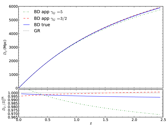
Figure 1: The redshift - comoving distance relation for the $\Lambda$CDM model (black dotted line), the BD model with $\zeta=0.01$ (blue solid line) and the apparent comoving distance for $\gamma_{G}=3/2$ (red dashed line) and $\gamma_{G}=5$ (green dash-dotted line).

First let us consider the effect of the BD model on the comoving distance. In Figure 1, we plot the comoving distance for the $\Lambda$CDM model, the (true) comoving distance for the BD model with $\zeta=0.01$, and the apparent comoving distance for $\gamma_{G}=3/2$ and $\gamma_{G}=5$, as well as the relative difference with respect to the GR model. As we can see, there are some differences in the redshift-distance relation between the GR model and the BD model. If we know how the SNIa luminosity is affected by the variation of $G$ and take this into account as in Equation (11), using the SNIa data we would have obtained the true comoving distance just as those derived from the BAO data. However, if this variation in SNIa luminosity is not taken into account, we would then get the apparent comoving distance, and it deviates more significantly from the GR redshift-distance relation. Also, as we shall see below, the correction term $\frac{5}{2}\gamma_{G}\log\phi$ requires a large $\gamma_{G}$ to have a significant effect, due to the fact that in BD theory $\phi$ is usually within the range $1\pm 10^{-3}$. Here in the global fit we choose the prior to be $\gamma_{G}\in(-90,+90)$.

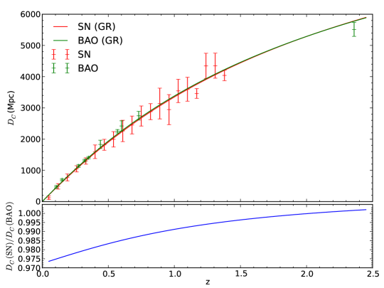
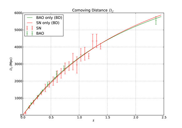
Figure 2: Top: Comoving distances of two flat $\Lambda$CDM models fitted with the SN and BAO data. Bottom: Percent-level discrepancy in comoving distances for the two models.

Figure 3: Fitting the BD model with SNIe data and BAO data separately. Red dots with error bars are the SN data grouped into 20 bins. Green dots are BAO data. The red curve is the fitted curve of SNeIa. The green curve is the fitted curve of BAO. The best fit parameters for SNeIa are $(\Omega_{\Lambda}=0.7326,h=0.7174,\gamma_{G}=7.1143,\zeta=0.0027)$. The best fit parameters for BAO are $(\Omega_{\Lambda}=0.6398,h=0.6623,\zeta=0.0096)$.

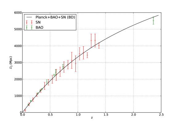
Figure 4: The comoving distances of SN and BAO with a joint constraint of (Planck+BAO+SNIa). The data points representing $D_{C}$ given in this plot have been corrected with the best-fit model.

In Figure 3 we plot the fitting to the GR ($\Lambda$CDM) model with the current SNIa data and BAO data sets. This curve shows that there is a small (percent-level) difference between the best fit of the two data sets, with the BAO data giving slightly larger distances. While it is quite probable that this difference is simply due to statistical fluctuation, the luminosity difference induced by varying $G$ in the SNIa also provides a possible alternative explanation.

In Figure 3, we plot the redshift-comoving distance relation for the best-fit BD model with the BAO data and the (binned) SNIa data separately. We see that although in this case two different data sets are used, the best-fit models give nearly identical $D_{C}(z)$ curves. This is what we would have expected, because in the SN fit the distance measured with BAO is used implicitly, and $\gamma_{G}$ is varied as a free parameter to accommodate the differences between the two.

We then make a joint constraint on the BD model with the Planck+BAO+SNIa data sets, allowing a free $\gamma_{G}$. The result is shown in Figure 4. Here, the SNIa $D^{C}_{L}$ is corrected so that these values can be compared with the BAO data. The redshift distance curve for the joint best-fit model is plotted. We see again that the correction is not large in the end.

These results show that if variation in SNIa luminosity is considered and treated as a free parameter, small differences between the distances measured with separate BAO and SNIa data sets can be reconciled. At present, however, this difference is fairly small, and GR works fine, so one can then constrain the BD model instead.

3.2 Model and Parameter Constraints

In the above, we showed the redshift-distance relation for the best-fit models with various given conditions, in order to illustrate our discussion on effect of SNIa luminosity evolution due to the change of $G$. Here we show how these global fittings were done, and constraints on the BD parameter and other cosmological parameters were obtained with cosmological observational data. To derive such constraints on the BD model, we use the publicly available COSMOMC code (Lewis & Bridle 2002) which implements a Markov-Chain Monte Carlo (MCMC) simulation to explore the parameter space and obtain limits on cosmological parameters. The code was modified earlier by Wu & Chen (2010) to calculate the cosmic evolution with BD gravity. In the current work, we updated the COSMOMC code with newer versions, and also include the new data. Fitting the Planck, BAO and SNIa datasets, we obtain the best fitting results that are summarized in Table 2.

In Figure 6, we plot the 1-D marginalized distribution for the re-parameterized BD model parameter $\zeta$ with different combinations of data sets. The curve which is labeled “Planck” is the result of only using the Planck CMB temperature data. This distribution is relatively broad, as degeneracy of parameters limited the precision of this test. The curve which is labeled “Planck+BAO” plots a combination of the CMB data and the BAO observational data mentioned in Section 2.1, which yields a much tighter constraint. The “Planck+BAO+SN” shows the result combining the Planck, BAO and updated Union2.1 SNIa data together, which is even tighter than the Planck+BAO case, though not by much. Interestingly, the peak of the distribution deviates from the one for the Planck+BAO case, indicating that the SNe could significantly change the result. In the plot, the peaks of the probability distributions are all at $\zeta>0$, slightly favoring the model with $\omega>0$, and especially so when the SNIa data are included in the fit. However, the GR case ($\zeta=0$) is still within the limit, so the fittings are consistent with GR.

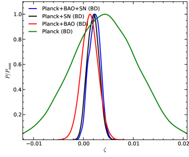
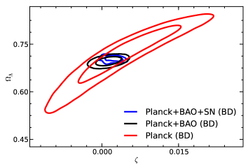
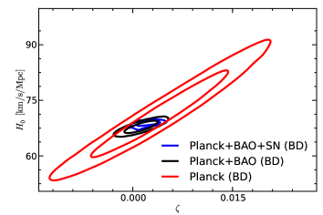
Figure 5: The one dimensional likelihood distribution for $\zeta$. “Planck” denotes the result of only using Planck temperature data. “Planck+BAO” denotes the combined constraint with BAO data mentioned in Sect. 2.1. “Planck+BAO+SN” represents the result after adding the updated Union2.1 SNIa data described in Sect. 2.2.

Figure 6: Left: The two dimensional contours for $\zeta$ versus $\Omega_{\Lambda}$. Right: The two dimensional contour for $\zeta$ versus $H_{0}$.

Figure 6 shows the two dimensional contours for $\zeta$ versus $\Omega_{\Lambda}$ and $H_{0}$. In both cases, we can see that if only the CMB data from Planck are used, there is significant degeneracy as the contours extend to a long “banana” shape. With the addition of the BAO and SNIa data, the degeneracy in the parameters is broken, resulting in much stronger constraints on these parameters.

For the case of the three combined data sets (Planck+BAO+SN), we find the 68% and 95% intervals are

$$0.08\times 10^{-2} <\zeta< 0.33\times 10^{-2}~{}~{}(68\%)\ ;$$ (18)

$$-0.01\times 10^{-2} <\zeta< 0.43\times 10^{-2}~{}~{}(95\%)\ .$$ (19)

These correspond to

$$1249.50>\omega>302.53~{}~{}(68\%)\ ;$$ (20)

$$(\omega<-9999.50)\cup(\omega>232.06)~{}~{}(95\%)\ .$$ (21)

Comparing this with what we obtained using the Planck+BAO data,

$$-0.04\times 10^{-2} <\zeta< 0.28\times 10^{-2}~{}~{}(68\%)\ ;$$ (22)

$$-0.19\times 10^{-2} <\zeta< 0.44\times 10^{-2}~{}~{}(95\%)\ {,}$$ (23)

which correspond to

$$(\omega<-2499.50) ~{}\cup~{} (\omega>356.64)~{}~{}(68\%)\ ;$$ (24)

$$(\omega<-525.82) ~{}\cup~{} (\omega>226.77)~{}~{}(95\%)\ ,$$ (25)

the result is slightly improved.

We can also derive limits on the variation of the gravitational constant using this data set. Note that such limits are somewhat model-dependent, nevertheless they could give an idea about current precision. To do this, we outputted two derived parameters from the MCMC code, i.e. $\dot{G}/G\equiv-\dot{\varphi}/\varphi$, which is the rate of change of the gravitational constant at present, and $\delta G/G\equiv(G_{rec}-G_{0})/G_{0}$, which is the integrated change in the gravitational constant since the epoch of recombination. For the Planck+BAO+SN case, we obtain

$$\dot{G}/G=-0.2649\times 10^{-12},\qquad\delta{G}/G=0.0189$$

and the $68\%$ marginalized limits are

$$-0.3616\times 10^{-12}< \dot{G}/G <-0.0820\times 10^{-12}$$ (26)

$$0.0060< \delta G/G <0.0258\,.$$ (27)

Table 1: Constraints on $\dot{G}/G$. The Errors are $1\sigma$ Unless Otherwise Noted

$\dot{G}/G~{}[10^{-13}$yr${}^{-1}]$	Method
$2\pm 7$	lunar laser ranging (Müller & Biskupek 2007)
$0\pm 4$	Big Bang nucleosynthesis (Copi et al. 2004; Bambi et al. 2005)
$0\pm 16$	helioseismology (Guenther et al. 1998)
$-6\pm 20$	neutron star mass (Thorsett 1996)
$20\pm 40$	Viking lander ranging (Hellings et al. 1983)
$40\pm 50$	binary pulsar (Kaspi et al. 1994)
$-96\sim 81~{}(2\sigma)$	CMB (WMAP3) (Chan & Chu 2007)
$-17.5\sim 10.5~{}(2\sigma)$	WMAP5+SDSS LRG (Wu & Chen 2010)
$-1.42^{+2.48}_{-2.27}~{}(1\sigma)$	Planck+WP+BAO (Li et al. 2013)
$-2.65^{+1.83}_{-0.97}~{}(1\sigma)$	Planck+BAO+SN (This paper)

An updated summary of the various constraints on $\dot{G}/G$ with different methods is given in Table 1. We see that compared with the other method, including high precision solar system experiments, the cosmological constraint we obtain is quite competitive.

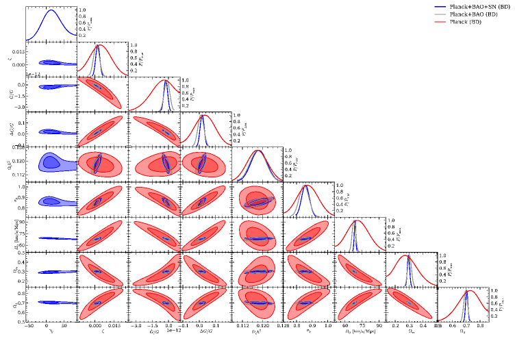
Figure 7: The contours of the marginalized distribution for the parameters in the BD theory.

Table 2: Fit and Limits on Cosmological Model Parameters Obtained with the BD Model

	Planck+BAO+SN (BD)		Planck+BAO (BD)		Planck (BD)
Parameter	Best fit	$68\%$, $95\%$ limits	Best fit	$68\%$, $95\%$ limits	Best fit	$68\%$, $95\%$ limits
$\gamma_{G}$	$67.7232$	$10.5205_{-8.6986-73.7611}^{+42.6913+73.2123}$
$\zeta$	$0.0005$	$0.0024_{-0.0016-0.0025}^{+0.0009+0.0019}$	$0.0017$	$0.0013_{-0.0017-0.0032}^{+0.0015+0.0031}$	$0.0040$	$0.0043_{-0.0068-0.0129}^{+0.0065+0.0128}$
$\Omega_{\mathrm{c}}h^{2}$	$0.1172$	$0.1183_{-0.0022-0.0042}^{+0.0022+0.0044}$	$0.1184$	$0.1181_{-0.0021-0.0042}^{+0.0024+0.0046}$	$0.1187$	$0.1179_{-0.0027-0.0053}^{+0.0027+0.0054}$
$\sigma_{8}$	$0.8474$	$0.8560_{-0.0191-0.0350}^{+0.0177+0.0353}$	$0.8605$	$0.8479_{-0.0201-0.0395}^{+0.0216+0.0422}$	$0.8648$	$0.8695_{-0.0515-0.1001}^{+0.0535+0.1048}$
$\Omega_{\mathrm{b}}h^{2}$	$0.0216$	$0.0215_{-0.0002-0.0005}^{+0.0003+0.0005}$	$0.0217$	$0.0215_{-0.0002-0.0005}^{+0.0002+0.0005}$	$0.0215$	$0.0215_{-0.0003-0.0006}^{+0.0003+0.0006}$
$H_{0}$ 1	$67.7563$	$68.9783_{-0.9628-1.5877}^{+0.2284+0.6046}$	$68.3716$	$67.7557_{-0.9612-1.9476}^{+1.1600+2.2038}$	$70.4907$	$71.2350_{-7.4578-13.8141}^{+7.5226+15.3996}$
$\Omega_{\mathrm{m}}$	$0.3023$	$0.2956_{-0.0050-0.0106}^{+0.0073+0.0140}$	$0.2997$	$0.3038_{-0.0093-0.0177}^{+0.0089+0.0181}$	$0.2821$	$0.2601_{-0.0371-0.0775}^{+0.0856+0.1695}$
$\Omega_{\Lambda}$	$0.6977$	$0.7044_{-0.0073-0.0140}^{+0.0050+0.0106}$	$0.7003$	$0.6962_{-0.0089-0.0181}^{+0.0093+0.0177}$	$0.7179$	$0.7399_{-0.0856-0.1695}^{+0.0371+0.0775}$

Notes: ¹ $H_{0}$ is in units of [km s^-1 Mpc^-1].

We also obtained the best-fit and limits on various cosmological parameters by using the BD model with combinations of data sets that included Planck only, Planck+BAO and Planck+BAO+SN. These results are given in Table 2. We have already discussed the constraint provided by the parameter $\zeta$ or equivalently $\omega$. For other parameters, the precisions of the constraints are generally comparable with the GR case. The contour plots for the model parameters are shown in Figure 7. These plots show that with the addition of the BAO and SNIa data, the constraints on the parameter space could be greatly tightened.

In summary, we have updated the cosmological constraints related to the BD theory with new observational data including the Planck observation of CMB, BAO observation by SDSS and WiggleZ, and also the SNIa observations using the Union2.1 sample. We added the SNIa observations to the data set used in this work, and also considered how variation of $G$ may affect the SNIa peak luminosity. We find the result is still consistent with GR within error limits. We derived limits on $\zeta$ (or equivalently $\omega$) and $\dot{G}$. For the combined fits, the limits are significantly reduced.