Towards composition of conformant systems

Abstract

Motivated by the Model-Based Design process for Cyber-Physical Systems, we consider issues in conformance testing of systems. Conformance is a quantitative notion of similarity between the output trajectories of systems, which considers both temporal and spatial aspects of the outputs. Previous work developed algorithms for computing the conformance degree between two systems, and demonstrated how formal verification results for one system can be re-used for a system that is conformant to it. In this paper, we study the relation between conformance and a generalized approximate simulation relation for the class of Open Metric Transition Systems (OMTS). This allows us to prove a small-gain theorem for OMTS, which gives sufficient conditions under which the feedback interconnection of systems respects the conformance relation, thus allowing the building of more complex systems from conformant components.

I Introduction

In Model-Based Design (MBD) of systems, an executable model of the system is developed early in the design process. This allows the verification engineers to conduct early testing [3]. The model is then refined iteratively and more details are added, e.g., initially ignored physical phenomena, time delays, etc. This eventually leads to the final model that gets implemented on some computational platform, for example via automatic code generation. See Fig. 1.

Each of the above transformations and calibrations introduces discrepancies between the output behavior of the original system (the nominal system) and the output behavior of the derived system (the derived system). These discrepancies are spatial (e.g., slightly different signal values in response to same stimulus, dropped samples, etc) and temporal (e.g., different timing characteristics of the outputs, out-of-order samples, delayed responses, etc) and their magnitude can vary as time progresses.

Ideally, the initial (simpler) model should be amenable to formal synthesis and verification methods (cycle 1 in Fig. 1) through tools like [5, 18]. To understand how the formal verification results on the simpler nominal model can be applied to the derived more complex system, it is necessary to quantify the conformance degree between them. The conformance degree, introduced in [1, 2], is a measure of both spatial and temporal differences between the output behaviors of two systems. It relaxes traditional notions of distance, like sup norm and approximate simulation, to encompass a larger class of systems, and to allow re-ordering of output signal values. In [2], it was shown how the formal properties satisfied by the derived system can be automatically obtained from knowledge of the properties satisfied by the nominal system, and knowledge of the conformance degree between them.

Figure 1: Model-Based Development V-process.

In this paper, we extend that work by studying feedback interconnections of systems. Specifically, we are concerned with the following question: suppose we have a feedback interconnection of a plant and controller, and the closed-loop system has been formally verified to satisfy some properties. If the controller (or the plant) is replaced by another controller which is conformant to it, is the new closed-loop system conformant to the original closed-loop system? If yes, can we estimate its conformance degree without explicitly re-computing it? A positive answer to both questions would allow us to leverage the results in [2] and automatically deduce the properties satisfied by the new interconnection.

In this paper, we give a positive answer to both questions for a general class of dynamical systems modeled as Open Metric Transition Systems (OMTS). These are defined in Section II-A. The tool we use is a generalized notion of Space-Time Approximate Simulation (STAS) relation, which is defined in Section III-A. We show in Section III-B that the existence of such a relation between two OMTS implies that they are also conformant, and yields the conformance degree between them. In Section IV we provide a small-gain theorem for OMTS, which gives sufficient conditions under which feedback interconnections of OMTS respect approximate simulation, and therefore conformance. This is done via STAS functions, which are Lyapunov-like functions that certify the existence of a STAS relation between two systems.

Notation. For a positive integer $n$, $[n]=\{1,\ldots,n\}$. Given a set $\Sigma$, $\Sigma^{*}$ is the set of finite strings on $\Sigma$, i.e. $\Sigma^{*}=\{s_{0}s_{1}\ldots s_{n}\;|\;s_{i}\in\Sigma,n\in\mathbb{N}\}$. Given two sets $A,B$ and $(a,b)\in A\times B$, ${\bf pr}_{A}((a,b))=a$.

II Conformance of Open Metric Transition Systems

In this section, we define a general system model, namely, Open Metric Transition Systems (OMTS). These extend Metric Transition Systems [8] in that they allow interconnection of systems, and will be our formalism of choice in this paper. We then define the conformance relations for OMTS and feedback interconnections for OMTS, which allows us to speak of controlled OMTS and compositionality in Section IV. As an illustration, we show how hybrid systems can be modeled as OMTS.

II-A Open metric transition systems and conformance

A Metric Transition System (MTS) serves to model, at an abstract level, a fairly large class of systems. An MTS is a tuple $T=(Q,\Sigma_{\chi},\rightarrow,Q^{0},\Pi,\left\langle\;\right\rangle)$ where $Q$ is a set known as the state space, $Q^{0}\subset Q$ is the set of initial states, $\Sigma_{\chi}$ is the set of labels on which transitions take place, $\xrightarrow{\;}\subset Q\times\Sigma_{\chi}\times Q$ is the transition relation, $\Pi$ is the output set, and $\left\langle\right\rangle:Q\rightarrow\Pi$ is the output map. We write $q\xrightarrow{\sigma_{\chi}}q^{\prime}$ to denote an element $(q,\sigma_{\chi},q^{\prime})\in\rightarrow$. Both $Q$ and $\Pi$ are metric spaces, that is, they are equipped with metrics $d_{Q}$ and $d_{\Pi}$. Moreover, for any $q\in Q$ and any label subset $S\subset\Sigma_{\chi}$, the set

$$\text{Post}(q,S)=\cup_{\sigma_{\chi}\in S}\text{Post}(q,\sigma_{\chi})$$ (1)

is compact in the metric-induced topology.

Given a string of labels $\bar{\sigma_{\chi}}={\sigma_{\chi}}_{,1}{\sigma_{\chi}}_{,2}\ldots{\sigma_{\chi}}_{,m}$, we write ${\bar{\sigma_{\chi}}}_{[i]}\in\Sigma_{\chi}^{*}$ for the prefix string ${\sigma_{\chi}}_{,1}{\sigma_{\chi}}_{,2}\ldots{\sigma_{\chi}}_{,i}$, $i\leq m$. The sets $\Sigma_{\chi}$ and $\Sigma_{\chi}^{*}$ are equipped with pseudo-metrics $d_{\Sigma_{\chi}}$ and $d_{\Sigma_{\chi}^{*}}$, respectively, and $\Pi$ is equipped with a metric $d_{\Pi}$. When two MTS share the same $\Sigma_{\chi}$ ($\Sigma_{\chi}^{*}$, $\Pi$), they also share the same associated (pseudo-)metrics.

An Open Metric Transition System (OMTS) is a tuple $T=(Q,\Sigma,\xrightarrow{}_{T},Q^{0},\Pi,\left\langle\;\right\rangle,p)$ where $(Q,\Sigma,\rightarrow_{T},Q^{0},\Pi,\left\langle\;\right\rangle)$ is an MTS as above. The label set $\Sigma$ of an OMTS has a special structure: $\Sigma\subset\Sigma_{u}\times\Sigma_{\chi}$ for sets $\Sigma_{u},\Sigma_{\chi}$. The intuition behind this division is that $\Sigma_{u}$ will be used to model input signals to the system embedded as an OMTS, and $\Sigma_{\chi}$ will be used to model the domain of that input signal. This departs from earlier approaches to embedding forced dynamical systems as MTS [7], because we need a way to describe interconnections of MTS, while preserving timing information in the interconnection. A generic label $\sigma$ thus has two components: $\sigma=(\sigma_{u},\sigma_{\chi})$. The string prefix $\bar{\sigma}_{[i]}$ is defined similarly to the case of MTS. The port map $p:(\xrightarrow{}_{T})\rightarrow\Sigma\cup\{\nu\}$ associates a label to each transition in $\xrightarrow{}_{T}$, or a special empty label $\nu$. The empty label, as we will see, is used to allow a system to make empty transitions which don’t change its state and don’t advance time. The output of the port map will be used to compose OMTS. This makes them similar to hybrid I/O automata [14] but enriched with a metric structure, and with ‘discrete actions’ and ‘trajectories of input variables’ lumped into one label set, which fits well our usage of hybrid time.

We now define conformance between two OMTS $T_{1}$ and $T_{2}$. Conformance quantifies the similarity between systems, and accounts for the fact that in a typical MBD process (Fig. 1), the output signals of the derived model will have temporal and spatial differences with the outputs of the nominal model. From the knowledge of the conformance degree between two systems, we can conclude what formal specifications are satisfied by one, given the specifications satisfied by the other [2].

Definition II.1 (Conformance)

Let $T_{1}$ and $T_{2}$ be two OMTS with a common output space $\Pi$ and common label set $\Sigma$. Let $\tau,\varepsilon$ be two non-negative reals. Let $D\subset Q_{1}^{0}\times Q_{2}^{0}$ be a relation defined on their initial sets. We refer to $D$ as the derivation relation. We say $T_{2}$ conforms to $T_{1}$ with precision $\mathbf{(\tau,\varepsilon)}$ and derivation relation $D$, which we write $T_{1}\preceq^{C}_{\tau,\varepsilon}T_{2}$, if for all $(q_{1}^{0},q_{2}^{0})\in D$, and any sequence of $T_{1}$ transitions

$$q_{1}^{0}\xrightarrow{\sigma_{1}}_{1}q_{1}^{1}\xrightarrow{\sigma_{2}}_{1}q_{1}^{2}\xrightarrow{...}_{1}\ldots\xrightarrow{\sigma_{n}}_{1}q_{1}^{m}$$

there exists a sequence of $T_{2}$ transitions

$$q_{2}^{0}\xrightarrow{\alpha_{1}}_{2}q_{2}^{1}\xrightarrow{\alpha_{2}}_{2}q_{2}^{2}\xrightarrow{...}_{2}\ldots\xrightarrow{\alpha_{n}}_{2}q_{2}^{m^{\prime}}$$

such that

1. for all $q_{1}^{i}$, $i\in[m]$, there exists $q_{2}^{k}$ s.t. $d_{\Pi}(\left\langle q_{1}^{i}\right\rangle,\left\langle q_{2}^{k}\right\rangle)\leq\varepsilon$ and $d_{\Sigma^{*}}(\bar{\sigma}_{[i]},\bar{\alpha}_{[k]})\leq\tau$

2. for all $q_{2}^{i}$, $i\in[m^{\prime}]$, there exists $q_{1}^{k}$ s.t. $d_{\Pi}(\left\langle q_{1}^{k}\right\rangle,\left\langle q_{2}^{i}\right\rangle)\leq\varepsilon$ and $d_{\Sigma^{*}}(\bar{\sigma}_{[k]},\bar{\alpha}_{[i]})\leq\tau$

Intuitively, the definition requires $T_{2}$ to be able to match any execution of $T_{1}$, with some allowed deviation between the states that each execution visits, and some allowed deviation between the labels on which transitions take place. The matching is required not only for the final reached states $q_{1}^{m}$ and $q_{2}^{m^{\prime}}$, but for all intermediary states. The relation $D$ is meant to capture the mapping between the initial states of one model ($T_{1}$) and the initial states of its implementation ($T_{2}$). For example, if $T_{2}$ is obtained by model order reduction from $T_{1}$, $D$ captures the reduction mapping as applied to the initial states. Because some of the labels in either transition sequence may be the empty label $\nu$, more than one state in one sequence may match with the same state in the other sequence.

II-B Feedback interconnection of OMTS

Given two OMTS $T_{1}$ and $T_{2}$, we define their feedback interconnection as follows.

Definition II.2 (Feedback in OMTS)

Let $T_{i}$ be an OMTS $(Q_{i},\Sigma,\xrightarrow{\;}_{i},Q_{i}^{0},\Pi_{i},\left\langle\;\right\rangle_{i},p_{i})$, $i=1,2$, such that $\Sigma=\Sigma_{u}\times\Sigma_{\chi}$. Assume that $\Sigma\supset p_{2}(\xrightarrow{\;}_{2})$ and $\Sigma\supset p_{1}(\xrightarrow{\;}_{1})$. Their feedback interconnection is a (closed) MTS $(Q,{\Sigma_{\chi}}_{12},\xrightarrow{\;},Q^{0},\Pi,\left\langle\;\right\rangle)$, denoted $T_{1}\circ T_{2}$, where

• $Q=Q_{1}\times Q_{2}$

• ${\Sigma_{\chi}}_{12}\subset\Sigma_{\chi}$

• $Q^{0}=Q_{1}^{0}\times Q_{2}^{0}$

• $\Pi=\Pi_{1}\times\Pi_{2}$

• $\left\langle(q_{1},q_{2})\right\rangle=(\left\langle q_{1}\right\rangle_{1},\left\langle q_{2}\right\rangle_{2})$

• $\xrightarrow{}$: $(q_{1},q_{2})\xrightarrow{\sigma_{\chi}}(q_{1}^{\prime},q_{2}^{\prime})$ iff $\exists\sigma_{1}=(\sigma_{1,u},\sigma_{\chi})\in\Sigma$ and $\sigma_{2}=(\sigma_{2,u},\sigma_{\chi})\in\Sigma$ s.t. $q_{1}\xrightarrow{\sigma_{1}}_{1}q_{1}^{\prime}$, $q_{2}\xrightarrow{\sigma_{2}}_{2}q_{2}^{\prime}$, and $\sigma_{1}=p_{2}(q_{2}\xrightarrow{\sigma_{2}}_{2}q_{2}^{\prime})$, $\sigma_{2}=p_{1}(q_{1}\xrightarrow{\sigma_{1}}_{1}q_{1}^{\prime})$.

The output set distance is given by

$$d_{\Pi}((q_{1},q_{2}),(q_{1}^{\prime},q_{2}^{\prime}))=\tilde{h}(d_{\Pi_{1}}(q_{1},q_{1}^{\prime}),d_{\Pi_{2}}(q_{2},q_{2}^{\prime}))$$

for some positive non-decreasing function $\tilde{h}$.

This is meant to model the situation when two hybrid systems are feedback interconnected, such that $T_{1}$’s outputs constitute the inputs to $T_{2}$, and vice versa. Note that the definitions of output set, output map and associated distance function are somewhat arbitrary and ultimately depend on the application domain.

To simplify the statement of the main theorem and its proof, we introduce the following ‘lifting’ of ${\Sigma_{\chi}}_{12}$ to $\Sigma\times\Sigma$. The set $\Sigma_{12}$ defined below contains all label pairs $(\sigma_{1},\sigma_{2})\in\Sigma_{1}\times\Sigma_{2}$ allowed by the interconnection $T_{1}\circ T_{2}$. Formally:

$$\begin{split}\Sigma_{12}:=\{&(\sigma_{1},\sigma_{2})\in\Sigma\times\Sigma\;|\;\sigma_{1}=p_{2}(q_{2}\xrightarrow{\sigma_{2}}_{2}q_{2}^{\prime}),\\ &\sigma_{2}=p_{1}(q_{1}\xrightarrow{\sigma_{1}}_{1}q_{1}^{\prime}),{\sigma_{\chi}}_{1}={\sigma_{\chi}}_{2}\in{\Sigma_{\chi}}_{12},\\ &\text{ for some transitions }q_{2}\xrightarrow{\sigma_{2}}_{2}q_{2}^{\prime}\text{ and }q_{1}\xrightarrow{\sigma_{1}}_{1}q_{1}^{\prime}\}\end{split}$$ (2)

We note two properties of $\Sigma_{12}$:

1. $\Sigma_{12}\subset\Sigma\times\Sigma$

2. minimizing a function over the transitions enabled by labels in ${\Sigma_{\chi}}_{12}$ yields the same result as minimizing it over the transitions enabled by labels in the lifting $\Sigma_{12}$.

II-C Problem formulation

The formal statement of this paper’s problem follows:

Given two OMTS $T_{1}$ and $T_{2}$ connected in a feedback loop, and OMTS $T_{3}$ that conforms to $T_{1}$ with precision $\mathbf{(\tau,\varepsilon)}$ and derivation relation $D$, is $T_{3}\circ T_{2}$ conformant to the $T_{1}\circ T2$? If yes, what is the conformance degree between the two loops?

II-D Embedding a hybrid system as an OMTS

Hybrid systems can be represented using, or embedded as, OMTS. This enables us to apply the compositionality result to them. We briefly define hybrid systems to show the embedding. Let $C$ and $D$ be subsets of $\mathbb{R}^{n+m}$, $U\subset\mathbb{R}^{m}$ be a set of input values, $F:\mathbb{R}^{n+m}\rightrightarrows\mathbb{R}^{n}$ and $G:\mathbb{R}^{n+m}\rightrightarrows\mathbb{R}^{n}$ be set-valued maps with $C\subset\mathbf{dom}F$ and $D\subset\mathbf{dom}G$. Let $z:\mathbb{R}^{n}\rightarrow\mathbb{R}^{n_{z}}$ be a function. The hybrid dynamical system $\mathcal{H}$ with data $(C,F,D,G,z)$, internal state $x\in\mathbb{R}^{n}$ and output $y\in\mathbb{R}^{n_{z}}$ is governed by [10]

$$\mathcal{H}\left\{\begin{array}[]{lll}\dot{x}&\in F(x,u)&\quad(x,u)\in C\\ x^{+}&\in G(x,u)&\quad(x,u)\in D\\ y&=z(x)\end{array}\right.$$ (3)

The ‘jump’ map $G$ models the change in system state at a mode change, or ‘jump’, and the jump set $D$ captures the conditions causing a jump. The ‘flow’ map $F$ models state evolution away from jumps, while $(x,u)$ is in the flow set $C$. System trajectories start from a specified set of initial conditions $H_{0}\subset{\bf pr}_{\mathbb{R}^{n}}(\overline{C}\cup D)$. Finally, the output of the system $y$ is given as a function $z$ of its internal state, and its input is given by $u$ which takes values in a set $U$.

Solutions $(\mathbf{\phi},\mathfrak{u}$) to (3) are given by a hybrid arc $\mathbf{\phi}$ and an input arc $\mathfrak{u}$ sharing the same hybrid time domain $\mathbf{dom}\mathbf{\phi}=\mathbf{dom}\mathfrak{u}$, and with standard properties that can be reviewed in [9, Ch. 2] .

Definition II.3 (Hybrid time domains and arcs [10])

A subset $E\subset\mathbb{R}_{+}\times\mathbb{N}$ is a compact hybrid time domain if

$$E=\bigcup_{j=0}^{J-1}[t_{j},t_{j+1}]\times\{j\}$$

for some finite increasing sequence of times $0=t_{0}\leq t_{1}\leq t_{2}\leq\ldots\leq t_{J}$. A hybrid arc $\mathbf{\phi}$ is a function supported over a hybrid time domain $\mathbf{\phi}:E\rightarrow\mathbb{R}^{n}$, such that for every $j$, $\mathbf{\phi}(\cdot,j)$ is locally absolutely continuous in $t$ over $I_{j}=\{t:(t,j)\in E\}$; we call $E$ the domain of $\mathbf{\phi}$ and write it $\mathbf{dom}\mathbf{\phi}$.

A hybrid system $\mathcal{H}=(C,F,D,G,z)$ can be embedded as an OMTS $T=(Q,\Sigma,\rightarrow,Q^{0},\Pi,\left\langle\;\right\rangle,p)$ as follows: $Q=\{x\in\mathbb{R}^{n}\;|\;\exists u:(x,u)\in\overline{C}\cup D\}$, $Q^{0}\subset Q$, $\left\langle\;\right\rangle=z$, and $\Pi=\mathbb{R}^{n_{z}}$. The label set is made of input arcs and their domains, and the empty label $\nu$:

$$\Sigma=\{(\mathfrak{u},\mathbf{dom}\mathfrak{u})\;|\;\mathfrak{u}\text{ is an input arc}\}\cup\{\nu\}$$ (4)

The transition relation is defined as $q\xrightarrow{\sigma}q^{\prime}$ iff either $\sigma=\nu$ is the empty label and $q=q^{\prime}$, or $\sigma=(\mathfrak{u},\mathbf{dom}\mathfrak{u})$ and there exists a solution pair $(\mathbf{\phi},\mathfrak{u})$ s.t. $\mathbf{\phi}(0,0)=q,\mathbf{\phi}(t,j)=q^{\prime}$ for some $(t,j)$ in $\mathbf{dom}\mathfrak{u}$. The port map $p$ is defined as

$$p(q\xrightarrow{\sigma}q^{\prime})=\left\{\begin{matrix}(z(q),(0,0))&if\sigma=\nu\\ (z\circ\mathbf{\phi},\mathbf{dom}\mathbf{\phi})&\text{ otherwise}\end{matrix}\right.$$

where $(\mathbf{\phi},\mathfrak{u})$ is the solution pair of $\mathcal{H}$ corresponding to $\sigma$ as defined above in (4).

Later in the paper, we will need to impose a requirement on $d_{\Sigma}$, namely, equation (5) from Section III-B. The rest of this section shows how $d_{\Sigma}$ can be defined so this requirement is met. First, given an input arc $\mathfrak{u}$ with domain $E$ and two subsets $E^{\prime}\subset E$, $E^{\prime\prime}\subset E$ such that $(0,0)\in E^{\prime}\cap E^{\prime\prime}$ and $\sup_{j}E^{\prime}=\sup_{j}E^{\prime\prime}$, the restrictions of $\mathfrak{u}$ to $E^{\prime}$ and $E^{\prime\prime}$ respectively are said to have a common extension. (So the restricted arcs start at $(0,0)$ and make the same number of jumps).

Let $\sigma=(\mathfrak{u},E),\sigma^{\prime}=(\mathfrak{u}^{\prime},E^{\prime})$ be two labels with $E=\cup_{j}^{J-1}I_{j}\times\{j\}$, $E^{\prime}=\cup_{j}^{J^{\prime}-1}I^{\prime}_{j}\times\{j\}$ compact hybrid time domains with $J$ and $J^{\prime}$ jumps, respectively. Define

$$d_{\Sigma}(\sigma,\sigma^{\prime}):=\left\{\begin{matrix}\max_{j}d_{H}(I_{j},I_{j}^{\prime})&&\text{$\mathfrak{u}$ and $\mathfrak{u}^{\prime}$ have a}\\ \;&&\text{common extension}\\ \infty&&\text{ otherwise }\end{matrix}\right.$$

Here, $d_{H}$ is the symmetric Haussdorff distance between two sets. A string $s=\sigma_{1}\sigma_{2}\ldots\sigma_{m}$ is then a concatenation of the input arcs and their hybrid time domains , and is itself a valid pair (input arc, hybrid time domain). That is, in this case, $\Sigma^{*}\subset\Sigma$. Therefore given two strings $s$ and $a$, we simply define $d_{\Sigma^{*}}(s,a)=d_{\Sigma}(s,a)$. It can be shown that this satisfies (5).

III From simulation relations to conformance relations

III-A Space-Time Approximate Simulations

A Space-Time Approximate Simulation (STAS) relation is an approximate simulation relation in the sense of [12]. We choose to introduce the new terminology in order to avoid potentially awkward (and possibly confusing) references to ‘simulation relations in the sense of [xyz]’. STAS were introduced in [12] and applied in [13] to the study of networked control systems.

Our interest in this paper is on conformance as defined earlier, which is a notion defined on entire trajectories. STAS relations, defined on individual states of systems, is a related notion which has the advantage of having a functional characterization, much like Lyapunov functions characterize stability. In this section, we define STAS relations and connect them to conformance. The functional characterization of STAS can then be used to characterize conformance.

Definition III.1 (STAS)

Given two OMTS $T_{i}=(Q_{i},\Sigma,\xrightarrow{}_{i},Q_{i}^{0},\Pi,\left\langle\right\rangle_{i},p_{i}),i=1,2$, and positive reals $\tau,\varepsilon$, consider a relation $R\subset Q_{1}\times Q_{2}$, and the following three conditions:

1. $\forall(q_{1},q_{2})\in R$, $d_{\Pi}(\left\langle q_{1}\right\rangle,\left\langle q_{2}\right\rangle)\leq\varepsilon$

2. $\forall(q_{1},q_{2})\in R$, $\forall q_{1}\xrightarrow{\sigma_{1}\in\Sigma}q_{1}^{\prime}$, $\exists\sigma_{2}\in B_{\tau}(\sigma_{1})$ and a transition $q_{2}\xrightarrow{\sigma_{2}}q_{2}^{\prime}$ s.t. $(q_{1}^{\prime},q_{2}^{\prime})\in R$

3. $\forall q_{1}^{0}\in Q_{1}^{0},\exists q_{2}^{0}\in Q_{2}^{0}$ s.t. $(q_{1}^{0},q_{2}^{0})\in R$

where $B_{\tau}(\sigma)=\{\sigma^{\prime}\in\Sigma\;|\;d_{\Sigma}(\sigma,\sigma^{\prime})\leq\tau\}$. If $R$ satisfies the first 2 conditions, then it is a $\mathbf{(\tau,\varepsilon)}$-space-time approximate simulation (STAS) of $T_{1}$ by $T_{2}$. If in addition it satisfies the third, then we say $T_{2}$ simulates $T_{1}$ with precision $(\tau,\varepsilon)$.

STAS relations describe what happens when $T_{1}$ ‘plays’ label $\sigma_{1}$, and $T_{2}$ is allowed to respond by playing a label from $B_{\tau}(\sigma_{1})$. In particular, it says that $T_{2}$ can always find a label such that the distance between the reached outputs is less than $\varepsilon$. In the rest of this paper, we will often simply speak of a simulation to mean a STAS.

III-B From simulation to conformance

The connection between STAS, which is a relation between states, and conformance, which is a relation between executions, is captured in the following proposition.

Proposition III.1

Given two OMTS $T_{i}=(Q_{i},\Sigma,\xrightarrow{}_{i},\Pi,\left\langle\right\rangle_{i},g_{i}),i=1,2$, let $R$ be a $(\tau,\varepsilon)$-STAS relation between them, and let $D\subset Q_{1}^{0}\times Q_{2}^{0}$ be a derivation relation between them. Assume that the label pseudo-metrics $d_{\Sigma}$, $d_{\Sigma^{*}}$ are such that for any two strings $\bar{\sigma}=\sigma_{1}\ldots\sigma_{i}$ and $\bar{\alpha}=\alpha_{1}\ldots\alpha_{i}$,

$$(\forall k\leq i,d_{\Sigma}(\sigma_{k},\alpha_{k})\leq\tau)\;\implies d_{\Sigma^{*}}(\bar{\sigma}_{[i]},\bar{\alpha}_{[i]})\leq\tau$$ (5)

If $D\subset R$, then $T_{2}$ conforms to $T_{1}$ with precision $(\tau,\varepsilon)$ and with derivation relation $D$. $\square$

Proof:

Take any pair $(q_{1}^{0},q_{2}^{0})\in D$, and any sequence of $T_{1}$ transitions

$$q_{1}^{0}\xrightarrow{\sigma_{1}}q_{1}^{1}\xrightarrow{\sigma_{2}}q_{1}^{2}\xrightarrow{\sigma_{3}}\ldots\xrightarrow{\sigma_{n}}q_{1}^{n}$$

Because $D\subset R$, there exists a $T_{2}$ transition $q_{2}^{0}\xrightarrow{\alpha_{1}}q_{2}^{1}$ s.t. $\alpha_{1}\in B_{\tau}(\sigma_{1})$ and $(q_{1}^{0},q_{2}^{0})\in R$, therefore $d_{\Pi}(\left\langle q_{1}^{1}\right\rangle,\left\langle q_{2}^{1}\right\rangle)\leq\varepsilon$. Proceeding in this way for every $k\leq n$, we build a sequence $\mathbf{q_{2}}$ of $T_{2}$ transitions

$$\mathbf{q_{2}}=q_{2}^{0}\xrightarrow{\alpha_{1}}q_{2}^{1}\xrightarrow{\alpha_{2}}q_{2}^{2}\xrightarrow{...}\ldots\xrightarrow{\alpha_{n}}q_{2}^{n}$$

such that $d_{\Sigma}(\sigma_{k},\alpha_{k})\leq\tau$ and $d_{\Pi}(\left\langle q_{1}^{k}\right\rangle,\left\langle q_{2}^{k}\right\rangle)\leq\varepsilon$ for all $k$.

Now we check condition (a) of Def.II.1. For any $q_{1}^{i},i\leq n$, $d_{\Pi}(\left\langle q_{1}^{i}\right\rangle,\left\langle q_{2}^{i}\right\rangle)\leq\varepsilon$ and by property (5) of the label pseudo-metric, $d_{\Sigma^{*}}(\sigma_{[i]},\alpha_{[i]})\leq\tau$. Thus condition (a) is satisfied. By construction of the execution $\mathbf{q_{2}}$ and symmetry of $d_{\Pi}$ and $d_{\Sigma}$, we also have condition (b). ∎

IV Compositionality

In this section, we prove a general small gain condition under which the feedback interconnection of OMTS preserves similarity relations. By Prop. III.1, this implies that conformance is also preserved under these conditions. We work in the OMTS formalism as it bypasses unnecessary technicalities and allows us to establish the result in greater generality, while maintaining continuity with the work of [13].

IV-A Compositionality of similar metric transition systems

Consider OMTS $T_{1},T_{2},T_{3},T_{4}$ with label sets $\Sigma_{1}=\Sigma_{2}$ and $\Sigma_{3}=\Sigma_{4}$.

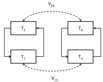
Figure 2: Interconnections of similar MTS

Systems $T_{1}$ and $T_{2}$ are feedback interconnected to yield $T_{1}\circ T_{2}$, with state space $Q_{12}=Q_{1}\times Q_{2}$, and label set ${\Sigma_{\chi}}_{12}$. Similarly, systems $T_{3}$ and $T_{4}$ are feedback interconnected to yield $T_{3}\circ T_{4}$, with state space $Q_{34}=Q_{3}\times Q_{4}$, and label set ${\Sigma_{\chi}}_{34}$. See Fig. 2. We seek conditions under which $T_{3}\circ T_{4}$ simulates $T_{1}\circ T_{2}$; based on Prop.III.1, this would imply that under the same conditions, $T_{1}\circ T_{2}\preceq^{C}_{\tau,\varepsilon}T_{3}\circ T_{4}$ for some $(\tau,\varepsilon)$. To do so, we use the functional characterization of STAS.

Definition IV.1

[12, Def. 3.2] Given two OMTS $T_{1}$ and $T_{2}$ with common output set $\Pi$ and label set $\Sigma$, and non-negative real $\tau$, a function $V:Q_{1}\times Q_{2}\rightarrow\mathbb{R}_{+}\cup\{\infty\}$ is a $\tau$-simulation function of $T_{1}$ by $T_{2}$ if for all $(q_{1},q_{2})\in Q_{1}\times Q_{2}$,

1. $V(q_{1},q_{2})\geq d_{\Pi}(\left\langle q_{1}\right\rangle,\left\langle q_{2}\right\rangle)$

2. $V(q_{1},q_{2})\geq\sup_{q_{1}\xrightarrow{\sigma\in\Sigma}q_{1}^{\prime}}\inf_{q_{2}\xrightarrow{\sigma^{\prime}\in B_{\tau}(\sigma)}q_{2}^{\prime}}V(q_{1}^{\prime},q_{2}^{\prime})$

A $\tau$-simulation function defines a $(\tau,\varepsilon)$-STAS relation via its level sets. Namely, as shown in [12, Thm. 3.4], the $\varepsilon$-sublevel set of $V$

$$\mathcal{L}_{\varepsilon}^{V}=\{(q,q^{\prime})\in Q_{1}\times Q_{2}\;|\;V(q,q^{\prime})\leq\varepsilon\}$$ (6)

is a $(\tau,\varepsilon)$-STAS relation of $T_{1}$ by $T_{2}$ for all $\varepsilon\geq 0$.

To keep the equations readable, in what follows, we define the following: given $\sigma_{12}=(\sigma_{1},\sigma_{2})\in\Sigma_{12}$,

$$B_{\tau}^{34}(\sigma_{12}):=\{(\sigma_{3},\sigma_{4})\in\Sigma_{34}\;|\;d_{\Sigma_{\chi}}({\sigma_{\chi}}_{1},{\sigma_{\chi}}_{3})\leq\tau\}$$

($\Sigma_{34}$ is defined analogously to $\Sigma_{12}$ in (4)). The ball $B_{\tau}^{34}(\sigma_{12})$ contains all labels in $\Sigma_{34}$ whose ‘chronological component’ ${\sigma_{\chi}}_{3}$ is no more than $\tau$-away from ${\sigma_{\chi}}_{1}$. Note that by definition for any $(\sigma_{3},\sigma_{4})\in\Sigma_{34}$, ${\sigma_{\chi}}_{3}={\sigma_{\chi}}_{4}$ (and analogously ${\sigma_{\chi}}_{1}={\sigma_{\chi}}_{2}$) so the above definition effectively bounds the distance between both chronological components of the label.

Consider the OMTS $T_{1},T_{2},T_{3},T_{4}$, with $T_{1}$ in a feedback loop with $T_{2}$, and $T_{3}$ with $T_{4}$. Let $V_{13}$ be a $\tau_{13}$-STAS function of $T_{1}$ by $T_{3}$ (Def. IV.1), and $V_{24}$ be a $\tau_{24}$-STAS function of $T_{2}$ by $T_{4}$. All systems share the same label set $\Sigma$. We introduce the following functions to keep the equations manageable: given $q_{1}^{\prime}\in Q_{1},q_{3}\in Q_{3},\sigma_{i}\in\Sigma$, define

$$\underline{V}_{13}(q_{1}^{\prime},q_{3},\sigma_{1}):=\inf_{q_{3}\xrightarrow{\sigma_{3}\in B_{\tau_{13}}(\sigma_{1})}q_{3}^{\prime}}V_{13}(q_{1}^{\prime},q_{3}^{\prime})$$

$$\underline{V}_{24}(q_{2}^{\prime},q_{4},\sigma_{2}):=\inf_{q_{4}\xrightarrow{\sigma_{4}\in B_{\tau_{24}}(\sigma_{2})}q_{4}^{\prime}}V_{24}(q_{2}^{\prime},q_{4}^{\prime})$$

Consider $\underline{V}_{13}$: if we think of $T_{3}$ as trying to match $T_{1}$ transitions by minimizing $V_{13}$ over the label ball $B_{\tau_{13}}$, then $\underline{V}_{13}$ measures how well it does it. Similarly for $\underline{V}_{24}$.

Because STAS functions certify STAS relations via (6), the following theorem provides a way to build STAS functions for interconnections of systems, from the STAS functions of the individual connected systems.

Theorem IV.1

Consider the OMTS $T_{1},T_{2},T_{3},T_{4}$ with common label set $\Sigma$ interconnected as described above. Let $V_{13}$ be a $\tau_{13}$-STAS function of $T_{1}$ by $T_{3}$, and $V_{24}$ be a $\tau_{24}$-STAS function of $T_{2}$ by $T_{4}$. Set $\tau=\min(\tau_{13},\tau_{24})$.

Define $V:Q_{12}\times Q_{34}\rightarrow\overline{\mathbb{R}_{+}}$ to be $V((q_{1},q_{2}),(q_{3},q_{4}))=h(V_{13}(q_{1},q_{3}),V_{24}(q_{2},q_{4}))$ where $h$ is continuous and non-decreasing in both arguments.

Recall the definition of lifted label sets $\Sigma_{12},\Sigma_{34}$ in (2). Let $g:\mathbb{R}\rightarrow\mathbb{R}$ be a non-decreasing function s.t. $g(x)\geq x$ and for all $q_{12}\in Q_{12}$, $q_{34}\in Q_{34}$, $g$ satisfies

$$\sup_{q_{12}\xrightarrow{(\sigma_{1},\sigma_{2})\in\Sigma\times\Sigma}q_{12}^{\prime}}h(\underline{V}_{13}(q_{1}^{\prime},q_{3},\sigma_{1}),\underline{V}_{24}(q_{2}^{\prime},q_{4},\sigma_{2}))\geq\;$$

$$g\left(\sup_{q_{12}\xrightarrow{(\sigma_{1},\sigma_{2})\in\Sigma_{12}}q_{12}^{\prime}}h(\underline{V}_{13}(q_{1}^{\prime},q_{3},\sigma_{1}),\underline{V}_{24}(q_{2}^{\prime},q_{4},\sigma_{2}))\right)$$

(7)

Also, let $\gamma_{1},\gamma_{2}:\mathbb{R}\rightarrow\mathbb{R}_{+}$ be continuous non-increasing functions s.t. $\gamma_{i}(x)\leq x$, $i=1,2$, and for all $\sigma_{12}=(\sigma_{1},\sigma_{2})\in\Sigma_{12}$, for all $(q_{3},q_{4})\in Q_{34}$, and all $(q_{1}^{\prime},q_{2}^{\prime})\in Q_{12}$

$$\underline{V}_{13}(q_{1}^{\prime},q_{3},\sigma_{1})\geq\gamma_{1}(\inf_{q_{3}\xrightarrow{B_{\tau}^{34}(\sigma_{12})}q_{3}^{\prime}}V_{13}(q_{1}^{\prime},q_{3}^{\prime}))$$ (8)

$$\underline{V}_{24}(q_{2}^{\prime},q_{4},\sigma_{2})\geq\gamma_{2}(\inf_{q_{4}\xrightarrow{B_{\tau}^{34}(\sigma_{12})}q_{4}^{\prime}}V_{24}(q_{2}^{\prime},q_{4}^{\prime}))$$ (9)

If the following conditions hold:

1. $V$ is continuous in the product topology of $Q_{12}\times Q_{34}$.

2. For all $q_{12}\in Q_{1}\times Q_{2},q_{34}\in Q_{3}\times Q_{4}$,

   $$V(q_{12},q_{34})\geq d_{\Pi}(\left\langle q_{12}\right\rangle,\left\langle q_{34}\right\rangle)$$ (10)

3. Function $g$ distributes over $h$, that is

   $$g(h(x,x^{\prime}))=h(g(x),g(x^{\prime}))\;\forall x,x^{\prime}$$

4. [Small Gain Condition] For all $x\in\mathbb{R}$,

   $$g\circ\gamma_{1}(x)\geq x,\;g\circ\gamma_{2}(x)\geq x$$

then $V$ is a $\tau$-STAS function of $T_{1}\circ T_{2}$ by $T_{3}\circ T_{4}$. $\square$

Before proving the theorem, a few words are in order about its hypotheses. A function $g$ satisfying (7) always exists: by observing that $\Sigma_{12}\subset\Sigma\times\Sigma$, we see that $g$ can be taken to be the identity. A non-identity function quantifies how restrictive is the interconnection $T_{1}\circ T_{2}$. It does so by quantifying the difference between the full label set $\Sigma\times\Sigma$ available to the individual systems operating without interconnection (on the LHS of inequality (7)), and the restricted label set $\Sigma_{12}$ available to them as part of the interconnection (on the RHS).

Similarly, functions $\gamma_{1},\gamma_{2}$ satisfying (9) always exist: we can take $\gamma_{i}$ to be identically zero. These choices, however, are unlikely to be useful: we need $\gamma_{i}$ to quantify how restrictive is the interconnection $T_{3}\circ T_{4}$. They do so by quantifying the difference between the full label ball $B_{\tau_{13}}(\sigma_{1})\times B_{\tau_{24}}(\sigma_{2})$ available to the individual systems operating without interconnection, and the restricted label ball $B_{\tau}^{34}(\sigma_{12})\subset B_{\tau_{13}}(\sigma_{1})\times B_{\tau_{24}}(\sigma_{2})$ available to them as part of the interconnection. See Fig.3 for an illustration of the label sets.

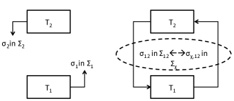
Figure 3: Label sets constrained by interconnection. $\Sigma_{12}$ is the set of label pairs compatible with the interconnection as given in Def.II.2.

These two aspects are similar to the conditions, in more classical Lyapunov-based small gain theorems, placing a minimum on the rate of decrease of the Lyapunov functions of the individual systems, and that bound is related to the growth of the other system’s Lyapunov function. (For example results on input-to-state stability [11],[21], and for bisimulation functions in non-hybrid systems [6]). Now the more restrictive $T_{1}\circ T_{2}$ is, the bigger $g$ can be. The more restrictive $T_{3}\circ T_{4}$ is, the smaller $\gamma_{i}$ need to be. The Small Gain Condition (SGC) says that the restrictiveness of $T_{1}\circ T_{2}$ must be balanced by that of $T_{3}\circ T_{4}$: if $T_{3}\circ T_{4}$ is too restrictive ($\gamma_{i}(x)<<x$) relative to $T_{1}\circ T_{2}$ ($g\circ\gamma_{i}(x)<x$), then $T_{1}\circ T_{2}$ can play a label $\sigma_{12}$ that can’t be matched, and thus we lose similarity of the systems. Thus similar to the classical results (e.g., [6]), the SGC balances the gains of the feedback loops.

Proof:

(Thm. IV.1)

We seek a STAS function $V:Q_{12}\times Q_{34}\rightarrow\overline{\mathbb{R}_{+}}$ which would certify that $T_{3}\circ T_{4}$ simulates $T_{1}\circ T_{2}$, and we seek the corresponding precision $(\tau,\varepsilon)$.

For notational convenience, introduce

$$\underline{V}(q_{12}^{\prime},q_{34},\sigma_{12}):=\inf_{q_{34}\xrightarrow{\sigma^{\prime}\in B_{\tau}^{34}(\sigma_{12})}q_{34}^{\prime}}V(q_{12}^{\prime},q_{34}^{\prime})$$

By definition, $V$ must satisfy for all $(q_{12},q_{34})\in Q_{12}\times Q_{34}$,

1. $V(q_{12},q_{34})\geq d_{\Pi}(\left\langle q_{12}\right\rangle,\left\langle q_{34}\right\rangle)$

2. $$V(q_{12},q_{34})\geq\sup_{q_{12}\xrightarrow{\sigma\in\Sigma_{12}}q_{12}^{\prime}}(\inf_{q_{34}\xrightarrow{\sigma^{\prime}\in B_{\tau}^{34}(\sigma)}q_{34}^{\prime}}V(q_{12}^{\prime},q_{34}^{\prime}))$$

Condition A0 is the same as (10), and so is true by hypothesis. Now for A1. First we restate it using $\underline{V}$:

$$V(q_{12},q_{34})\geq\sup_{q_{12}\xrightarrow{(\sigma_{1},\sigma_{2})\in\Sigma_{12}}q_{12}^{\prime}}\underline{V}(q_{12}^{\prime},q_{34},\sigma)$$

For all $q_{1},q_{2},q_{3},q_{4}$,

$$h(V_{13}(q_{1},q_{3}),V_{24}(q_{2},q_{4}))$$

$$\geq h(\sup_{\Sigma_{1}}\underline{V}_{13}(q_{1}^{\prime},q_{3},\sigma_{1}),\sup_{\Sigma_{2}}\underline{V}_{24}(q_{2}^{\prime},q_{4},\sigma_{2})$$

$$\geq \sup_{\Sigma_{1}}\sup_{\Sigma_{2}}h(\underline{V}_{13}(q_{1}^{\prime},q_{3},\sigma_{1}),\underline{V}_{24}(q_{2}^{\prime},q_{4},\sigma_{2}))$$

$$= \sup_{(\sigma_{1},\sigma_{2})\in\Sigma_{1}\times\Sigma_{2}}h(\underline{V}_{13}(q_{1}^{\prime},q_{3},\sigma_{1}),\underline{V}_{24}(q_{2}^{\prime},q_{4},\sigma_{2}))$$

where we used property A1 for $V_{13}$ and $V_{24}$ and the fact that $h$ is non-decreasing to obtain the first inequality, and the non-decreasing nature of $h$ to obtain the second inequality. (The second inequality becomes equality if $\underline{V}_{13}$ and $\underline{V}_{24}$ achieve their suprema over $\Sigma_{1}$ and $\Sigma_{2}$ respectively.) Using (7), it comes

$$h(V_{13},V_{24})\geq$$

$$g(\sup_{q_{12}\xrightarrow{(\sigma_{1},\sigma_{2})\in\Sigma_{12}}q_{12}^{\prime}}h(\underline{V}_{13}(q_{1}^{\prime},q_{3},\sigma_{1}),\underline{V}_{24}(q_{2}^{\prime},q_{4},\sigma_{2})))$$

Applying (8),(9) to the RHS of this last inequality,

$$h(V_{13},V_{24})\geq$$

$$g(\sup_{q_{12}\xrightarrow{(\sigma_{1},\sigma_{2})\in\Sigma_{12}}q_{12}^{\prime}}h(\gamma_{1}(\inf_{B_{\tau}^{34}(\sigma_{12})}V_{13}),\gamma_{2}(\inf_{B_{\tau}^{34}(\sigma_{12})}V_{24}))$$

where we are using $\inf_{B_{\tau}^{34}(\sigma_{12})}V_{ij}$ as an abbreviation for

$$\inf_{q_{j}\xrightarrow{B_{\tau}^{34}(\sigma_{12})}q_{j}^{\prime}}V_{ij}(q_{i}^{\prime},q_{j}^{\prime})$$

We now establish two inequalities. First, note that

$$\gamma_{1}(\inf_{B_{\tau}^{34}(\sigma_{12})}V_{13})\geq\inf_{B_{\tau}^{34}(\sigma_{12})}\gamma_{1}(V_{13})$$ (11)

Indeed, let

$$\bar{Q}_{3}=\text{Post}(q_{3},B_{\tau}^{34}(\sigma_{12}))$$

be the set over which the infimization is happening. We have that $v_{*}:=\inf_{B_{\tau}^{34}(\sigma_{12})}V_{13}(q_{1}^{\prime},q_{3}^{\prime})$ is finite since $V$ is lower bounded by 0. Now since $v_{*}\leq v$ for all $v\in V_{13}(\bar{Q}_{3})$, and $\gamma_{1}$ is non-increasing, it follows that $\gamma_{1}(v_{*})\geq\gamma_{1}(v)$ for all $v\in V_{13}(\bar{Q}_{3})$. Taking the infimum on the RHS, the inequality (11) follows. An inequality analogous to (11) holds for $\gamma_{2}$ by a similar argument.

Second, note that because $\gamma_{i}$ and $V$ are continuous, and $\bar{Q}_{3}$ is compact, then the set $\gamma_{i}\circ V(\bar{Q}_{3})$ is compact as well. Since $h$ is continuous as well, it achieves its infimum over compact sets and therefore

$$h(\inf_{B_{\tau}^{34}(\sigma_{12})}\gamma_{1}(V_{13}),\inf_{B_{\tau}^{34}(\sigma_{12})}\gamma_{2}(V_{24}))$$

$$=\inf_{B_{\tau}^{34}(\sigma_{12})}h(\gamma_{1}\circ V_{13},\gamma_{2}\circ V_{24})$$ (12)

We can proceed as

$$h (V_{13},V_{24})$$

$$\geq g(\sup_{q_{12}\xrightarrow{\sigma_{12}}q_{12}^{\prime}}h(\gamma_{1}(\inf_{B_{\tau}^{34}(\sigma_{12})}V_{13}),\gamma_{2}(\inf_{B_{\tau}^{34}(\sigma_{12})}V_{24})))$$

$$\geq g(\sup_{q_{12}\xrightarrow{\sigma_{12}}q_{12}^{\prime}}h(\inf_{B_{\tau}^{34}(\sigma_{12})}\gamma_{1}(V_{13}),\inf_{B_{\tau}^{34}(\sigma_{12})}\gamma_{2}(V_{24})))$$

$$= g(\sup_{q_{12}\xrightarrow{\sigma_{12}}q_{12}^{\prime}}\inf_{B_{\tau}^{34}(\sigma_{12})}h(\gamma_{1}\circ V_{13},\gamma_{2}\circ V_{24}))$$

$$= \sup_{q_{12}\xrightarrow{\sigma_{12}}q_{12}^{\prime}}\inf_{B_{\tau}^{34}(\sigma_{12})}g\circ h(\gamma_{1}\circ V_{13},\gamma_{2}\circ V_{24})$$

To obtain the second inequality, we used (11) and the fact that $h$ and $g$ are non-decreasing. To obtain the equalities, we used (IV-A) and the fact that $g$ is non-decreasing.

By distributivity of $g$ over $h$ and the SGC

$$h(V_{13},V_{24})$$

$$\geq\sup_{q_{12}\xrightarrow{\sigma_{12}}q_{12}^{\prime}}\inf_{B_{\tau}^{34}(\sigma_{12})}h(g\circ\gamma_{1}\circ V_{13},g\circ\gamma_{2}\circ V_{24})$$

$$\geq\sup_{q_{12}\xrightarrow{\sigma_{12}}q_{12}^{\prime}}\inf_{q_{34}\xrightarrow{B_{\tau}^{34}(\sigma_{12})}q_{34}^{\prime}}h(V_{13},V_{24})$$

thus concluding that $V=h(V_{13},V_{24})$ satifies A1, and so is a $\tau$-STAS function. ∎

About the other conditions The distributivity assumption in (c) holds, for example, if $h$ is the max operator, i.e. $h(x,x^{\prime})=\max(x,x^{\prime})$.

Thm. IV.1 assures us that feedback interconnection respects similarity relation, and therefore also respects conformance relations.

However, the conditions defining $g$ and $\gamma_{i}$ (equations (7) and (9),(8)) are technical conditions that are are hard to check. Turning them into a computational tool for particular classes of systems is the subject of current research. A simpler, and more conservative, criterion is given in the following theorem:

Theorem IV.2

If

$$k_{1}:=\frac{\inf_{Q_{1}}\inf_{Q_{3}}V_{13}(q_{1},q_{3})}{\sup_{Q_{3}}\sup_{Q_{1}}V_{13}(q_{1},q_{3})}<\infty$$

then $\gamma_{1}(v)=k_{1}v$ satisfies (8). Similarly, if

$$k_{2}:=\frac{\inf_{Q_{2}}\inf_{Q_{4}}V_{24}(q_{2},q_{4})}{\sup_{Q_{2}}\sup_{Q_{4}}V_{24}(q_{2},q_{4})}<\infty$$

then $\gamma_{2}(v)=k_{2}v$ satisfies (9). $\square$

Proof:

We give the proof for $k_{1}$, that for $k_{2}$ is similar. Define $\bar{Q}_{3}=\{q_{3}^{\prime}\;|\;\exists q_{3}\xrightarrow{B_{\tau}^{34}(\sigma_{12})}q_{3}^{\prime}\}$ and $\hat{Q}_{3}=\{q_{3}^{\prime}\;|\;\exists q_{3}\xrightarrow{B_{\tau_{13}}(\sigma_{1})}q_{3}^{\prime}\}$. Since ${\bf pr}_{\Sigma}(B_{\tau}^{34}(\sigma_{12}))\subset B_{\tau_{13}}(\sigma_{1})$, $\bar{Q}_{3}\subset\hat{Q}_{3}\subset Q_{3}$. Thus for any $q_{1}^{\prime}\in Q_{1}$

$$\inf_{q_{3}^{\prime}\in\hat{Q}_{3}} V_{13}(q_{1}^{\prime},q_{3}^{\prime})\geq\inf_{q_{3}^{\prime}\in Q_{3}}V_{13}(q_{1}^{\prime},q_{3}^{\prime})$$

$$\geq \inf_{q_{3}^{\prime}\in Q_{3}}V_{13}(q_{1}^{\prime},q_{3}^{\prime})\frac{\inf_{\bar{Q}_{3}}V_{13}(q_{1}^{\prime},q_{3}^{\prime})}{\sup_{Q_{3}}V_{13}(q_{1}^{\prime},q_{3}^{\prime})}$$

$$\geq \frac{\inf_{(q_{1},q_{3}^{\prime})\in Q_{1}\times Q_{3}}V_{13}(q_{1},q_{3}^{\prime})}{\sup_{(q_{1},q_{3}^{\prime})\in Q_{1}\times Q_{3}}V_{13}(q_{1},q_{3}^{\prime})}\inf_{\bar{Q}_{3}}V_{13}(q_{1}^{\prime},q_{3}^{\prime})$$

$$= k_{1}\inf_{q_{3}^{\prime}\in\bar{Q}_{3}}V_{13}(q_{1}^{\prime},q_{3}^{\prime})$$

∎

The challenge with the choice of $\gamma_{1}$ and $\gamma_{2}$ in Thm. IV.2 is that $g$ is now required to always ‘compensate’ for the worst-case behavior to satisfy the SGC. I.e. we need $g(x)\geq x/\max(k_{1},k_{2})$ for all $x$. This may lead to a violation of (7).

The next result follows from Thm.IV.1, the fact that $h$ is increasing, and [12, Thm. 3.6].

Theorem IV.3

Let $\varepsilon_{13}=\sup_{Q_{1}^{0}}\inf_{Q_{3}^{0}}V_{13}(q_{1},q_{3})$ and $\varepsilon_{24}=\sup_{Q_{2}^{0}}\inf_{Q_{4}^{0}}V_{24}(q_{2},q_{4})$, so that $T_{3}$ $(\tau_{13},\varepsilon_{13})$-simulates $T_{1}$, and $T_{4}$ $(\tau_{24},\varepsilon_{24})$-simulates $T_{2}$. Then $T_{3}\circ T_{4}$ $(\tau,\varepsilon)$-simulates $T_{1}\circ T_{2}$ with $\tau=\min(\tau_{13},\tau_{24}),\varepsilon=h(\varepsilon_{13},\varepsilon_{24})$.

V Related works

In this paper we understand conformance as a notion that relates systems, as done in [22], rather than a system and its specification as done for example in [4]. Most existing works on system conformance, either requires equality of outputs, or does not account for timing differences, as in [15] where an approximate method for verifying formal equivalence between a model and its auto-generated code is presented. The approach to conformance of Hybrid Input/Output Automata in [17] and falls in the domain of nondeterministic abstractions, and a thorough comparison between this notion and ours is given in [16]. The works closest to ours are [12] and [19]. The work [12] defines the STAS relation we used in this paper. The goal in [12] is to define robust approximate synchronization between systems (rather than conformance testing). The refinement relation between systems given in [20] allows different inputs to the two systems. Conformance requires the same input be applied, which is a more stringent requirement. The current theoretical framework also allows a significantly wider class of systems than in [20].

VI Conclusions

When a system model goes through multiple design and verification iterations, it is necessary to get a rigorous and quantitative measure of the similarities between the systems. Conformance testing [2] allows us to obtain such a measure, and to automatically transfer formal verification results from a simpler model to a more complex model of the system. In this paper, we extended the reach of conformance testing by developing the sufficient conditions for feedback interconnections of conformant systems to be conformant. As pointed out earlier, these conditions apply to Open Metric Transition Systems, and while this means they are very broadly applicable, they must be specialized to specific classes of dynamical systems. The next step is to compute STAS functions for various classes of dynamial systems, including hybrid systems. This is the subject of current research. In addition, we aim to apply the compositionality theory developed here to problems in source code generation.

References

- [1] H. Abbas, B. Hoxha, G. Fainekos, J. V. Deshmukh, J. Kapinski, and K. Ueda. Conformance testing as falsification for cyber-physical systems. Technical Report arXiv:1401.5200, January 2014.
- [2] H. Abbas, H. Mittelmann, and G. Fainekos. Formal property verification in a conformance testing framework. In MEMOCODE, 2014.
- [3] K. Butts. Presentation: Toyota’s direction. [Online at: http://cmacs.cs.cmu.edu/presentations/verif_csystems /06_KenButts.pdf], 2010.
- [4] T. Dang and T. Nahhal. Coverage-guided test generation for continuous and hybrid systems. Formal Methods in System Design, 34(2):183–213, 2009.
- [5] G. Frehse, C. L. Guernic, A. Donze, S. Cotton, R. Ray, O. Lebeltel, R. Ripado, A. Girard, T. Dang, and O. Maler. Spaceex: Scalable verification of hybrid systems. In Proceedings of the 23d CAV, 2011.
- [6] A. Girard. A composition theorem for bisimulation functions. Technical Report, 2007.
- [7] A. Girard and G. J. Pappas. Approximate bisimulations for constrained linear systems. In Proceedings of 44th IEEE Conference on Decision and Control and European Control Conference, pages 4700–4705, 2005.
- [8] A. Girard and G. J. Pappas. Approximation metrics for discrete and continuous systems. IEEE Trans. Auto. Cont., 52(5):782–798, 2007.
- [9] R. Goebel, R. G. SanFelice, and A. R. Teel. Hybrid Dynamical Systems: modeling, stability and robustness. Princeton University Press, 2012.
- [10] R. Goebel and A. Teel. Solutions to hybrid inclusions via set and graphical convergence with stability theory applications. Automatica, 42(4):573 – 587, 2006.
- [11] Z.-P. Jiang, I. M. Mareels, and Y. Wang. A lyapunov formulation of the nonlinear small-gain theorem for interconnected {ISS} systems. Automatica, 32(8):1211 – 1215, 1996.
- [12] A. Julius and G. Pappas. Approximate equivalence and approximate synchronization of metric transition systems. In Decision and Control, 2006 45th IEEE Conference on, pages 905–910, Dec 2006.
- [13] A. A. Julius, A. D’Innocenzo, M. D. D. Benedetto, and G. J. Pappas. Approximate equivalence and synchronization of metric transition systems. Systems and Control Letters, 58(2):94 – 101, 2009.
- [14] N. Lynch, R. Segala, and F. Vaandrager. Hybrid i/o automata. Information and Computation, 185(1):105 – 157, 2003.
- [15] R. Majumdar, I. Saha, K. Ueda, and H. Yazarel. Compositional equivalence checking for models and code of control systems. In Decision and Control (CDC), 2013 IEEE 52nd Annual Conference on, pages 1564–1571, Dec 2013.
- [16] M. Mohaqeqi, M. R. Mousavi, and W. Taha. Conformance testing of cyber-physical systems: A comparative study. ECEASST, 70, 2014.
- [17] M. Osch. Hybrid input-output conformance and test generation. In K. Havelund, M. Nunez, G. Rosu, and B. Wolff, editors, Formal Approaches to Software Testing and Runtime Verification, volume 4262 of Lecture Notes in Computer Science, pages 70–84. Springer Berlin Heidelberg, 2006.
- [18] A. Platzer and J.-D. Quesel. KeYmaera: A hybrid theorem prover for hybrid systems. In A. Armando, P. Baumgartner, and G. Dowek, editors, International Joint Conference on Automated Reasoning, volume 5195 of LNCS, pages 171–178. Springer, 2008.
- [19] J.-D. Quesel. Similarity, Logic, and Games: Bridging Modeling Layers of Hybrid Systems. PhD thesis, Carl Von Ossietzky Universitat Oldenburg, July 2013.
- [20] J.-D. Quesel, M. Fränzle, and W. Damm. Crossing the bridge between similar games. In S. Tripakis and U. Fahrenberg, editors, 9th FORMATS, Aalborg, Denmark, 21-23 September, 2011. Proceedings, volume 6919 of LNCS, pages 160–176. Springer, Sep. 2011.
- [21] R. G. Sanfelice. Input-output-to-state stability tools for hybrid systems and their interconnections. IEEE Transactions on Automatic Control, May 2014.
- [22] J.-P. Talpin, P. Guernic, S. Shukla, and R. Gupta. A compositional behavioral modeling framework for embedded system design and conformance checking. International Journal of Parallel Programming, 33(6):613–643, 2005.