Completeness of Randomized Kinodynamic Planners with State-based Steering

Abstract

Probabilistic completeness is an important property in motion planning. Although it has been established with clear assumptions for geometric planners, the panorama of completeness results for kinodynamic planners is still incomplete, as most existing proofs rely on strong assumptions that are difficult, if not impossible, to verify on practical systems. In this paper, we focus on an important class of kinodynamic planners, namely those that interpolate trajectories in the state space. We provide a proof of probabilistic completeness for these planners under assumptions that can be readily verified from the system’s equations of motion and the user-defined interpolation function. Our proof relies crucially on a property of interpolated trajectories, termed second-order continuity (SOC), which we show is tightly related to the ability of a planner to benefit from denser sampling. We analyze the impact of this property in simulations on a low-torque pendulum. Our results show that a simple RRT using a second-order continuous interpolation swiftly finds solution, while it is impossible for the same planner using standard Bezier curves (which are not SOC) to find any solution.

1 Introduction

A deterministic motion planner is said to be complete if it returns a solution whenever one exists [2]. A randomized planner is said to be probabilistically complete if the probability of returning a solution, when there is one, tends to one as execution time goes to infinity [3]. Theoretical as they may seem, these two notions are of notable practical interest, as proving completeness requires one to formalize the problem by hypotheses on the robot, the environment, etc. While experiments can show that a planner works for a given robot, in a given environment, for a given query, etc., a proof of completeness is a certificate that the planner works for a precise set of problems. The size of this set depends on how strong the assumptions required to make the proof are: the weaker the assumptions, the larger the set of solvable problems.

Probabilistic completeness has been established for systems with geometric constraints [4, 3] such as e.g. obstacle avoidance [5]. However, proofs for systems with kinodynamic constraints [6, 7, 8] have yet to reach the same level of generality. Proofs available in the literature often rely on strong assumptions that are difficult to verify on practical systems (as a matter of fact, none of the previously mentioned works verified their hypotheses on non-trivial systems). In this paper, we establish probabilistic completeness (Section 3) for a large class of kinodynamic planners, namely those that interpolate trajectories in the state space. Unlike previous works, our assumptions can be readily verified from the system’s equations of motion and the user-defined interpolation function.

The most important of these properties is second-order continuity (SOC), which states that the interpolation function varies smoothly and locally between states that are close. We evaluate the impact of this property in simulations (Section 4) on a low-torque pendulum. Experiments validate our completeness theorem, and suggest that SOC is an important design guideline for kinodynamic planners that interpolate in the state space.

2 Background

2.1 Kinodynamic Constraints

Motion planning was first concerned only with geometric constraints such as obstacle avoidance or those imposed by the kinematic structures of manipulators [9, 4, 8, 6]. More recently, kinodynamic constraints, which stem from differential equations of dynamic systems, have also been taken into account [10, 6, 5].

Kinodynamic constraints are more difficult to deal with than geometric constraints because they cannot in general be expressed using only configuration-space variables – such as the joint angles of a manipulator, the position and the orientation of a mobile robot, etc. Rather, they involve higher-order derivatives such as velocities and accelerations. There are two types of kinodynamic constraints:

Non-holonomic constraints:

non-integrable equality constraints on higher-order derivatives, such as found in wheeled vehicles [11], under-actuated manipulators [12] or space robots.

Hard bounds:

inequality constraints on higher-order derivatives such as torque bounds for manipulators [13], support areas [14] or wrench cones for humanoid stability [15], etc.

Some authors have considered systems that are subject to both types of constraints, such as under-actuated manipulators with torque bounds [12].

2.2 Randomized Planners

Randomized planners such as such as Probabilistic Roadmaps (PRM) [4] or Rapidly-exploring Random Trees (RRT) [6] build a roadmap on the state space. Both rely on repeated random sampling of the free state space, i.e. states with non-colliding configurations and velocities within the system bounds. New states are connected to the roadmap using a steering function, which is a method used to drive the system from an initial to a goal configuration. The steering method may be imperfect, e.g. it may not reach the goal exactly, not take environment collisions into account, only apply to states that are sufficiently close, etc. The objective of the motion planner is to overcome these limitations, turning a local steering function into a global planning method.

PRM builds a roadmap that is later used to generate motions between many initial and final states (many-to-many queries). When new samples are drawn, they are connected to all neighboring states in the roadmap using the steering function, resulting in a connected graph. Meanwhile, RRT focuses on driving the system from one initial state $x_{\textit{init}}$ towards a goal area (one-to-one queries). It grows a tree by connecting new samples to one neighboring state, usually their closest neighbor.

Both PRM’s and RRT’s extension step are represented by Algorithm 1, which relies on the following sub-routines (see Fig. 1 for an illustration):

• $\textsc{SAMPLE}(S)$: randomly sample an element from a set $S$;

• $\textsc{PARENTS}(x,V)$: return a set of states in the roadmap $V$ from which steering towards $x$ will be attempted;

• $\textsc{STEER}(x,x^{\prime})$: generate a system trajectory from $x$ towards $x^{\prime}$. If successful, return a new node $x_{\textit{steer}}$ ready to be added to the roadmap. Depending on the planner, the successfulness criterion may be “reach $x^{\prime}$ exactly” or “reach a vicinity of $x^{\prime}$”.

Algorithm 1 Extension step of randomized planners (PRM or RRT)

0:  initial node $x_{\textit{init}}$, number of iterations $N$

1:  $(V,E)\leftarrow(\{x_{\textit{init}}\},\emptyset)$

2:  for $N$ steps do

3:     $x_{\textit{rand}}\leftarrow\textsc{SAMPLE}({{\cal X}}_{\textit{free}})$

4:     $X_{\textit{parents}}\leftarrow\textsc{PARENTS}(x_{\textit{rand}},V)$

5:     for $x_{\textit{parent}}$ in $X_{\textit{parents}}$ do

6:        $x_{\textit{steer}}\leftarrow\textsc{STEER}(x_{\textit{parent}},\,x_{\textit{rand}})$

7:        if $x_{\textit{steer}}$ is a valid state then

8:           $V\leftarrow V\cup\{x_{\textit{steer}}\}$

9:           $E\leftarrow E\cup\{(x_{\textit{parent}},x_{\textit{steer}})\}$

10:        end if

11:     end for

12:  end for

13:  return  $(V,E)$

Figure 1: Illustration of the extension routine of randomized planners. To grow the roadmap toward the sample $x^{\prime}$, the planner selects a number of parents $\textsc{PARENTS}(x^{\prime})=\{P_{1},P_{2},P_{3}\}$ from which it applies the $\textsc{STEER}(P_{i},x^{\prime})$ method.

The design of each sub-routine greatly impacts the quality and even the completeness of the resulting planner. In the literature, $\textsc{SAMPLE}(S)$ is usually implemented as uniform random sampling over $S$, but some authors have suggested adaptive sampling as a way to improve planner performance [16]. In geometric planners, $\textsc{PARENTS}(q,V)$ is usually implemented from the Euclidean norm over ${\cal C}$ as

$$\textsc{PARENTS}(q,V):=\underset{q^{\prime}\in V}{\arg\min}\ \|q^{\prime}-q\|.$$

This choice results in the so-called Voronoi bias of RRTs [6]. Both experiments and theoretical analysis support this choice for geometric planning, however it becomes inefficient for kinodynamic planning, as was showed by Shkolnik et al. [17] on systems as simple as the torque-limited pendulum.

2.3 Steering Methods

This paper focuses on steering functions. These can be classified into three categories: analytical, state-based and control-based steering.

Analytical steering

This category corresponds to the ideal case when one can compute analytical trajectories respecting the system’s differential constraints, which are usually called (perfect) steering functions in the literature [6, 18]. Unfortunately, it only applies to a handful of systems. Reeds and Shepp curves for cars are a notorious example of this [11].

Control-based steering

Generate a control $u:[0,\Delta t]\to{{\cal U}_{\textsf{adm}}}$, where ${{\cal U}_{\textsf{adm}}}$ denotes the set of admissible controls, and compute the corresponding trajectory by forward dynamics. This approach has been called incremental simulation [19], control application [6] or control-space sampling [18] in the literature. It is widely applicable, as it only requires forward-dynamic calculations, but usually results in weak steering functions as the user has no or limited control over the destination state. In works such as [6, 5], random functions $u$ are sampled from a family of primitives (e.g. piecewise-constant functions), a number of them are tried and only the one bringing the system closest to the target is retained. Linear-Quadratic Regulation (LQR) [20, 21] also qualifies as control-based steering: in this case, $u$ is computed as the optimal policy for a linear approximation of the system given a quadratic cost function.

State-based steering

Interpolate a trajectory $\gamma_{\textsf{int}}:[0,\Delta t]\to{\cal C}$, for instance a Bezier curve matching the initial and target configurations and velocities, and compute a control that makes the system track that trajectory. For fully-actuated system, this is typically done using inverse dynamics. An interpolated trajectory is rejected if no suitable control can be found. Compared to control-based steering, this approach applies to a more limited range of systems, but delivers more control over the destination state. Algorithm 2 gives the prototype of state-based steering functions.

Algorithm 2 Prototype of state-based steering functions $\textsc{STEER}(x,x^{\prime})$

1:  $\gamma_{\textsf{int}}\leftarrow\textsc{INTERPOLATE}(x,x^{\prime})$

2:  $u_{\textsf{int}}:=\textsc{INVERSE\_DYNAMICS}(\gamma_{\textsf{int}}(t),\dot{\gamma}_{\textsf{int}}(t),\ddot{\gamma}_{\textsf{int}}(t))$

3:  if $\forall t\in[0,\Delta t],u_{\textsf{int}}(t)\subset{{\cal U}_{\textsf{adm}}}$ then

4:     return  the last state of $\gamma_{\textsf{int}}$

5:  end if

6:  return  failure

2.4 Previous works

Randomized planners such as RRT and PRM are both simple to implement yet efficient for geometric planning. The completeness of these planners has been established for geometric planning in [6, 7, 8]. In their proof, Hsu et al. [8] quantified the problem of narrow passages in configuration space with the notion of $(\alpha,\beta)$-expansiveness. The two constants $\alpha$ and $\beta$ express a geometric lower bound on the rate of expansion of reachability areas.

There is, however, a gap between geometric and kinodynamic planning [10] in terms of proving probabilistic completeness. When Hsu et al. extended their solution to kinodynamic planning [5], they applied the same notion of expansiveness, but this time in the ${\cal X}\times{\cal T}$ (state and time) space with control-based steering. Their proof states that, when $\alpha>0$ and $\beta>0$, their planner is probabilistically complete. However, whether $\alpha>0$ or $\alpha=0$ in the non-geometric space ${\cal X}\times{\cal T}$ remains an open question. As a matter of fact, the problem of evaluating $(\alpha,\beta)$ has been deemed as difficult as the initial planning problem [8]. In a parallel line of work, LaValle et al. [6] provided a completeness argument for kinodynamic planning, based on the hypothesis of an attraction sequence, i.e. a covering of the state space where two major problems of kinodynamic planning are already solved: steering and antecedent selection. Unfortunately, the existence of such a sequence was not established.

In the two previous examples, completeness is established under assumptions whose verification is at least as difficult as the motion planning problem itself. Arguably, too much of the complexity of kinodynamic planning has been abstracted into hypotheses, and these results are not strong enough to hold the claim that their planners are probabilistically complete in general. This was exemplified recently when Kunz and Stilman [22] showed that RRTs with control-based steering were not probabilistically complete for a family of control inputs (namely, those with fixed time step and best-input extension). At the same time, Papadopoulos et al. [18] established probabilistic completeness for the same planner using a different family of control inputs (randomly sampled piecewise-constant functions). The picture of completeness for kinodynamic planners therefore seems to be a nuanced one.

Karaman et al. [7] introduced the RRT* path planner an extended it to kinodynamic planning with differential constraints in [23], providing a sketch of proof for the completeness of their solution. However, they assumed that their planner had access to the optimal cost metric and optimal local steering, which restricts their analysis to systems for which these ideal solutions are known. The same authors tackled the problem from a slightly different perspective in [24] where they supposed that the PARENTS function had access to $w$-weighted boxes, an abstraction of the system’s local controlability. However, they did not show how these boxes can be computed in practice and did not prove their theorem, arguing that the reasoning was similar to the one in [7] for kinematic systems.

To the best of our knowledge, the present paper is the first to provide a proof of probabilistic completeness for kinodynamic planners using state-based steering.

2.5 Terminology

A function is smooth when all its derivatives exist and are continuous. Let $\|\cdot\|$ denote the Euclidean norm. A function $f:A\to B$ between metric spaces is Lipschitz when there exists a constant $K_{f}$ such that

$$\forall(x,y)\in A,\ \|f(x)-f(y)\|\,\leq\,K_{f}\|x-y\|.$$

The (smallest) constant $K_{f}$ is called the Lipschitz constant of the function $f$.

Let ${\cal C}$ denote $n$-dimensional configuration space, where $n$ is the number of degrees of freedom of the robot. The state space ${\cal X}$ is the $2n$-dimensional manifold of configuration and velocity coordinates $x=(q,{\dot{q}})$. A trajectory is a continuous function $\gamma:[0,\Delta t]\to{\cal C}$, and the distance of a state $x\in{\cal X}$ to a trajectory $\gamma$ is

$$\textrm{dist}_{\gamma}(x):=\min_{t\in[0,\Delta t]}\left\|(\gamma,\dot{\gamma})(t)-x\right\|.$$

A kinodynamic system can be written as a time-invariant differential system:

$$\dot{x}(t)\ =\ f(x(t),u(t)),$$ (1)

where $u\in{\cal U}$ denotes the control input and $x(t)\in{\cal X}$. Let ${{\cal U}_{\textsf{adm}}}\subset{\cal U}$ denote the subset of admissible controls. (For instance, ${{\cal U}_{\textsf{adm}}}=[\tau_{\min},\tau_{\max}]\subset{\cal U}=\mathbb{R}$ represents bounded torques for a single joint.) A control function $u:[0,\Delta t]\to{\cal U}$ has $\delta$-clearance when its image is in the $\delta$-interior of ${{\cal U}_{\textsf{adm}}}$, i.e. for any time $t$, ${\cal B}(u(t),\delta)\subset{{\cal U}_{\textsf{adm}}}$. A trajectory $\gamma$ that is solution to the differential system (1) using only controls $u(t)\in{{\cal U}_{\textsf{adm}}}$ is called an admissible trajectory. The kinodynamic motion planning problem is to find an admissible trajectory from $q_{\rm init}$ to $q_{\rm goal}$.

3 Completeness Theorem

3.1 System assumptions

Our model for an ${\cal X}$-state randomized planner is given by Algorithm 1 using state-based steering. We first assume that:

Assumption 1.

The system is fully actuated.

Full actuation allows us to write the equations of motion of the system in generalized coordinates as:

$$M(q){\ddot{q}}+C(q,{\dot{q}}){\dot{q}}+g(q)=u,$$ (2)

where $u\in{{\cal U}_{\textsf{adm}}}$ and we assume that the set of admissible controls ${{\cal U}_{\textsf{adm}}}$ is compact. Since torque constraints are our main concern, we will focus on

$${{\cal U}_{\textsf{adm}}}:=\left\{u\in{\cal U},\ |u|\leq\tau_{\textsf{max}}\right\},$$ (3)

which is indeed compact. (Vector comparisons are component-wise.) Finally, we suppose that forward and inverse dynamics mappings have Lipschitz smoothness:

Assumption 2.

The forward dynamics function $f$ is Lipschitz continuous in both of its arguments, and its inverse $f^{-1}$ (the inverse dynamics function $u=f^{-1}(x,\dot{x})$) is Lipschitz in both of its arguments.

These two assumptions are satisfied when $f$ is given by (2) as long as the matrices $M(q)$ and $C(q,{\dot{q}})$ are bounded and the gravity term $g(q)$ is Lipschitz. Indeed, for a small displacement between $x$ and $x^{\prime}$,

$$\left\|u^{\prime}-u\right\|\leq\left\|M\right\|\left\|{\ddot{q}}^{\prime}-{\ddot{q}}\right\|+\left\|C(q,{\dot{q}})\right\|\left\|{\dot{q}}^{\prime}-{\dot{q}}\right\|+K_{g}\left\|q^{\prime}-q\right\|$$ (4)

Let us illustrate this on the double pendulum depicted in Figure 2. When both links have mass $m$ and length $l$, the gravity term

$$g(\theta_{1},\theta_{2})=\frac{mgl}{2}\left[\sin\theta_{1}+\sin(\theta_{1}+\theta_{2})\ \sin(\theta_{1}+\theta_{2})\right]$$

is Lipschitz with constant $K_{g}=2mgl$, while the inertial term is bounded by $\left\|M\right\|\leq 3ml^{2}$. When joint angular velocities are bounded by $\omega$, the norm of the Coriolis tensor is bounded by $2\omega ml^{2}$. Using (4), one can therefore derive the Lipschitz constant $K_{f^{-1}}$ of the inverse dynamics function.

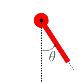
(A)

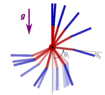
(B)

Figure 2: Single (A) and double (B) pendulums. Under torque bounds, these systems must swing back and forth several times before they can reach for the upright position, as depicted in (B) (lighter images represent earlier times).

3.2 Interpolation assumptions

We also require smoothness for the interpolated trajectories:

Assumption 3.

Interpolated trajectories $\gamma_{\textsf{int}}$ are smooth Lipschitz functions, and their time-derivatives $\dot{\gamma}_{\textsf{int}}$ (i.e. interpolated velocities) are also Lipschitz.

The following two assumptions ensure a continuous behaviour of the interpolation procedure:

Assumption 4 (Local boundedness).

Interpolated trajectories stay within a neighborhood of their start and end states, i.e. there exists a constant $\eta$ such that, for any $(x,x^{\prime})\in{\cal X}^{2}$, the interpolated trajectory $\gamma_{\textsf{int}}:~{}[0,\Delta t]\to{\cal C}$ resulting from $\textsc{INTERPOLATE}(x,x^{\prime})$ is included in a ball of center $x$ and radius $\eta\left\|x^{\prime}-x\right\|$.

Assumption 5 (Discrete-acceleration convergence).

When start and end states become close, accelerations of interpolated trajectories uniformly converge to the discrete acceleration between them, i.e. there exists some $\nu>0$ such that, if $\gamma_{\textsf{int}}:[0,\Delta t]\to{\cal C}$ results from $\textsc{INTERPOLATE}(x,x^{\prime})$, then

$$\forall\tau\in[0,\Delta t],\ \left\|\ddot{\gamma}_{\textsf{int}}(\tau)-\frac{\Delta{\dot{q}}}{\Delta t_{\textrm{disc}}}\right\|\ \leq\ \nu\left\|\Delta x\right\|,$$

where $\Delta t_{\textrm{disc}}:={\left\|\Delta q\right\|}/{\left\|{\dot{q}}\right\|}$.

Note that the expression $\frac{\Delta{\dot{q}}}{\Delta t_{\textrm{disc}}}$ above represents the discrete acceleration between $x$ and $x^{\prime}$. Its continuous analog would be $\frac{\left\|{\dot{q}}\right\|\,{\rm d}{{\dot{q}}}}{\left\|\,{\rm d}{q}\right\|}=\frac{\left\|{\dot{q}}\right\|\,{\rm d}{{\dot{q}}}}{\left\|{\dot{q}}\right\|\,{\rm d}{t}}=\frac{\,{\rm d}{{\dot{q}}}}{\,{\rm d}{t}}$.

These three assumptions ensure that the planner interpolates trajectories locally and “continuously” when $x$ and $x^{\prime}$ are close. We will call them altogether second-order continuity, where “second-order” refers to the discrete acceleration encoded in small variations $(\Delta q,\Delta{\dot{q}})$. This continuous behavior plays a key role in our proof of completeness, as it ensures that denser sampling will allow finding arbitrarily narrow state-space passages.

Let us consider again the example the double pendulum, for the interpolation function $\gamma=\textsc{INTERPOLATE}(x,x^{\prime})$ given by

$$\begin{array}[]{rcl}\gamma:[0,\Delta t]&\to&{\cal C}\\ t&\mapsto&\frac{\Delta{\dot{q}}}{2\Delta t}t^{2}+\left(\frac{\Delta q}{\Delta t}-\frac{\Delta{\dot{q}}}{2}\right)t+q.\end{array}$$ (5)

The duration $\Delta t$ is taken as $\Delta t_{{\textrm{disc}}}$, so that $\gamma(0)=q$, $\gamma(\Delta t)=q^{\prime}$ and $\ddot{\gamma}$ is the discrete acceleration. This interpolation, like any polynomial function, is Lipschitz smooth; Assumption 5 is verified by construction, and Assumption 4 can be checked as follows:

$$\left\|\gamma(t)-\gamma(0)\right\| \leq t\left\|\frac{1}{2}\frac{\Delta{\dot{q}}}{\Delta t}t+\frac{\Delta q}{\Delta t}-\frac{\Delta{\dot{q}}}{2}\right\|$$

$$\leq \Delta t\left\|\frac{\Delta{\dot{q}}}{2\Delta t}t+\frac{\Delta q}{\Delta t}-\frac{\Delta{\dot{q}}}{2}\right\|$$

$$\leq \frac{3}{2}\left\|\Delta{\dot{q}}\right\|\Delta t+\left\|\Delta q\right\|$$

$$\leq \left\|\Delta q\right\|\left(1+\frac{\left\|\Delta{\dot{q}}\right\|}{\left\|{\dot{q}}\right\|}\right)$$

$$\leq \left\|\Delta q\right\|\left(1+o_{\left\|\Delta x\right\|}(1)\right).$$

3.3 Completeness theorem

In order to prove the theorem, we will use the following two lemmas, which are proved in A.

Lemma 1.

Let $g:[0,\Delta t]\to\mathbb{R}^{k}$ denote a smooth Lipschitz function. Then, for any $(t,t^{\prime})\in[0,\Delta t]^{2}$,

$$\ \left\|\dot{g}(t)-\frac{g(t^{\prime})-g(t)}{|t^{\prime}-t|}\right\|\ \leq\ \frac{K_{g}}{2}|t^{\prime}-t|.$$

Lemma 2.

If there exists an admissible trajectory $\gamma$ with $\delta$-clearance in control space, then there exists $\delta^{\prime}<\delta$ and a neighboring admissible trajectory $\gamma^{\prime}$ with $\delta^{\prime}$-clearance in control space whose acceleration never vanishes, i.e. such that $\|\ddot{\gamma}^{\prime}\|$ is always greater than some constant $\ddot{m}>0$.

We can now state our main theorem:

Theorem 1.

Consider a time-invariant differential system (1) with Lipschitz-continuous $f$ and full actuation over a compact set of admissible controls ${{\cal U}_{\textsf{adm}}}$. Suppose that the kinodynamic planning problem between two states $x_{\textit{init}}$ and $x_{\textit{goal}}$ admits a smooth Lipschitz solution $\gamma:[0,T]\to{\cal C}$ with $\delta$-clearance in control space. A randomized motion planner (Algorithm 1) using a second-order continuous interpolation is probabilistically complete.

Proof. Let $\gamma:[0,\Delta t]\to{\cal C},t\mapsto\gamma(t)$ denote a smooth Lipschitz admissible trajectory from $x_{\textit{init}}$ to $x_{\textit{goal}}$, and $u:[0,\Delta t]\to{{\cal U}_{\textsf{adm}}}$ its associated control trajectory with $\delta$-clearance in control space. Consider two states $x=(q,{\dot{q}})$ and $x^{\prime}=(q^{\prime},{\dot{q}}^{\prime})$, as well as their corresponding time instants on the trajectory

$$t := \arg\min_{t}\left\|(\gamma(t),\dot{\gamma}(t))-x\right\|,$$

$$t^{\prime} := \arg\min_{t}\left\|(\gamma(t),\dot{\gamma}(t))-x^{\prime}\right\|.$$

Supposing without loss of generality that $t^{\prime}>t$, we denote by $\Delta t=t^{\prime}-t$ and $\Delta t_{\textrm{disc}}=\left\|{\dot{q}}\right\|/\left\|\Delta q\right\|$. Given a sufficiently dense sampling of the state space, we suppose that $\textrm{dist}_{\gamma}(x)\leq\rho$ and $\textrm{dist}_{\gamma}(x^{\prime})\leq\rho$ for a radius $\rho$ such that $\rho/\Delta t=O(\Delta t)$ and $\rho/\Delta t_{\textrm{disc}}=O(\Delta t)$; i.e. the radius $\rho$ is quadratic in the time difference.

Let $\gamma_{\textsf{int}}:[0,\Delta t]\to{\cal C}$ denote the result of the interpolation between $x$ and $x^{\prime}$. For $\tau\in[0,\Delta t]$, the torque required to follow the trajectory $\gamma_{\textsf{int}}$ is $u_{\textsf{int}}(\tau):=f(\gamma_{\textsf{int}}(\tau),\dot{\gamma}_{\textsf{int}}(\tau),\ddot{\gamma}_{\textsf{int}}(\tau))$. Since $u$ has $\delta$-clearance in control space,

$$\left|u_{\textsf{int}}(\tau)\right| \leq \left|u_{\textsf{int}}(\tau)-u(t)\right|+\left|u(t)\right|$$

$$\leq \left|f(\gamma_{\textsf{int}}(\tau),\dot{\gamma}_{\textsf{int}}(\tau),\ddot{\gamma}_{\textsf{int}}(\tau))-f(\gamma(t),\dot{\gamma}(t),\ddot{\gamma}(t))\right|+(1-\delta)\,\tau_{\textsf{max}},$$

(As previously, vector inequalities are component-wise.) Let us denote by $|\widetilde{u_{\textsf{int}}}|$ the first term of this inequality. We will now show that $|\widetilde{u_{\textsf{int}}}|=O(\Delta t)\to 0$ when $\Delta t\to 0$, and therefore that $|u_{\textsf{int}}(\tau)|\leq\tau_{\textsf{max}}$ for a small enough $\Delta t$ (i.e. when sampling density is high enough). Let us first rewrite it as follows:

$$|\widetilde{u_{\textsf{int}}}| = \left|f(\gamma_{\textsf{int}}(\tau),\dot{\gamma}_{\textsf{int}}(\tau),\ddot{\gamma}_{\textsf{int}}(\tau))-f(\gamma(t),\dot{\gamma}(t),\ddot{\gamma}(t))\right|$$

$$\leq \left\|f(\gamma_{\textsf{int}}(\tau),\dot{\gamma}_{\textsf{int}}(\tau),\ddot{\gamma}_{\textsf{int}}(\tau))-f(\gamma(t),\dot{\gamma}(t),\ddot{\gamma}(t))\right\|_{\infty}$$

$$\leq K_{f}\left\|(\gamma_{\textsf{int}}(\tau),\dot{\gamma}_{\textsf{int}}(\tau))-(\gamma(t),\dot{\gamma}(t))\right\|+K_{f}\left\|\ddot{\gamma}_{\textsf{int}}(\tau)-\ddot{\gamma}(t)\right\|$$

$$\leq \underbrace{K_{f}\left[(\eta+\nu)\left\|\Delta x\right\|+\textrm{dist}_{\gamma}(x)\right]}_{\text{position-velocity term (PV)}}+\underbrace{K_{f}\left\|\frac{\left\|{\dot{q}}\right\|}{\left\|\Delta q\right\|}\Delta{\dot{q}}-\ddot{\gamma}(t)\right\|}_{\text{acceleration term (A)}}.$$

The replacement of the norm $\left\|\cdot\right\|$ by $\left\|\cdot\right\|_{\infty}$ is possible because all norms of $\mathbb{R}^{n}$ are equivalent (a change in norm will be reflected by a different constant $K_{f}$). The transition from the second to the third row uses Lipschitz smoothness of $f$, as well as the triangular inequality to separate position-velocity and acceleration coordinates. The transition from the third to the fourth row relies on the two interpolation assumptions: local boundedness (yields the $\eta$ factor in the distance term) and convergence to the discrete-acceleration (yields the $\nu$ factor in the distance term, as well as the acceleration term).

The position-velocity term (PV) satisfies:

$$(\text{D})\ \leq\ (2\rho+\left\|\Delta\gamma\right\|)(\eta+\nu)+\rho\ \leq\ \frac{1}{2}K_{\gamma}(\eta+\nu)\Delta t+(1+2(\eta+\nu))\rho.$$

Since $\rho=O(\Delta t)$, we have $(\text{PV})=O(\Delta t)$ and thus $|\widetilde{u}|\leq(\text{A})+O(\Delta t)$. Next, the difference (A) can be bounded as:

$$(\text{A}) \leq \underbrace{\left\|\Delta{\dot{q}}\frac{\left\|{\dot{q}}\right\|}{\left\|\Delta q\right\|}-\Delta\dot{\gamma}\frac{\left\|\dot{\gamma}(t)\right\|}{\left\|\Delta\gamma\right\|}\right\|}_{(\Delta)}+\underbrace{\frac{\left\|\Delta\dot{\gamma}\right\|}{\left\|\Delta\gamma\right\|}\left|\left\|\dot{\gamma}(t)\right\|-\frac{\left\|\Delta\gamma\right\|}{\Delta t}\right|}_{\text{(A')}}$$

$$+ \underbrace{\left\|\frac{\Delta\dot{\gamma}}{\Delta t}-\ddot{\gamma}(t)\right\|.}_{\text{(A'')}}$$

From Lemma 1, the two terms (A’) and (A”) satisfy:

$$(\text{A'}) \leq \frac{K_{\dot{\gamma}}}{2}\frac{\left\|\Delta\dot{\gamma}\right\|}{\left\|\Delta\gamma\right\|}\Delta t\ =\ O(\Delta t),$$

$$(\text{A''}) \leq \frac{K_{\dot{\gamma}}}{2}\Delta t\ =\ O(\Delta t),$$

where the first upper bound $O(\Delta t)$ comes from the fact that $\frac{\left\|\Delta\dot{\gamma}\right\|}{\left\|\Delta\gamma\right\|}\underset{\Delta t\to 0}{\sim}\Delta t$. We now have $|\widetilde{u}|\leq(\Delta)+O(\Delta t)$. The term ($\Delta$) can be seen as the deviation between the discrete accelerations of $\gamma_{\textsf{int}}$ and $\gamma$. Let us decompose it in terms of norm and angular deviations:

$$(\Delta) \leq \left\|\left(\frac{\Delta\dot{\gamma}}{\left\|\Delta\dot{\gamma}\right\|}-\frac{\Delta{\dot{q}}}{\left\|\Delta{\dot{q}}\right\|}\right)\frac{\left\|\dot{\gamma}\right\|\left\|\Delta\dot{\gamma}\right\|}{\left\|\Delta\gamma\right\|}+\frac{\Delta{\dot{q}}}{\left\|\Delta{\dot{q}}\right\|}\left(\frac{\left\|\Delta\dot{\gamma}\right\|\left\|\dot{\gamma}\right\|}{\left\|\Delta\gamma\right\|}-\frac{\left\|\Delta{\dot{q}}\right\|\left\|{\dot{q}}\right\|}{\left\|\Delta q\right\|}\right)\right\|$$

$$\leq \underbrace{2\frac{\left\|\dot{\gamma}\right\|\left\|\Delta\dot{\gamma}\right\|}{\left\|\Delta\gamma\right\|}\left(1-\cos\widehat{(\Delta{\dot{q}},\Delta\dot{\gamma})}\right)}_{\text{angular deviation term ($\theta$)}}+\underbrace{\left|\frac{\left\|\dot{\gamma}\right\|\left\|\Delta\dot{\gamma}\right\|}{\left\|\Delta\gamma\right\|}-\frac{\left\|\Delta{\dot{q}}\right\|\left\|{\dot{q}}\right\|}{\left\|\Delta q\right\|}\right|}_{\text{norm deviation term (N)}}$$

The factor $\frac{2\left\|\dot{\gamma}\right\|\left\|\Delta\dot{\gamma}\right\|}{\left\|\Delta\gamma\right\|}$ before $(\theta)$ is $O(1)$ when $\Delta t\to 0$, while simple vector geometry then shows that

$$\sin\widehat{(\Delta{\dot{q}},\Delta\dot{\gamma})}\ \leq\ \frac{\textrm{dist}_{\gamma}(x)+\textrm{dist}_{\gamma}(x^{\prime})}{\left\|\Delta\dot{\gamma}\right\|}\ \leq\ \frac{\rho}{\ddot{m}\Delta t},$$

where $\ddot{m}:=\min_{t}\left\|\ddot{\gamma}(t)\right\|$. From Lemma 2, we can assume this minimum acceleration to be strictly positive. Then, it follows from $\rho=O(\Delta t^{2})$ that the sine above is $O(\Delta t)$. Recalling the fact that $1-\cos\theta<\sin\theta$ for any $\theta\in[0,\pi/2]$, we have $(\theta)=O(\Delta t)$.

Finally,

$$(\text{N}) \leq \frac{\left\|\Delta\dot{\gamma}\right\|}{\left\|\Delta\gamma\right\|}\left|\left\|\dot{\gamma}\right\|-\left\|{\dot{q}}\right\|\right|+\left\|{\dot{q}}\right\|\left|\frac{\left\|\Delta\dot{\gamma}\right\|}{\left\|\Delta\gamma\right\|}-\frac{\left\|\Delta{\dot{q}}\right\|}{\left\|\Delta q\right\|}\right|$$

$$\leq O(\Delta t\cdot\rho)+\left\|{\dot{q}}\right\|\frac{(\left\|\Delta q\right\|+\left\|\Delta{\dot{q}}\right\|)\,O(\rho)}{\left\|\Delta q\right\|(\left\|\Delta q\right\|+O(\rho))}$$

$$\leq O(\Delta t\cdot\rho)+\frac{\left\|{\dot{q}}\right\|\rho}{\left\|\Delta q\right\|+O(\rho)}+\frac{\|{\dot{q}}\|\left\|\Delta{\dot{q}}\right\|}{\left\|\Delta q\right\|}\frac{O(\rho)}{\left\|\Delta q\right\|+O(\rho)}$$

Where we used the fact that $\left\|\Delta\gamma\right\|\leq\textrm{dist}_{\gamma}(x)+\left\|\Delta q\right\|+\textrm{dist}_{\gamma}(x^{\prime})=\left\|\Delta q\right\|+O(\rho)$, and similarly for $\|\Delta\dot{\gamma}\|$. Because $\|\Delta q\|=\|{\dot{q}}\|\Delta t_{\textrm{disc}}+O(\Delta t_{\textrm{disc}}^{2})$ and $\rho/\Delta t_{\textrm{disc}}=O(\Delta t)$, the last two fractions are $O(\Delta t)$, so our last term $(\text{N})=O(\Delta t)$.

Overall, we have derived an upper bound $|u(\tau)|\leq(1-\delta)\tau_{\textsf{max}}+O(\Delta t)$. As a consequence, there exists a constant $\delta t>0$ such that, whenever $\Delta t\leq\delta t$, interpolated torques satisfy $|u|\leq\tau_{\textsf{max}}$ and the interpolated trajectory $\gamma_{\textsf{int}}=\textsc{INTERPOLATE}(x,x^{\prime})$ is admissible. Note that the constant $\delta t$ is uniform, in the sense that it does not depend on the index $t$ on the trajectory.

Conclusion of the Proof

We have effectively constructed the attraction sequence conjectured in [6]. We can now conclude the proof similarly to the strategy sketched in that paper. Let us denote by ${\cal B}_{t}:={\cal B}((\gamma,\dot{\gamma})(t),\delta\rho)$, the ball of radius $\delta\rho$ centered on $(\gamma,\dot{\gamma})(t)\in{\cal X}$, where $\delta\rho=O(\delta t^{2})$ as before. Suppose that the roadmap contains a state $x\in{\cal B}_{t}$, and let $t^{\prime}:=t+\delta t$. If the planner samples a state $x^{\prime}\in{\cal B}_{t^{\prime}}$, the interpolation between $x$ and $x^{\prime}$ will be successful and $x^{\prime}$ will be added to the roadmap. Since the volume of ${\cal B}_{t^{\prime}}$ is non-zero, the event $\{\textsc{SAMPLE}({{\cal X}}_{\textit{free}})\in{\cal B}_{t^{\prime}}\}$ will happen with probability one as the number of extensions goes to infinity. At the initialization of the planner, the roadmap is reduced to $x_{\textit{init}}=(\gamma(0),\dot{\gamma}(0))$. Therefore, using the property above, by induction on the number of time steps $\delta t$, the last state $x_{\textit{goal}}=(\gamma(T),\dot{\gamma}(T))$ will be eventually added to the roadmap with probability one, and the planner will find an admissible trajectory connecting $x_{\textit{init}}$ to $x_{\textit{goal}}$. $\blacksquare$

4 Completeness and state-based steering in practice

Shkolnik et al. [17] showed how RRTs could not be directly applied to kinodynamic planning due to their poor expansion rate at the boundaries of the roadmap. They illustrated this phenomenon on the planning problem of swinging up a (single) pendulum vertically against gravity. Let us consider the same system, i.e. the 1-DOF single pendulum depicted in Figure 2 (A), with length $l=20$ cm and mass $m=8$ kg. It satisfies the system assumptions of Theorem 1 a fortiori, as we saw that they apply to the double pendulum.

We assume that the single actuator of the pendulum, corresponding to the joint angle $\theta$ in Figure 2, has limited actuation power: $|\tau|\leq\tau_{\max}$. The static equilibrium of the system requiring the most torque is given at $\theta=\pm\pi/2$ with $\tau=\frac{1}{2}lmg\approx 7.84$ Nm. Therefore, when $\tau_{\max}<7.84$ Nm, it is impossible for the system to raise upright directly, and the pendulum rather needs to swing back and forth to accumulate kinetic energy before it can swing up. For any $\tau_{\max}>0$, the pendulum can achieve the swingup in a finite number of swings $N$, with $N\to\infty$ as $\tau_{\max}\to 0$.

4.1 Bezier interpolation

A common solution [25, 26, 27] to connect two states $(q,{\dot{q}})$ and $(q^{\prime},{\dot{q}}^{\prime})$ is the cubic Bezier curve (also called “Hermit curve”) which is the quadratic function $B(t)$ such that $B(0)=q$, $\dot{B}(0)={\dot{q}}$, $B(T)=q^{\prime}$ and $\dot{B}(T)=q^{\prime}$, where $T$ is the fixed duration of the interpolated trajectory. Its expression is given by:

$$B(t)\ =\ \frac{-2\Delta q+T({\dot{q}}+{\dot{q}}^{\prime})}{T^{3}}\,t^{3}+\frac{3\Delta q-2{\dot{q}}-{\dot{q}}^{\prime}}{T^{2}}\,t^{2}+{\dot{q}}t+q$$

This interpolation is straightforward to implement, however it does not verify our Assumption 5, as for instance

$$\ddot{B}(0)\ =\frac{6\Delta q-4{\dot{q}}-2{\dot{q}}^{\prime}}{T^{2}}\ \xrightarrow{\Delta x\to 0}\ \frac{-6{\dot{q}}}{T^{2}}\ \neq\ 0.$$ (6)

Our proof of completeness does not apply to such interpolators: even though a feasible trajectory is sampled as closely as possible $(\Delta x\to 0)$, the interpolated acceleration will not approximate the smooth acceleration underlying the feasible trajectory.

Proposition 1.

A randomized motion planner interpolating pendulum trajectories by Bezier curves with a fixed duration $T$ cannot find non-quasi static solutions by increasing sampling density.

Proof.

When actuation power decreases, the pendulum needs to store kinetic energy in order to swing up, which implies that all swingup trajectories go through velocities $|\dot{\theta}|>\dot{\theta}_{\textrm{swingup}}(\tau_{\max})$. The function $\dot{\theta}_{\textrm{swingup}}$ increases to a positive limit $\dot{\theta}_{\textrm{swingup}}^{\textrm{lim}}$ as $\tau_{\max}\to 0$, where $\dot{\theta}_{\textrm{swingup}}^{\textrm{lim}}>\sqrt{8g/l}$ from energetic considerations. Yet, feasible accelerations are also bound by $|\ddot{\theta}|\leq K\tau_{\max}$ for some constant $K>0$. Combining both observations in (6) yields:

$$K\tau_{\max}\geq 6\frac{|\dot{\theta}|}{T^{2}}\ >\ 6\frac{\dot{\theta}_{\textrm{swingup}}(\tau_{\max})}{T^{2}}\quad\Rightarrow\quad\dot{\theta}_{\textrm{swingup}}(\tau_{\max})\leq\frac{KT^{2}}{6}\tau_{\max}.$$

Since the planner uses a constant $T$ and $\dot{\theta}_{\textrm{swingup}}$ increases to $\dot{\theta}_{\textrm{swingup}}^{\textrm{lim}}>\sqrt{8g/l}$ when $\tau_{\max}$ decreases to 0, this inequality cannot be satisfied for arbitrary small actuation power $\tau_{\max}$. Hence, even with an arbitrarily high sampling density around a feasible trajectory $\gamma(t)$, the planner will not be able to reconstruct a feasible approximation $\gamma_{\textsf{int}}(t)$. ∎

4.2 Second-order continuous interpolation

Let ${\dot{q}}_{\textrm{avg}}:=\frac{1}{2}({\dot{q}}+{\dot{q}}^{\prime})$ denote the average velocity between $(q,{\dot{q}})$ and $(q^{\prime},{\dot{q}}^{\prime})$. Since the system has only one degree of freedom, one can interpolate trajectories that comply with our Assumption 5 using constant accelerations with a suitable trajectory duration:

$$\begin{array}[]{rcl}C:[0,\Delta t_{C}]&\to&]-\pi,\pi]\\ t&\mapsto&C(t)=q+t{\dot{q}}+\frac{t^{2}}{2}(\Delta{\dot{q}}/\Delta t_{C}).\end{array}$$

One can check that choosing $\Delta t_{C}=(\Delta q/{\dot{q}}_{\textrm{avg}})$ results in $\dot{C}(0)={\dot{q}}$, $\dot{C}(\Delta t_{C})={\dot{q}}^{\prime}$, $C(0)=q$ and $C(\Delta t_{C})=q^{\prime}$. This duration is similar to the term $\Delta t_{\textrm{disc}}$ in Assumption 5, with both expressions converging to the same value as $\Delta x\to 0$. We call $C(t)$ the second-order continuous 1-DOF (SOC1) interpolation.

Note that this interpolation function only applies to single-DOF systems. For multi-DOF systems, the correct duration $\Delta t_{C}$ used to transfer from one state to another is different for each DOF, hence constant accelerations cannot be used. One can then apply optimization techniques [20, 28] or use a richer family of curves such as piecewise linear-quadratic segments [29].

4.3 Comparison in simulations

According to Theorem 1 and our previous discussion, a randomized planner based on Bezier interpolation is not expected to be probabilistically complete as $\tau_{\max}\to 0$, while the same planner using the SOC1 interpolation will be complete at any rate. We asserted this statement in simulations of the pendulum with RRT [30].

Our implementation of RRT is that described in Algorithm 1, with the addition of the steer-to-goal heuristic: every $m=100$ steps, the planner tries to steer to $x_{\textit{goal}}$ rather than $x_{\textit{rand}}$. This extra step speeds up convergence when the system reaches the vicinity of the goal area. We use uniform random sampling for $\textsc{SAMPLE}(S)$, while for $\textsc{PARENTS}(x^{\prime},V)$ returns the $k=10$ nearest neighbors of $x^{\prime}$ in the roadmap $V$. All the source code used in these experiments can be accessed at [31].

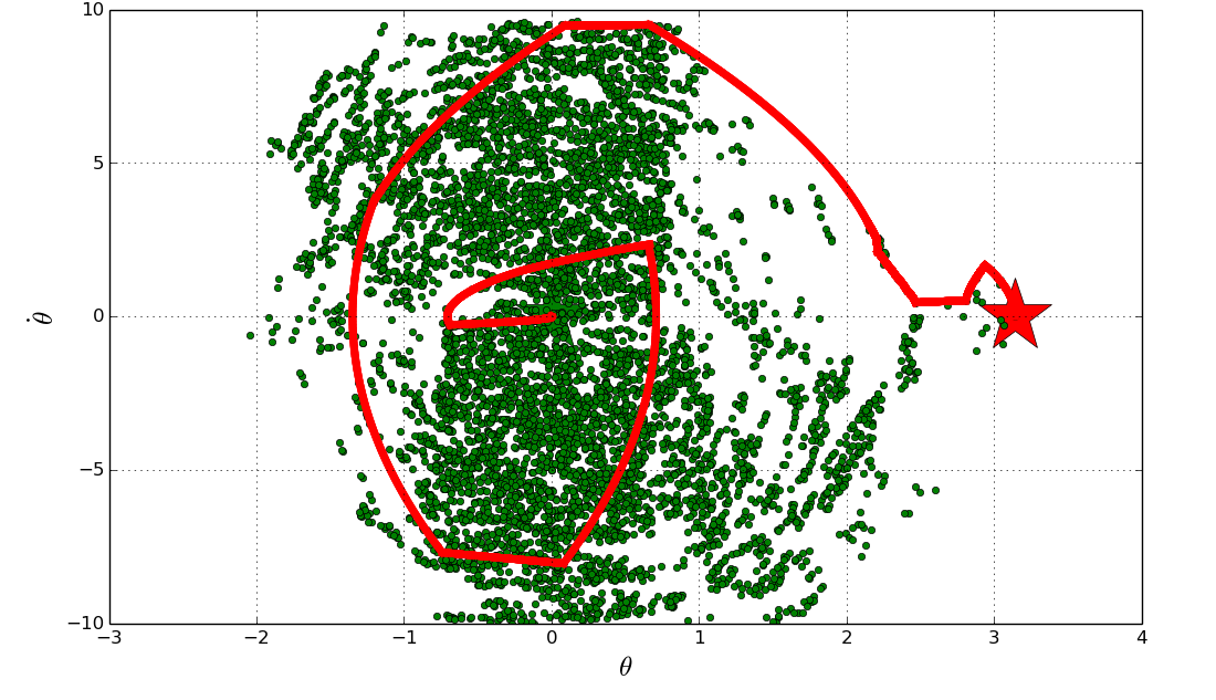
Figure 3: Phase-space portrait of the roadmap constructed by RRT using the second-order continuous (SOC1) interpolation. The planner found a successful trajectory (red line) after 26,300 extensions. This planner is probabilistically complete (Theorem 1) thanks to the fact that SOC1 curves satisfy Assumption 5.

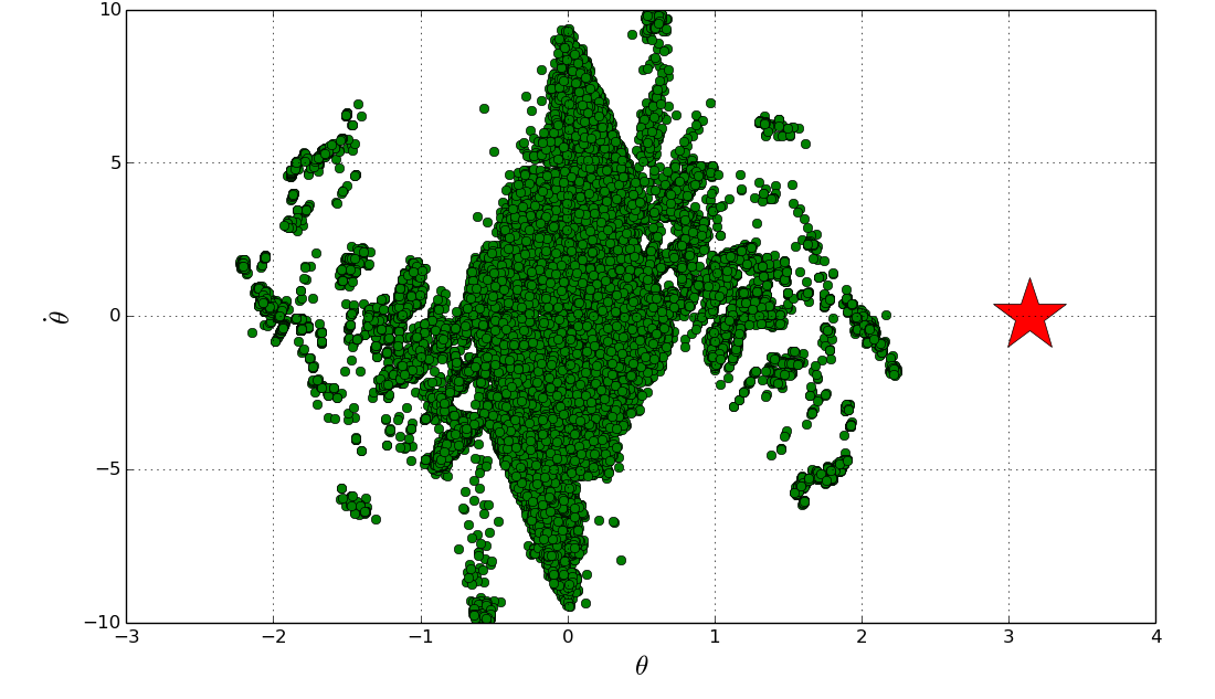
Figure 4: Roadmap constructed by RRT after 100,000 extensions using the Bezier interpolation. Reachable states are distributed in two major areas: a central, diamond shape corresponding to the states that the planner can connect at any rate, and two cones directed towards the goal ($\theta=\pi$ or $\theta=-\pi$). Even after several days of computations, this planner could not find a successful motion plan. Our completeness theorem does not apply to this planner because Bezier curves do not satisfy Assumption 5.

We compared the performance of RRT with the Bezier and SOC1 interpolations, all other parameters being the same, on a single pendulum with $\tau_{\max}=5$ Nm. The RRT-SOC1 combo found a four-swing solution after 26,300 RRT extensions, building a roadmap with 6434 nodes (Figure 3).

Meanwhile, even after one day of computations and more than 200,000 RRT extensions, the RRT-Bezier combo could not find any solution. Figure 4 shows the roadmap at 100,000 extensions (26,663 nodes). Interestingly, we can distinguish two zones in this roadmap. The first one is a dense, diamond-shape area near the downward equilibrium $\theta=0$. It corresponds to states that are straightforward to connect by Bezier interpolation, and as expected from Proposition 1, velocities $\dot{\theta}$ in this area decrease sharply with $\theta$. The second one consists of two cones directed torwards the goal. Both areas exhibit a higher density near the axis $\dot{\theta}=0$, which is also consistent with Proposition 1.

The comparison of the two roadmaps is clear: with a second-order continuous interpolation, the RRT-SOC1 planner leverages additional sampling into exploration of the state space. Conversely, RRT-Bezier lacks this property (Proposition 1), and its roadmap stays confined to a subset of the pendulum’s reachable space.

5 Conclusion

In this paper, we provided the first “operational” proof of probabilistic completeness for a large class of randomized kinodynamic planners, namely those that interpolate state-space trajectories. We observed that an important ingredient for completeness is the “continuity” of the interpolation procedure, which we characterized by the second-order continuity (SOC) property. In particular, we found in simulation experiments that this property is critical to planner performances: a standard RRT with second-order continuous interpolation has no difficulty finding swingup trajectories for a low-torque pendulum, while the same RRT with Bezier interpolation (which are not SOC) could not find any solution. This experimentally confirms our completeness theorem and suggests that second-order continuity is an important design guideline for kinodynamic planners with state-based steering.

References

Appendix A Proofs of the lemmas

Lemma 1.

Let $g:[0,\Delta t]\to\mathbb{R}^{k}$ denote a smooth Lipschitz function. Then, for any $(t,t^{\prime})\in[0,\Delta t]^{2}$,

$$\ \left\|\dot{g}(t)-\frac{g(t^{\prime})-g(t)}{|t^{\prime}-t|}\right\|\ \leq\ \frac{K_{g}}{2}|t^{\prime}-t|.$$

Proof.

For $t^{\prime}>t$,

$$\left\|\dot{g}(t)-\frac{g(t^{\prime})-g(t)}{t^{\prime}-t}\right\| \leq \frac{1}{t^{\prime}-t}\left\|\int_{t}^{t^{\prime}}(\dot{g}(t)-\dot{g}(w))\,{\rm d}{w}\right\|$$

$$\leq \frac{1}{t^{\prime}-t}\int_{t}^{t^{\prime}}\left\|\dot{g}(t)-\dot{g}(w)\right\|\,{\rm d}{w}$$

$$\leq \frac{K_{g}}{t^{\prime}-t}\int_{t}^{t^{\prime}}|t-w|\,{\rm d}{w}$$

$$\leq \frac{K_{g}}{2}(t^{\prime}-t).\qed$$

Lemma 2.

If there exists an admissible trajectory $\gamma$ with $\delta$-clearance in control space, then there exists $\delta^{\prime}<\delta$ and a neighboring admissible trajectory $\gamma^{\prime}$ with $\delta^{\prime}$-clearance in control space which is always accelerating, i.e. such that $\|\ddot{\gamma}^{\prime}\|$ is always greater than some constant $\ddot{m}>0$.

Proof.

If there is a time interval $[t,t^{\prime}]$ on which $\ddot{\gamma}\equiv 0$, suffices to add a wavelet function $\delta\ddot{\gamma}_{i}$ of arbitrary small amplitude $\delta{\ddot{q}}_{i}$ and zero integral over $[t,t^{\prime}]$ to generate a new trajectory $\ddot{\gamma}+\delta\ddot{\gamma}$ where the acceleration cancels on at most a discrete number of time instants. Adding accelerations $\delta\ddot{\gamma}_{i}$ directly is possible thanks to full actuation, while $\delta^{\prime}$-clearance can be achieved for $\delta^{\prime}\leq\delta$ by taking sufficiently small amplitudes $\delta{\ddot{q}}_{i}$.

Suppose now that the roots of $\ddot{\gamma}$ form a discrete set $\{t_{0},t_{1},\ldots,t_{m}\}$. Let $t_{0}$ be one of these roots, and let $[t,t^{\prime}]$ denote a neighbordhood of $t_{0}$. Repeat the process of adding wavelet functions $\delta\ddot{\gamma}_{i}$ and $\delta\ddot{\gamma}_{j}$ of zero integral over $[t,t^{\prime}]$ and arbitrary small amplitude to two coordinates $i$ and $j$, but this time enforcing that the sum of the two wavelets satisfies $|\delta\ddot{\gamma}_{i}+\delta\ddot{\gamma}_{j}|\geq\epsilon_{ij}>0$. This method ensures that the root $t_{0}$ is eliminated (either $\ddot{\gamma}_{i}(t_{0})\neq 0$ or $\ddot{\gamma}_{j}(t_{0})\neq 0$) without introducing new roots. We conclude by iterating the process on the finite set of roots. ∎

References

- [1] S. Caron, Q.-C. Pham, Y. Nakamura, Completeness of randomized kinodynamic planners with state-based steering, in: Robotics and Automation (ICRA), 2014 IEEE International Conference on, IEEE, 2014, pp. 5818–5823.
- [2] J.-C. Latombe, Robot motion planning, Vol. 124, Springer US, 1991.
- [3] S. LaValle, Planning algorithms, Cambridge Univ Press, 2006.
- [4] L. E. Kavraki, P. Svestka, J.-C. Latombe, M. H. Overmars, Probabilistic roadmaps for path planning in high-dimensional configuration spaces, Robotics and Automation, IEEE Transactions on 12 (4) (1996) 566–580.
- [5] D. Hsu, R. Kindel, J.-C. Latombe, S. Rock, Randomized kinodynamic motion planning with moving obstacles, The International Journal of Robotics Research 21 (3) (2002) 233–255.
- [6] S. M. LaValle, J. J. Kuffner, Randomized kinodynamic planning, The International Journal of Robotics Research 20 (5) (2001) 378–400.
- [7] S. Karaman, E. Frazzoli, Sampling-based algorithms for optimal motion planning, The International Journal of Robotics Research 30 (7) (2011) 846–894.
- [8] D. Hsu, J.-C. Latombe, R. Motwani, Path planning in expansive configuration spaces, in: Robotics and Automation, 1997. Proceedings., 1997 IEEE International Conference on, Vol. 3, IEEE, 1997, pp. 2719–2726.
- [9] T. Lozano-Perez, Spatial planning: A configuration space approach, Computers, IEEE Transactions on 100 (2) (1983) 108–120.
- [10] B. Donald, P. Xavier, J. Canny, J. Reif, Kinodynamic motion planning, Journal of the ACM (JACM) 40 (5) (1993) 1048–1066.
- [11] J.-P. Laumond, Robot Motion Planning and Control, Springer-Verlag, New York, 1998.
- [12] F. Bullo, K. M. Lynch, Kinematic controllability for decoupled trajectory planning in underactuated mechanical systems, Robotics and Automation, IEEE Transactions on 17 (4) (2001) 402–412.
- [13] J. Bobrow, S. Dubowsky, J. Gibson, Time-optimal control of robotic manipulators along specified paths, The International Journal of Robotics Research 4 (3) (1985) 3–17.
- [14] P.-B. Wieber, On the stability of walking systems, in: Proceedings of the international workshop on humanoid and human friendly robotics, 2002.
- [15] S. Caron, Q.-C. Pham, Y. Nakamura, Leveraging cone double description for multi-contact stability of humanoids with applications to statics and dynamics, in: Robotics: Science and System, 2015.
- [16] J. Bialkowski, M. Otte, E. Frazzoli, Free-configuration biased sampling for motion planning, in: Intelligent Robots and Systems (IROS), 2013 IEEE/RSJ International Conference on, IEEE, 2013, pp. 1272–1279.
- [17] A. Shkolnik, M. Walter, R. Tedrake, Reachability-guided sampling for planning under differential constraints, in: Robotics and Automation, 2009. ICRA’09. IEEE International Conference on, IEEE, 2009, pp. 2859–2865.
- [18] G. Papadopoulos, H. Kurniawati, N. M. Patrikalakis, Analysis of asymptotically optimal sampling-based motion planning algorithms for lipschitz continuous dynamical systems, arXiv preprint arXiv:1405.2872.
- [19] T. Kunz, M. Stilman, Probabilistically complete kinodynamic planning for robot manipulators with acceleration limits, in: Intelligent Robots and Systems (IROS 2014), 2014 IEEE/RSJ International Conference on, IEEE, 2014, pp. 3713–3719.
- [20] A. Perez, R. Platt, G. Konidaris, L. Kaelbling, T. Lozano-Perez, Lqr-rrt*: Optimal sampling-based motion planning with automatically derived extension heuristics, in: Robotics and Automation (ICRA), 2012 IEEE International Conference on, IEEE, 2012, pp. 2537–2542.
- [21] R. Tedrake, Lqr-trees: Feedback motion planning on sparse randomized trees.
- [22] T. Kunz, M. Stilman, Kinodynamic rrts with fixed time step and best-input extension are not probabilistically complete, in: Algorithmic Foundations of Robotics XI, Springer, 2015, pp. 233–244.
- [23] S. Karaman, E. Frazzoli, Optimal kinodynamic motion planning using incremental sampling-based methods, in: Decision and Control (CDC), 2010 49th IEEE Conference on, IEEE, 2010, pp. 7681–7687.
- [24] S. Karaman, E. Frazzoli, Sampling-based optimal motion planning for non-holonomic dynamical systems, in: IEEE Conference on Robotics and Automation (ICRA), 2013.
- [25] K. Jolly, R. S. Kumar, R. Vijayakumar, A bezier curve based path planning in a multi-agent robot soccer system without violating the acceleration limits, Robotics and Autonomous Systems 57 (1) (2009) 23–33.
- [26] I. Škrjanc, G. Klančar, Optimal cooperative collision avoidance between multiple robots based on bernstein–bézier curves, Robotics and Autonomous systems 58 (1) (2010) 1–9.
- [27] K. Hauser, Fast interpolation and time-optimization on implicit contact submanifolds., in: Robotics: Science and Systems, Citeseer, 2013.
- [28] Q.-C. Pham, S. Caron, Y. Nakamura, Kinodynamic planning in the configuration space via velocity interval propagation, Robotics: Science and System.
- [29] K. Hauser, V. Ng-Thow-Hing, Fast smoothing of manipulator trajectories using optimal bounded-acceleration shortcuts, in: Robotics and Automation (ICRA), 2010 IEEE International Conference on, IEEE, 2010, pp. 2493–2498.
- [30] S. M. LaValle, J. J. Kuffner Jr, Rapidly-exploring random trees: Progress and prospects.
- [31] Source code to be published online.