Geometric Lorenz flows with historic behavior

Abstract.

We will show that, in the the geometric Lorenz flow, the set of initial states which give rise to orbits with historic behavior is residual in a trapping region.

Consider a continuous map $\varphi:X\to X$ of a compact space $X$. We say that the forward orbit $O^{+}(x,\varphi)=\{x,\varphi(x),\varphi^{2}(x),\dots\}$ of $x\in X$ has historic behavior if the Birkhoff average $\lim_{n\to\infty}\frac{1}{n+1}\sum_{i=0}^{n}g(\varphi^{i}(x))$ does not exist for some continuous function $g:X\to\mathbb{R}$. The notion of historic behavior was introduced by Ruelle [Ru]. We say that a subset $A$ of $X$ is a historic initial set if, for any $x\in A$, the forward orbit $O^{+}(x,\varphi)$ has historic behavior. Jordan, Naudot and Young [JNY] showed that the convergence of every higher order average in [BDV, p. 11] is totally controlled by the presence of the historic initial sets.

Let $\varphi:\mathbb{S}\to\mathbb{S}$ be the doubling map on the circle $\mathbb{S}=\mathbb{R}/\mathbb{Z}$. Takens [Ta2] showed that there exists a residual historic initial set in $\mathbb{S}$. In fact, he presented only one orbit $O^{+}(x,\varphi)$ which is dense in $\mathbb{S}$ and has historic behavior. Then, by Dowker [Do], there exists a historic initial set which is residual in $\mathbb{S}$. Dowker’s theorem is very useful to show the existence of a residual historic initial set for various 1-dimensional maps. The quenched random dynamics version of Takens’ result is obtained by Nakano [Na]. Takens’ argument is applicable also to the Lorenz map $\alpha:[-1,1]\to[-1,1]$, see Remark 1.1. Many of such residual sets would have zero Lebesgue measure. On the other hand, for any integer $r$ with $2\leq r<\infty$, Kiriki and Soma [KS] proved that there exists a two-dimensional diffeomorphism which is arbitrarily $C^{r}$ close to a diffeomorphism with a quadratic homoclinic tangency and has a non-empty open historic initial set $D$. Note that the open set $D$ has positive 2-dimensional Lebesgue measure. Hence, in particular, this result gives an answer to Takens’ Last Problem [Ta2] in the $C^{2}$-persistent way (see [PT, Section 6.1] for the definition). Moreover, it suggests that, in certain classes of 2-dimensional diffeomorphisms, the historic initial set is not negligible from the physical point of view.

In this paper, we will study the historic behavior on flow dynamics. Let $x(t)_{t\geq 0}$ be a forward orbit of a flow on a compact space $X$. Then we say that the orbit has historic behavior if the the time average

$$\lim_{t\to\infty}\frac{1}{t}\int_{0}^{t}g(x(s))\,ds$$

does not exist for some continuous function $g:X\to\mathbb{R}$. See Takens [Ta1] for the definition. Bowen’s example given in [Ta1] is a flow on $\mathbb{R}^{2}$ which has a heteroclinic loop consisting of a pair of saddle points and two arcs connecting them. The loop bounds an open disk $D$ in $\mathbb{R}^{2}$ which contains a singular point $p$ of the flow such that the complement $D\setminus\{p\}$ is a historic initial set. However, this example is fragile in the sense that it is not persistent under perturbations which break the saddle connections. Very recently, Labouriau and Rodrigues [LR] present a persistent class of differential equations on $\mathbb{R}^{3}$ exhibiting historic behavior for an open set of initial conditions, which answers Takens’ Last Problem for 3-dimensional flows.

Here we consider the geometric Lorenz flow introduced by Guckenheimer [Gu] as a robust model which does not belong to classes in [LR]. Robinson [Ro] proved that the geometric Lorenz flow is preserved under $C^{2}$-perturbation. Note that Tucker [Tu] showed that the flow exhibited by the system of differential equations in Lorenz [Lo] (the original Lorenz flow) is realized by some geometric Lorenz model. Our main theorem (Theorem 2.1) of this paper proves that any geometric Lorenz flow satisfying the conditions in Section 1 has a residual historic initial set. On the other hand, Araujo et al [APPV] proved that, for any singular hyperbolic attractor of a 3-dimensional flow, the historic initial set in the topological basin of attractor has zero Lebesgue measure. Since the geometric Lorenz attractor is proved to be a singular hyperbolic attractor by [MPP], the historic initial set is negligible from the physical point of view. But, Theorem 2.1 implies that it is not the case in dynamical systems from the topological point of view.

Finally, we note that Dowker’s result does not work in flow dynamics. So, in our proof, we need to construct a residual historic initial set for the geometric Lorentz flow practically.

1. Preliminaries

First of all, we will review the geometric Lorentz flow briefly. See [Wi1, GW, Wi2] for details.

Consider the square $\Sigma=\{(x,y)\in\mathbb{R}^{2}\,;\,|x|,|y|\leq 1\}$ and the vertical segment $\Gamma=\{(0,y)\in\mathbb{R}^{2}\,;\,|y|\leq 1\}$ in $\Sigma$. Let $\Sigma_{\pm}$ be the components of $\Sigma\setminus\Gamma$ with $\Sigma_{\pm}\ni(\pm 1,0)$. A map $L:\Sigma\setminus\Gamma\to\Sigma$ is said to be a Lorenz map if it is a piecewise $C^{2}$ diffeomorphism which has the form

(1.1) $$L(x,y)=(\alpha(x),\beta(x,y)),$$

where $\alpha:[-1,1]\setminus\{0\}\to[-1,1]$ is a piecewise $C^{2}$-function with symmetric property $\alpha(-x)=-\alpha(x)$ and satisfying

(1.2) $$\lim_{x\rightarrow 0+}\alpha(x)=-1,\ \alpha(1)<1,\ \lim_{x\rightarrow 0+}\alpha^{\prime}(x)=\infty,\ \alpha^{\prime}(x)>\sqrt{2}$$

for any $x\in(0,1]$ (see Figure 1.1 (a)), and $\beta:\Sigma\setminus\Gamma\to[-1,1]$ is a contraction in the $y$-direction. Moreover, it is required that the images $L(\Sigma_{+})$, $L(\Sigma_{-})$ are mutually disjoint cusps in $\Sigma$, where the vertices $\boldsymbol{v}_{+}$, $\boldsymbol{v}_{-}$ of $L(\Sigma_{\pm})$ are contained in $\{\mp 1\}\times[-1,1]$ respectively (see Figure 1.1 (b)).

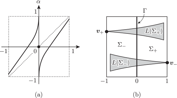
Figure 1.1.

Remark 1.1 (Historic behavior for the 1-dimensional Lorenz map).

We denote the forward orbit of $x\in[-1,1]$ under $\alpha$ by $O^{+}(x,\alpha)$. By Hofbauer [Ho], the dynamics of $\alpha$ on $[-1,1]$ is described by a Markov partition on finite symbols. Let $s^{\prime}$ be a periodic sequence of these symbols and $s^{\prime\prime}$ a sequence such that, for the point $x^{\prime\prime}$ of $[-1,1]$ corresponding to $s^{\prime\prime}$, the partial averages $\frac{1}{n+1}\sum_{i=0}^{n}\delta_{\alpha^{i}(x^{\prime\prime})}$ converge to the Lebesgue measure. As in Takens [Ta1, Section 4], there exists a sequence $s_{0}$ of these symbols in which long initial segments of $s^{\prime}$ and those of $s^{\prime\prime}$ appear alternately and such that, for the point $x_{0}$ of $I$ corresponding to $s_{0}$, $O^{+}(x_{0},\alpha)$ is dense in $[-1,1]$ and has historic behavior. Then, by Dowker [Do], there exists a historic initial set which is residual in $[-1,1]$.

We identify the square $\Sigma$ and any subset of $\Sigma$ with their images in $\mathbb{R}^{3}$ via the embedding $\iota:\mathbb{R}^{2}\to\mathbb{R}^{3}$ with $\iota(x,y)=(x,y,1)$. A $C^{2}$-vector field $X_{L}$ on $\mathbb{R}^{3}$ is said to be a geometric Lorenz vector field controlled by the Lorenz map $L:\Sigma\setminus\Gamma\to\Sigma$ (1.1) if it satisfies the following conditions (i) and (ii).

1. For any point $(x,y,z)$ in a neighborhood of the origin $\mathbf{0}$ of $\mathbb{R}^{3}$, $X_{L}$ is given by the differential equation

   (1.3) $$\dot{x}=\lambda x,\quad\dot{y}=-\mu y,\quad\dot{z}=-\nu z$$

   for some $\lambda>0$, $\mu>\nu>0$. Moreover, $\Gamma$ is contained in the stable manifold $W^{s}(\mathbf{0})$ of $\mathbf{0}$.

2. All forward orbits of $X$ starting from $\Sigma\setminus\Gamma$ will return to $\Sigma$ and the first return map is $L$.

Note then that $\mathbf{0}$ is a singular point (an equilibrium) of saddle type, the local unstable manifold of $\mathbf{0}$ is tangent to the $x$-axis, and the local stable manifold of $\mathbf{0}$ is tangent to the $yz$-plane, see Figure 1.2.

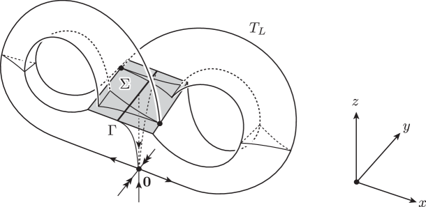
Figure 1.2.

The $C^{2}$-map $\varphi_{L}:\mathbb{R}^{3}\times\mathbb{R}\to\mathbb{R}^{3}$ defined by $\varphi_{L}(\boldsymbol{x},0)=\boldsymbol{x}$ and $(\partial/\partial t)\varphi_{L}(\boldsymbol{x},t)=X_{L}(\varphi_{L}(\boldsymbol{x},t))$ is called the geometric Lorenz flow associated with the vector field $X_{L}$. The closure of $\bigcup_{\boldsymbol{z}\in\Sigma\setminus\Gamma}\varphi_{L}(\boldsymbol{z},[0,\infty))$ in $\mathbb{R}^{3}$ is homeomorphic to a genus two handlebody as illustrated in Figure 1.2, which is called the trapping region of $\varphi_{L}$ and denoted by $T_{\varphi_{L}}$ or $T_{L}$. Any forward orbit for $\varphi_{L}$ with its initial point in $T_{L}$ cannot escape from $T_{L}$.

For simplicity, we suppose moreover that the geometric Lorenz flow satisfies the differential equation (1.3) on

$$V_{L}=T_{L}\cap[-0.1,0.1]\times[-1,1]\times[0,1].$$

In fact, this assumption is not crucial and our subsequent argument still works for any geometric Lorenz flow which satisfies (1.3) only on an arbitrarily small neighborhood of $\mathbf{0}$ in $T_{L}$.

2. Historic behavior for the geometric Lorenz flow

Let $\varphi_{L}$ be the geometric Lorenz flow given in the previous section. Suppose that $g:T_{L}\to\mathbb{R}$ is a continuous function on the trapping region $T_{L}$. For $\tau>0$ and $\delta>0$, the forward orbit $\varphi_{L}(\boldsymbol{x},t)_{t\geq 0}$ emanating from $\boldsymbol{x}\in T_{L}$ is said to have $(\tau,\delta)$-historic behavior with respect to $g$ if there exist $\tau_{0}$, $\tau_{1}$ with $\tau_{0},\tau_{1}\geq\tau$ such that

$$\left|\frac{1}{\tau_{0}}\int_{0}^{\tau_{0}}g(\varphi_{L}(\boldsymbol{x},t))\,dt-\frac{1}{\tau_{1}}\int_{0}^{\tau_{1}}g(\varphi_{L}(\boldsymbol{x},t))\,dt\,\right|\geq\delta.$$

In particular, $\varphi_{L}(\boldsymbol{x},t)_{t\geq 0}$ has historic behavior if and only if there exists $\delta>0$ and a continuous function $g$ on $T_{L}$ such that, for any $\tau>0$, $\varphi_{L}(\boldsymbol{x},t)_{t\geq 0}$ has $(\tau,\delta)$-historic behavior with respect to $g$.

For any $\boldsymbol{y},\boldsymbol{z}\in T_{L}$ contained in the same forward orbit $\varphi_{L}(\boldsymbol{x},[0,\infty))$ with $\boldsymbol{x}\in\Sigma$, the sub-arc of $\varphi_{L}(\boldsymbol{x},[0,\infty))$ connecting $\boldsymbol{y}$ with $\boldsymbol{z}$ is denoted by $\Phi_{L}(\boldsymbol{y},\boldsymbol{z})$ or $\Phi_{L}(\boldsymbol{z},\boldsymbol{y})$. Let $t_{\boldsymbol{x}}(\boldsymbol{y})\geq 0$ be the number with $\varphi_{L}(\boldsymbol{x},t_{\boldsymbol{x}}(\boldsymbol{y}))=\boldsymbol{y}$. We set $\tau(\boldsymbol{y},\boldsymbol{z})=|t_{\boldsymbol{x}}(\boldsymbol{y})-t_{\boldsymbol{x}}(\boldsymbol{z})|$. Note that $\tau(\boldsymbol{y},\boldsymbol{z})$ is independent of $\boldsymbol{x}\in\Sigma$ with $\varphi_{L}(\boldsymbol{x},[0,\infty))\ni\boldsymbol{y},\boldsymbol{z}$. We also set $\tau(\boldsymbol{y},\boldsymbol{z})=\tau(\gamma)$ if $\gamma=\Phi_{L}(\boldsymbol{y},\boldsymbol{z})$. Let $A$ be a compact subset of $T_{L}\setminus\{\mathbf{0}\}$ such that $\Phi_{L}(\boldsymbol{y},\boldsymbol{z})\cap A$ is a disjoint union of finitely many arcs $\gamma_{1},\dots,\gamma_{n}$. Then the total sum $\sum_{i=1}^{n}\tau(\gamma_{i})$ is denoted by $\tau(\boldsymbol{y},\boldsymbol{z})|_{A}$.

Take a periodic point $x_{\mathrm{per}(2)}$ of $\alpha$ with period two. Let $\pi:\mathbb{R}^{3}\to\mathbb{R}^{2}$ be the orthogonal projection defined by $\pi(x,y,z)=(x,z)$. For any point $\boldsymbol{x}$ of $\Sigma$ with $\boldsymbol{x}_{[1]}=x_{\mathrm{per}(2)}$, the the image $Q(x_{\mathrm{per}(2)})=\pi(\varphi_{L}(\boldsymbol{x},[0,\infty)))$ is a closed curve in the $xz$-plane disjoint from the origin of $\mathbb{R}^{2}$. Here we denote the first entry of an element $\boldsymbol{a}$ of $\mathbb{R}^{3}$ by $\boldsymbol{a}_{[1]}$, that is, $(a,b,c)_{[1]}=a$. Though $Q(x_{\mathrm{per}(2)})$ depends on $x_{\mathrm{per}(2)}$, it is independent of the $y$-entry of $\boldsymbol{x}$. See Figure 2.1.

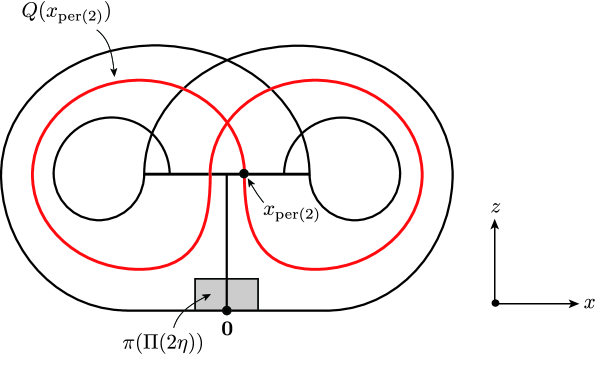
Figure 2.1.

For $\eta>0$, the rectangular solid $[-\eta,\eta]^{2}\times[0,\eta]$ is denoted by $\Pi(\eta)$. By taking the $\eta$ sufficiently small, one can suppose that $\Pi(\eta)\cap T_{L}\subset V_{L}$ and $\Pi(2\eta)\cap\varphi_{L}(\boldsymbol{x},[0,\infty))=\emptyset$ for any $\boldsymbol{x}\in\Sigma$ with $\boldsymbol{x}_{[1]}=x_{\mathrm{per}(2)}$. Consider the subspaces

$$\partial_{\mathrm{side}}\Pi(\eta)=\{-\eta,\eta\}\times[-\eta,\eta]\times[0,\eta]\quad\text{and}\quad\partial_{\mathrm{top}}\Pi(\eta)=[-\eta,\eta]^{2}\times\{\eta\}$$

of the boundary $\partial\Pi(\eta)$.

By the third equation of (1.3) on $V_{L}$, any sub-arc $\gamma$ of an orbit connecting $\Sigma$ with $\partial_{\mathrm{top}}\Pi(\eta)$ in $T_{L}\cap[-\eta,\eta]\times[-1,1]\times[\eta,1]\subset V_{L}$ satisfies

(2.1) $$\tau(\gamma)=\frac{\log(\eta^{-1})}{\nu}.$$

Note that the Lorenz flow does not have singular points in the compact set $\overline{T_{L}\setminus\Pi(\eta)}$, where $\overline{A}$ denotes the closure of a subset $A$ of $T_{L}$. It follows from the fact that there exists a constant $C>0$ satisfying

(2.2) $$\tau(\boldsymbol{x},L(\boldsymbol{x}))|_{\,\overline{T_{L}\setminus\Pi(\eta)}}\leq C$$

for any $\boldsymbol{x}\in\Sigma\setminus\Gamma$.

The following is our main theorem in this paper.

Theorem 2.1.

There exists a residual subset $\mathcal{H}$ of $\Sigma$ such that, for any $\boldsymbol{x}\in\mathcal{H}$, the forward orbit $\varphi_{L}(\boldsymbol{x},t)_{t\geq 0}$ has historic behavior.

Here we fix a continuous function $g:T_{L}\to\mathbb{R}$ satisfying the following condition.

1. $0\leq g(\boldsymbol{x})\leq 1$ for any $\boldsymbol{x}\in T_{L}$.

2. The support of $g$ is contained in $\Pi(2\eta)\cap T_{L}$ and $g(\boldsymbol{x})=1$ on $\Pi(\eta)\cap T_{L}$.

The following lemma is crucial in the proof of Theorem 2.1.

Lemma 2.2.

For any positive integer $N$, any $0<\varepsilon<1$ and $\boldsymbol{x}_{0}\in\Sigma$, there exists an open disk $U_{(\boldsymbol{x}_{0},N,\varepsilon)}$ contained in the $\varepsilon$-neighborhood of $\boldsymbol{x}_{0}$ in $\Sigma$ and satisfying the following condition.

1. For any $\boldsymbol{z}\in U_{(\boldsymbol{x}_{0},N,\varepsilon)}$, $\varphi_{L}(\boldsymbol{z},t)_{t\geq 0}$ has $(N,1/2)$-historic behavior with respect to $g$.

Here we note that the disk $U_{(\boldsymbol{x}_{0},N,\varepsilon)}$ is not necessarily required to have $x_{0}$ as an element.

Proof.

Since $0<\varepsilon<1$, $\lim_{\sigma\rightarrow\infty}\log(\varepsilon^{-\sigma})=\infty$. Thus one can have a constant $\sigma\geq 1$ satisfying

(2.3) $$\frac{1}{\lambda}\bigl{(}\log(\varepsilon^{-\sigma})+\log\eta\bigr{)}\geq\max\left\{N,\frac{6C\log(\varepsilon^{-1})}{\log 2}+\frac{4\log(\eta^{-1})}{\nu}\right\}.$$

Set $(\boldsymbol{x}_{0})_{[1]}=x_{0}$ and consider the interval $I(x_{0},\varepsilon)=[x_{0}-\varepsilon,x_{0}+\varepsilon]$ in the $x$-axis. Let $n_{0}\in\mathbb{N}$ be the smallest non-negative integer such that $\alpha^{n_{0}}(I(x_{0},\varepsilon))$ contains $0$. We denote the length of an interval $I$ in the $x$-axis by $\ell(I)$. Since $\ell(\alpha^{n_{0}}(I(x_{0},\varepsilon))\leq 2$ and $|\alpha^{\prime}(x)|>\sqrt{2}$ for any $x\in[-1,1]$ by (1.2), we have $2\varepsilon(\sqrt{2})^{n_{0}}\leq 2$ or equivalently

(2.4) $$n_{0}\leq\frac{2\log(\varepsilon^{-1})}{\log 2}.$$

On the other hand, since $\ell(\alpha^{n_{0}}(I(x_{0},\varepsilon)))$ is at least $2\varepsilon$, $\alpha^{n_{0}}(I(x_{0},\varepsilon))$ contains either $[\varepsilon^{\sigma}/2,\varepsilon^{\sigma}]$ or $[-\varepsilon^{\sigma},-\varepsilon^{\sigma}/2]$, say $[\varepsilon^{\sigma}/2,\varepsilon^{\sigma}]$. Then $I(x_{0},\varepsilon)$ contains an interval $J_{0}$ with $\alpha^{n_{0}}(J_{0})=[\varepsilon^{\sigma}/2,\varepsilon^{\sigma}]$. For any $\boldsymbol{y}_{0}\in\Sigma$ with $(\boldsymbol{y}_{0})_{[1]}\in J_{0}$, set $\boldsymbol{y}_{1}=L^{n_{0}}(\boldsymbol{y}_{0})$. Let $\boldsymbol{y}_{3}$ be the first point in $\varphi_{L}(\boldsymbol{y}_{1},[0,\infty))$ meeting $\partial_{\mathrm{side}}\Pi(\eta)$. From our setting of these points, we have a unique intersection point $\boldsymbol{y}_{2}$ of $\Phi_{L}(\boldsymbol{y}_{1},\boldsymbol{y}_{3})$ with $\partial_{\mathrm{top}}\Pi(\eta)$. Then

(2.5) $$\begin{split}\tau(\boldsymbol{y}_{0},\boldsymbol{y}_{3})&=\tau(\boldsymbol{y}_{0},\boldsymbol{y}_{1})+\tau(\boldsymbol{y}_{1},\boldsymbol{y}_{2})+\tau(\boldsymbol{y}_{2},\boldsymbol{y}_{3})\\ &=\tau(\boldsymbol{y}_{0},\boldsymbol{y}_{1})|_{T_{L}\cap\Pi(\eta)}+\tau(\boldsymbol{y}_{0},\boldsymbol{y}_{1})|_{\,\overline{T_{L}\setminus\Pi(\eta)}}+\tau(\boldsymbol{y}_{1},\boldsymbol{y}_{2})+\tau(\boldsymbol{y}_{2},\boldsymbol{y}_{3}).\end{split}$$

By (2.1),

$$\tau(\boldsymbol{y}_{1},\boldsymbol{y}_{2})=\frac{\log(\eta^{-1})}{\nu}.$$

By (2.2) and (2.4),

$$\tau(\boldsymbol{y}_{0},\boldsymbol{y}_{1})|_{\,\overline{T_{L}\setminus\Pi(\eta)}}\leq\frac{2C\log(\varepsilon^{-1})}{\log 2}.$$

Since $\varepsilon^{\sigma}/2\leq(\boldsymbol{y}_{1})_{[1]}\leq\varepsilon^{\sigma}$ and $(\boldsymbol{y}_{3})_{[1]}=\eta$, it follows from the first equation of (1.3) and (2.3) that

(2.6) $$\tau(\boldsymbol{y}_{1},\boldsymbol{y}_{3})\geq\frac{1}{\lambda}\bigl{(}\log(\varepsilon^{-\sigma})+\log\eta\bigr{)}\geq N.$$

By the former inequality of (2.6) together with (2.3),

(2.7) $$\begin{split}\tau(\boldsymbol{y}_{2},\boldsymbol{y}_{3})&=\tau(\boldsymbol{y}_{1},\boldsymbol{y}_{3})-\tau(\boldsymbol{y}_{1},\boldsymbol{y}_{2})\geq\frac{1}{\lambda}\bigl{(}\log(\varepsilon^{-\sigma})+\log\eta\bigr{)}-\frac{\log(\eta^{-1})}{\nu}\\ &\geq 3\left(\frac{2C\log(\varepsilon^{-1})}{\log 2}+\frac{\log(\eta^{-1})}{\nu}\right)\\ &\geq 3\bigl{(}\tau(\boldsymbol{y}_{0},\boldsymbol{y}_{1})_{\,\overline{T_{L}\setminus\Pi(\eta)}}+\tau(\boldsymbol{y}_{1},\boldsymbol{y}_{2})\bigr{)}.\end{split}$$

Since $\Phi_{L}(\boldsymbol{y}_{1},\boldsymbol{y}_{2})\cap T_{L}\cap\Pi(\eta)$ is a single point of $\partial_{\mathrm{top}}\Pi(\eta)$, we have $\tau(\boldsymbol{y}_{1},\boldsymbol{y}_{2})|_{T_{L}\cap\Pi(\eta)}=0$. Since $\Phi_{L}(\boldsymbol{y}_{2},\boldsymbol{y}_{3})\subset T_{L}\cap\Pi(\eta)$, $\tau(\boldsymbol{y}_{2},\boldsymbol{y}_{3})|_{T_{L}\cap\Pi(\eta)}=\tau(\boldsymbol{y}_{2},\boldsymbol{y}_{3})$. This shows that

$$\tau(\boldsymbol{y}_{1},\boldsymbol{y}_{3})|_{T_{L}\cap\Pi(\eta)}=\tau(\boldsymbol{y}_{1},\boldsymbol{y}_{2})|_{T_{L}\cap\Pi(\eta)}+\tau(\boldsymbol{y}_{2},\boldsymbol{y}_{3})|_{T_{L}\cap\Pi(\eta)}=\tau(\boldsymbol{y}_{2},\boldsymbol{y}_{3}).$$

It follows from (2.5) that

$$\frac{\tau(\boldsymbol{y}_{0},\boldsymbol{y}_{3})}{\tau(\boldsymbol{y}_{0},\boldsymbol{y}_{3})|_{T_{L}\cap\Pi(\eta)}} =\frac{\tau(\boldsymbol{y}_{0},\boldsymbol{y}_{3})}{\tau(\boldsymbol{y}_{0},\boldsymbol{y}_{1})|_{T_{L}\cap\Pi(\eta)}+\tau(\boldsymbol{y}_{2},\boldsymbol{y}_{3})}$$

$$=1+\frac{\tau(\boldsymbol{y}_{0},\boldsymbol{y}_{1})|_{\,\overline{T_{L}\setminus\Pi(\eta)}}+\tau(\boldsymbol{y}_{1},\boldsymbol{y}_{2})}{\tau(\boldsymbol{y}_{0},\boldsymbol{y}_{1})|_{T_{L}\cap\Pi(\eta)}+\tau(\boldsymbol{y}_{2},\boldsymbol{y}_{3})}$$

$$\leq 1+\frac{\tau(\boldsymbol{y}_{0},\boldsymbol{y}_{1})|_{\,\overline{T_{L}\setminus\Pi(\eta)}}+\tau(\boldsymbol{y}_{1},\boldsymbol{y}_{2})}{\tau(\boldsymbol{y}_{2},\boldsymbol{y}_{3})}\leq\frac{4}{3}.$$

Since $g$ is a non-negative continuous function with $g(\boldsymbol{x})=1$ on $T_{L}\cap\Pi(\eta)$,

(2.8) $$\frac{1}{\tau(\boldsymbol{y}_{0},\boldsymbol{y}_{3})}\int_{0}^{\tau(\boldsymbol{y}_{0},\boldsymbol{y}_{3})}g(\varphi_{L}(\boldsymbol{y}_{0},t))\,dt\geq\frac{\tau(\boldsymbol{y}_{0},\boldsymbol{y}_{3})|_{T_{L}\cap\Pi(\eta)}}{\tau(\boldsymbol{y}_{0},\boldsymbol{y}_{3})}\geq\frac{3}{4}.$$

Since $\bigcup_{n=1}^{\infty}\alpha^{-n}(x_{\mathrm{per}(2)})$ is dense in $[-1,1]$, there exists an $n_{1}\in\mathbb{N}$ such that the interior of $\alpha^{n_{1}}([\varepsilon^{\sigma}/2,\varepsilon^{\sigma}])=\alpha^{n_{0}+n_{1}}(J_{0})$ contains $x_{\mathrm{per}(2)}$. There exists a closed subinterval $J_{1}$ of $[\varepsilon^{\sigma}/2,\varepsilon^{\sigma}]$ such that $\mathrm{Int}\,\alpha^{n_{1}}(J_{1})\ni x_{\mathrm{per}(2)}$ and $\bigcup_{i=1}^{n_{1}}\alpha^{i}(J_{1})\cap\{0\}=\emptyset$. There exists a point $\boldsymbol{y}_{0}$ in the interior of the $\varepsilon$-neighborhood of $\boldsymbol{x}_{0}$ such that the points $\boldsymbol{y}_{1}=L^{n_{0}}(\boldsymbol{y}_{0})$ and $\boldsymbol{y}_{4}=L^{n_{0}+n_{1}}(\boldsymbol{y}_{0})$ satisfy $(\boldsymbol{y}_{1})_{[1]}\in\mathrm{Int}J_{1}$ and $(\boldsymbol{y}_{4})_{[1]}=x_{\mathrm{per}(2)}$ respectively. Take a point $\boldsymbol{y}_{5}$ in $\varphi_{L}(\boldsymbol{y}_{4},t)_{t\geq 0}$ with

$$\tau(\boldsymbol{y}_{0},\boldsymbol{y}_{5})\geq 5\tau(\boldsymbol{y}_{0},\boldsymbol{y}_{4}).$$

Since $\psi_{L}(\boldsymbol{y}_{4},[0,\infty))\cap\Pi(2\eta)=\emptyset$, $g(\boldsymbol{x})=0$ on $\Phi_{L}(\boldsymbol{y}_{4},\boldsymbol{y}_{5})$. Since moreover $0\leq g(\boldsymbol{x})\leq 1$ on $T_{L}$, we have

$$\frac{1}{\tau(\boldsymbol{y}_{0},\boldsymbol{y}_{5})}\int_{0}^{\tau(\boldsymbol{y}_{0},\boldsymbol{y}_{5})}g(\psi_{L}(\boldsymbol{y}_{0},t))\,dt\leq\frac{\tau(\boldsymbol{y}_{0},\boldsymbol{y}_{4})}{\tau(\boldsymbol{y}_{0},\boldsymbol{y}_{5})}\leq\frac{1}{5}.$$

By this inequality together with (2.8), we have

$$\frac{1}{\tau(\boldsymbol{y}_{0},\boldsymbol{y}_{3})}\int_{0}^{\tau(\boldsymbol{y}_{0},\boldsymbol{y}_{3})} g(\psi_{L}(\boldsymbol{y}_{0},t))\,dt-\frac{1}{\tau(\boldsymbol{y}_{0},\boldsymbol{y}_{5})}\int_{0}^{\tau(\boldsymbol{y}_{0},\boldsymbol{y}_{5})}g(\psi_{L}(\boldsymbol{y}_{0},t))\,dt$$

$$\geq\frac{3}{4}-\frac{1}{5}=\frac{11}{20}.$$

Then one can have a small open disk $U(\boldsymbol{x}_{0},N,\varepsilon)$ centered at $\boldsymbol{y}_{0}$ and contained in the $\varepsilon$-neighborhood of $\boldsymbol{x}_{0}$ such that, for any $\boldsymbol{z}\in U(\boldsymbol{x}_{0},N,\varepsilon)$,

$$\frac{1}{\tau(\boldsymbol{y}_{0},\boldsymbol{y}_{3})}\int_{0}^{\tau(\boldsymbol{y}_{0},\boldsymbol{y}_{3})}g(\psi_{L}(\boldsymbol{z},t))\,dt-\frac{1}{\tau(\boldsymbol{y}_{0},\boldsymbol{y}_{5})}\int_{0}^{\tau(\boldsymbol{y}_{0},\boldsymbol{y}_{5})}g(\psi_{L}(\boldsymbol{z},t))\,dt\geq\frac{1}{2}.$$

By (2.6), we also have

$$\tau(\boldsymbol{y}_{0},\boldsymbol{y}_{5})>\tau(\boldsymbol{y}_{0},\boldsymbol{y}_{3})>\tau(\boldsymbol{y}_{1},\boldsymbol{y}_{3})\geq N.$$

It follows that $\psi_{L}(\boldsymbol{z},t)_{t\geq 0}$ has $(N,1/2)$-historic behavior with respect to $g$. ∎

Proof of Theorem 2.1.

For any $N,m\in\mathbb{N}$ and any $\boldsymbol{x}\in\Sigma\setminus\Gamma$, let $U_{(\boldsymbol{x},N,1/(m+1))}$ be the open disk given in Lemma 2.2 with $\varepsilon=1/(m+1)$. Then the union $\mathcal{U}_{N}=\bigcup_{m\in\mathbb{N},\boldsymbol{x}\in\Sigma\setminus\Gamma}U_{(\boldsymbol{x},N,1/(m+1))}$ is an open dense subset of $\Sigma$, and hence $\mathcal{H}=\bigcap_{N=1}^{\infty}\mathcal{U}_{N}$ is a residual subset of $\Sigma$. Since each element $\boldsymbol{z}$ of $\mathcal{H}$ satisfies the condition (H_N) of Lemma 2.2 for any $N\in\mathbb{N}$, the forward orbit $\varphi_{L}(\boldsymbol{z},t)_{t\geq 0}$ has historic behavior. This completes the proof. ∎

References

- [APPV] V. Araujo, M. J. Pacifico, E. R. Pujals and M. Viana, Singular-hyperbolic attractors are chaotic, Trans. Amer. Math. Soc. 361 (2009) 2431–2485.
- [BDV] Ch. Bonatti, L. J. Díaz and M. Viana, Dynamics beyond uniform hyperbolicity, Encyclopedia of Mathematical Sciences (Mathematical Physics) 102, Mathematical physics, III. Springer Verlag, 2005.
- [Do] T. N. Dowker, The mean and transitive points of homeomorphisms, Ann. of Math. 58 (1953) 123–133.
- [Gu] J. Guckenheimer, A strange, strange attractor, The Hopf bifurcation and its applications, (J. E. Marsden and M. McCracke eds.), pp. 368–381, Springer-Verlag, New York, 1976.
- [GW] J. Guckenheimer and R. F Williams, Structural stability of Lorenz attractors, Inst. Hautes Études Sci. Publ. Math. 50 (1979) 59-72.
- [Ho] F. Hofbauer, Kneading invariants and Markov diagrams, Ergodic theory and related topics (Vitte, 1981), ed. by H. Michel, pp. 85–95, Math. Res. 12, Akademie-Verlag, Berlin, 1982.
- [JNY] T. Jordana, V. Naudot and T. Young, Higher order Birkhoff averages, Dynamical Systems, 24-3 (2009), 299–313.
- [KS] S. Kiriki and T. Soma, Takens’ last problem and existence of non-trivial wandering domains, arXiv:1503.06258 v3.
- [LR] I. S. Labouriau and A. A. P. Rodrigues, On Takens’ Last Problem: tangencies and time averages near heteroclinic networks, arXiv:1606.07017 v2.
- [Lo] E. N. Lorenz, Deterministic non-periodic flow, J. Atmospheric Sci. 20 (1963) 130–141.
- [MPP] C. A. Morales, M. J. Pacifico and E. R. Pujals, Singular hyperbolic systems, Proc. Amer. Math. Soc. 127 (1999) 3393–3401.
- [Na] Y. Nakano, Historic behaviour for quenched random expanding maps on the circle, arXiv:1510.00905.
- [PT] J. Palis and F. Takens, Hyperbolicity and sensitive chaotic dynamics at homoclinic bifurcations, Fractal dimensions and infinitely many attractors, Cambridge Studies in Advanced Mathematics 35, Cambridge University Press, Cambridge, 1993.
- [Ro] C. Robinson, Differentiability of the stable foliation for the model Lorenz equations, Dynamical systems and turbulence, Warwick 1980 (Coventry, 1979/1980), pp. 302–315, Lecture Notes in Math. 898, Springer, Berlin-New York, 1981.
- [Ru] D. Ruelle, Historical behaviour in smooth dynamical systems, Global Analysis of Dynamical Systems (ed. H. W. Broer et al), Inst. Phys., Bristol, 2001, pp. 63–66.
- [Ta1] F. Takens, Heteroclinic attractors: time averages and moduli of topological stability, Bol. Soc. Bras. Mat. 25 (1994) 107–120.
- [Ta2] F. Takens, Orbits with historic behaviour, or non-existence of averages, Nonlinearity, 21 (2008) T33–T36.
- [Tu] W. Tucker, A rigorous ODE solver and Smale’s 14th problem, Found. Comput. Math. 2 (2002) no. 1, 53–117.
- [Wi1] R. Williams, The structure of Lorenz attractors, Turbulence Seminar (Univ. Calif., Berkeley, Calif., 1976/1977), Lecture Notes in Math. 615 (pp. 94–112), Springer, 1977.
- [Wi2] R. Williams, The structure of Lorenz attractors, Inst. Hautes Études Sci. Publ. Math. 50 (1979) 73–99.