Optimal $\mathcal{H}_{2}$ model approximation based on multiple input/output delays systems

Abstract

In this paper, the $\mathcal{H}_{2}$ optimal approximation of a $n_{y}\times{n_{u}}$ transfer function $\mathbf{G}(s)$ by a finite dimensional system $\hat{\mathbf{H}}_{d}(s)$ including input/output delays, is addressed. The underlying $\mathcal{H}_{2}$ optimality conditions of the approximation problem are firstly derived and established in the case of a poles/residues decomposition. These latter form an extension of the tangential interpolatory conditions, presented in [1, 2] for the delay-free case, which is the main contribution of this paper. Secondly, a two stage algorithm is proposed in order to practically obtain such an approximation.

1 Introduction

Model approximation plays a pivotal role in many simulation based optimization, control, analysis procedures. Indeed, due to memory and computational burden limitations working with a reduced order model in place of the original one, potentially large-scale, might be a real advantage. To this aim, most of the results presented in the literature address the linear dynamical systems approximation problem in the delay-free case. More specifically, this problem has been widely studied using either Lyapunov-based methods [3, 4, 5], interpolation-based algorithm [6, 1, 2, 7], or matching moments approaches [8, 9], leading to a variety of solutions and applications. Recent surveys are available in [10, 11, 12]. The presence of input/output delays in the approximation model was tackled in [13] (exploiting both Lyapunov equations and grammians properties derived in [4] for the free-delay case). The bottleneck of this approach is that it requires to solve Lyapunov equations which might be costly in the large-scale context. From the moment matching side, [14] proposed a problem formulation that enables the construction of an approximation which contains very rich delay structure (including state delay), but where the delays and the interpolation points are supposed to be a priori known. From the Loewner framework side, [15] and after [16] generalizes the Loewner framework from [17] to the state delay case enabling data-driven interpolation. However, as for the moment matching case, the delays and the interpolation points are supposed to be a priori known.

In this paper, the problem of approximating a given large-scale model by a low order one including (a priori unknown) I/O delays using the interpolatory framework, is addressed. An alternative ”poles/residues”-based approach is developed, which enables to reach the $\mathcal{H}_{2}$ optimality conditions, treated as interpolation ones. Then, the main contribution of this paper consists in extending the interpolation results of [1] to the case of approximate models with an extended structure, namely, including non-zero input(s)/output(s) delays. Last but not least, $\mathcal{H}_{2}$ optimality conditions for such cases are also elegantly derived together with a single numerical procedure.

The paper is organized as follows: after introducing the notations and the mathematical problem statement in Section 2, Section 3 recalls some necessary preliminary results related to the computational aspects of the $\mathcal{H}_{2}$ inner product and $\mathcal{H}_{2}$ norm when the calculations are based on the poles/residues decomposition of a transfer function. Section 4 establishes the $\mathcal{H}_{2}$ optimality conditions solving the input/output delay dynamical model approximation problem. It also proposes an algorithm which permits to practically compute such an approximation. Section 5 details the results obtained after treating an academic example. Conclusions and prospects end this article in Section 6.

2 Notations and problem statement

Notations

Let us consider a stable Multiple-Input/Multiple-Output (MIMO) linear dynamical system, denoted by $\mathbf{G}$ in the sequel, with $n_{u}$ (resp. $n_{y}$) $\in\mathbb{N}^{\ast}$ input(s) (resp. output(s)), represented by its transfer function $\mathbf{G}(s)\in{\mathbb{C}^{n_{y}\times{n_{u}}}}$. Let $\mathcal{H}_{2}^{n_{y}\times{n_{u}}}$ be the Hilbert space of holomorphic functions $\mathbf{F}:~{}\mathbb{C}\rightarrow{\mathbb{C}^{n_{y}\times{n_{u}}}}$ which are analytic in the open right-half plane and for which $\int_{-\infty}^{+\infty}\small{\textsf{trace}}\normalsize\left(\overline{\mathbf{F}(i\omega)}\mathbf{F}^{T}(i\omega)\right)\textit{d}\omega<{+\infty}$. For given $\mathbf{G},\mathbf{H}\in{\mathcal{H}_{2}^{n_{y}\times{n_{u}}}}$, the associated inner-product reads:

$$\langle\textbf{G},\textbf{H}\rangle_{\mathcal{H}_{2}}=\frac{1}{2\pi}\int_{-\infty}^{+\infty}\small{\textsf{trace}}\normalsize\left(\overline{\mathbf{G}(i\omega)}\mathbf{H}^{T}(i\omega)\right)\textit{d}\omega,$$ (1)

and the $\mathcal{H}_{2}^{n_{y}\times{n_{u}}}$ induced norm can be explained:

$$\|\mathbf{G}\|_{\mathcal{H}_{2}}=\left(\frac{1}{2\pi}\int_{-\infty}^{+\infty}\|\mathbf{G}(i\omega)\|^{2}_{\textsf{F}}\textit{d}\omega\right)^{1/2}=\langle\mathbf{G},\mathbf{G}\rangle_{\mathcal{H}_{2}},$$ (2)

where $\|\mathbf{G}\|_{\textsf{F}}^{2}=\langle\mathbf{G},\mathbf{G}\rangle_{\textsf{F}}$ and $\langle\mathbf{G},\mathbf{H}\rangle_{\textsf{F}}=\small{\textsf{trace}}\normalsize(\overline{\textbf{G}}\textbf{H}^{T})$ are the Frobenius norm and inner-product, respectively. Dynamical system $\mathbf{H}$ will be said real iff. $\forall{s}\in\mathbb{C},~{}\overline{\mathbf{H}(s)}=\mathbf{H}(\overline{s})$. It is noteworthy that if $\mathbf{G}(s),\mathbf{H}(s)\in{\mathcal{H}_{2}^{n_{y}\times{n_{u}}}}$ are real, then $\langle\textbf{G},\textbf{H}\rangle_{\mathcal{H}_{2}}=\langle\textbf{H},\textbf{G}\rangle_{\mathcal{H}_{2}}\in{\mathbb{R}_{+}}$.

Besides, any dynamical matrix $\boldsymbol{\Delta}(s)$ will belong to $\mathcal{H}_{\infty}^{n_{y}\times{n_{u}}}$ iff. $\sup\{\sigma_{max}(\boldsymbol{\Delta}(i\omega))/\omega\in\mathbb{R}\}<{+\infty}$. $\sigma_{max}(\boldsymbol{\Delta}(i\omega))$ refers to the largest singular value of matrix $\boldsymbol{\Delta}(i\omega)$.

Followingly, let $\hat{\mathbf{H}}_{d}$ be a multiple-input/output delays MIMO system s.t. $\hat{\mathbf{H}}_{d}(s)\in{\mathcal{H}_{2}^{n_{y}\times{n_{u}}}}$ and represented by:

$$\hat{\mathbf{H}}_{d}:~{}\left\{\begin{array}[]{rcl}\hat{\mathbf{E}}\mathbf{\dot{\hat{x}}}(t)&=&\hat{\mathbf{A}}\mathbf{\hat{x}}(t)+\hat{\mathbf{B}}\boldsymbol{\Delta}_{i}(\mathbf{u}(t))\\ \mathbf{\hat{y}}(t)&=&\boldsymbol{\Delta}_{o}(\hat{\mathbf{C}}\mathbf{\hat{x}}(t))\end{array}\right.,$$ (3)

where $\hat{\mathbf{E}},\hat{\mathbf{A}}\in{\mathbb{R}^{n\times{n}}}$ (with state dimension $n\in\mathbb{N}^{\ast}$), $\hat{\mathbf{B}}\in{\mathbb{R}^{n\times{n_{u}}}}$, $\hat{\mathbf{C}}\in{\mathbb{R}^{n_{y}\times{n}}}$ and $\boldsymbol{\Delta}_{i}$ and $\boldsymbol{\Delta}_{o}$ are delay operators. The matrix transfer functions $\hat{\boldsymbol{\Delta}}_{i}(s)$ and $\hat{\boldsymbol{\Delta}}_{o}(s)$ defined in (5) represent the frequency behavior of the delays operators $\boldsymbol{\Delta}_{i}$ and $\boldsymbol{\Delta}_{o}$, receptively. The transfer function of the underlying system (3) from input $\mathbf{\hat{u}}(t)$ to output $\mathbf{\hat{y}}(t)$ vectors is given by:

$$\hat{\mathbf{H}}_{d}(s)=\hat{\boldsymbol{\Delta}}_{o}(s)\hat{\mathbf{H}}(s)\hat{\boldsymbol{\Delta}}_{i}(s)\in\mathcal{H}_{2}^{n_{y}\times{n_{u}}},$$ (4)

where:

$$\left\{\begin{array}[]{rcl}\hat{\mathbf{H}}(s)&=&\hat{\mathbf{C}}(\hat{\mathbf{E}}s-\hat{\mathbf{A}})^{-1}\hat{\mathbf{B}}\in{\mathcal{H}_{2}^{n_{y}\times{n_{u}}}}\\ \hat{\boldsymbol{\Delta}}_{i}(s)&=&\operatorname{\small{\textsf{diag}}\normalsize}(e^{-s\hat{\tau}_{1}}~{}\ldots~{}e^{-s\hat{\tau}_{n_{u}}})\in\mathcal{H}_{\infty}^{n_{u}\times{n_{u}}}\\ \hat{\boldsymbol{\Delta}}_{o}(s)&=&\operatorname{\small{\textsf{diag}}\normalsize}(e^{-s\hat{\gamma}_{1}}~{}\ldots~{}e^{-s\hat{\gamma}_{n_{y}}})\in\mathcal{H}_{\infty}^{n_{y}\times{n_{y}}}.\end{array}\right.$$ (5)

From this point, we will denote by $\hat{\mathbf{H}}_{d}=(\hat{\mathbf{E}},\hat{\mathbf{A}},\hat{\mathbf{B}},\hat{\mathbf{C}},\hat{\boldsymbol{\Delta}}_{i},\hat{\boldsymbol{\Delta}}_{o})$ a MIMO input/output delayed system of the form (4). $\hat{\mathbf{H}}_{d}$ will also be said to have order $n\ll N$ (where $N$ is the original model order).

Problem statement

The main objective addressed in this paper is to solve the following $\mathcal{H}_{2}$ approximation problem:

Problem 2.1.

(Delay model $\mathcal{H}_{2}$-optimal approximation) Given a stable $N^{th}$ order system $\mathbf{G}\in\mathcal{H}_{2}^{n_{y}\times{n_{u}}}$, find a reduced $n^{th}$ order (s.t. $n\ll N$) multiple-input/output delays model $\hat{\mathbf{H}}_{d}^{\star}=(\hat{\mathbf{E}},\hat{\mathbf{A}},\hat{\mathbf{B}},\hat{\mathbf{C}},\hat{\boldsymbol{\Delta}}_{i},\hat{\boldsymbol{\Delta}}_{o})$ s.t.:

$$\hat{\mathbf{H}}_{d}^{\star}=\operatorname*{argmin}_{\scriptsize\begin{array}[]{c}\hat{\mathbf{H}}_{d}\in{\mathcal{H}_{2}^{n_{y}\times{n_{u}}}}\\ \dim(\hat{\mathbf{H}}_{d})\leq{n}\end{array}}\|\mathbf{G}-\hat{\mathbf{H}}_{d}\|_{\mathcal{H}_{2}},$$

where $\hat{\mathbf{H}}_{d}=\hat{\boldsymbol{\Delta}}_{o}\hat{\mathbf{H}}\hat{\boldsymbol{\Delta}}_{i}$ as in, (4).

This search for an optimal solution will be carried out assuming that both $\mathbf{G}$ and $\hat{\mathbf{H}}$ from Eq. (5) have semi-simple poles i.e., s.t. their respective transfer function matrix can be decomposed as follows:

$$\mathbf{G}(s)=\sum_{j=1}^{N}\frac{\mathbf{l}_{j}\mathbf{r}_{j}^{T}}{s-\mu_{j}}~{}\text{and}~{}\hat{\mathbf{H}}(s)=\sum_{k=1}^{n}\frac{\hat{\mathbf{c}}_{k}\hat{\mathbf{b}}_{k}^{T}}{s-\hat{\lambda}_{k}},$$ (6)

where $\forall{j}=1\ldots{N},~{}\forall{k}=1\ldots{n},~{}\mathbf{r}_{j},\hat{\mathbf{b}}_{k}\in{\mathbb{C}^{n_{u}\times{1}}}$ and $\mathbf{l}_{j},\hat{\mathbf{c}}_{k}\in{\mathbb{C}^{n_{y}\times{1}}}$. The poles $\mu_{j},\hat{\lambda}_{k}$ are elements of $\mathbb{C_{-}}$ so that $\mathbf{G}$ and $\mathbf{\hat{H}}$ belong to $\mathcal{H}_{2}^{n_{y}\times{n_{u}}}$.

3 Preliminary results

In this section, some elementary but important, results, which will be useful along this paper, are recalled and generalized.

First of all, a fundamental result dealing with the $\mathcal{H}_{2}$ norm invariance in case of input/output delayed systems is presented.

Proposition 3.1.

($\mathcal{H}_{2}$ norm invariance) Let $\hat{\mathbf{H}}\in\mathcal{H}_{2}^{n_{y}\times{n_{u}}}$ be a stable dynamical system and $\mathbf{M}\in\mathcal{H}_{\infty}^{n_{u}\times{n_{u}}}$, $\mathbf{N}\in\mathcal{H}_{\infty}^{n_{y}\times{n_{y}}}$ s.t.:

$$\forall{\omega}\in\mathbb{R},~{}\overline{\mathbf{M}(i\omega)}\mathbf{M}(i\omega)^{T}=\mathbf{I}_{n_{u}},~{}\mathbf{N}(i\omega)^{T}\overline{\mathbf{N}(i\omega)}=\mathbf{I}_{n_{y}}.$$ (7)

If $\hat{\mathbf{H}}_{d}=\mathbf{N}\hat{\mathbf{H}}\mathbf{M}$ then $\|\hat{\mathbf{H}}_{d}\|_{\mathcal{H}_{2}}=\|\hat{\mathbf{H}}\|_{\mathcal{H}_{2}}$.

Proof. If $\hat{\mathbf{H}}_{d}=\mathbf{N}\hat{\mathbf{H}}\mathbf{M}$, the scaled term $2\pi\|\hat{\mathbf{H}}_{d}\|_{\mathcal{H}_{2}}^{2}$ will then read by definition:

$$\begin{array}[]{l}\displaystyle\int_{-\infty}^{+\infty}\small{\textsf{trace}}\normalsize\left(\overline{\mathbf{N}(i\omega)}\overline{\hat{\mathbf{H}}(i\omega)}\overline{\mathbf{M}(i\omega)}\mathbf{M}^{T}(i\omega)\hat{\mathbf{H}}^{T}(i\omega)\mathbf{N}^{T}(i\omega)\right)\textit{d}\omega\\ =\displaystyle\int_{-\infty}^{+\infty}\small{\textsf{trace}}\normalsize\left(\overline{\mathbf{N}(i\omega)}\overline{\hat{\mathbf{H}}(i\omega)}\hat{\mathbf{H}}^{T}(i\omega)\mathbf{N}^{T}(i\omega)\right)\textit{d}\omega\\ =\displaystyle\int_{-\infty}^{+\infty}\small{\textsf{trace}}\normalsize\left(\overline{\hat{\mathbf{H}}(i\omega)}\hat{\mathbf{H}}^{T}(i\omega)\mathbf{N}^{T}(i\omega)\overline{\mathbf{N}(i\omega)}\right)\textit{d}\omega\\ =\displaystyle\int_{-\infty}^{+\infty}\small{\textsf{trace}}\normalsize\left(\overline{\mathbf{\hat{H}}(i\omega)}\,\mathbf{\hat{H}}(i\omega)^{T}\right)\textit{d}\omega=2\pi\|\mathbf{\hat{H}}\|_{\mathcal{H}_{2}}^{2}.\hfill\square\end{array}$$

One can easily check that condition (7) appearing in Proposition 3.1 is satisfied by the delays matrices of the two last lines of (5) when $\mathbf{M}=\hat{\boldsymbol{\Delta}}_{i}$ and $\mathbf{N}=\hat{\boldsymbol{\Delta}}_{o}$. In other words, the $\mathcal{H}_{2}$ norm does not depend on the input, nor output delays. The following proposition makes now explicit the calculation of the $\mathcal{H}_{2}$ norm associated with the dynamical mismatch gap $\mathbf{G}-\hat{\mathbf{H}}_{d}$, which conditions Problem 2.1 criterion.

Proposition 3.2.

Let $\mathbf{G},~{}\hat{\mathbf{H}}_{d}\in{\mathcal{H}_{2}^{n_{y}\times{n_{u}}}}$ s.t. $\hat{\mathbf{H}}_{d}$ is given by Eq. (4). The $\mathcal{H}_{2}$ norm of the approximation gap (or mismatch error), denoted by $\mathcal{J}$, can be expressed as:

$$\begin{array}[]{rcl}\mathcal{J}&=&\|\mathbf{G}-\hat{\boldsymbol{\Delta}}_{o}\hat{\mathbf{H}}\hat{\boldsymbol{\Delta}}_{i}\|_{\mathcal{H}_{2}}^{2}\\ &=&\|\mathbf{G}\|_{\mathcal{H}_{2}}^{2}-2\langle\mathbf{G},\hat{\boldsymbol{\Delta}}_{o}\hat{\mathbf{H}}\hat{\boldsymbol{\Delta}}_{i}\rangle_{\mathcal{H}_{2}}+\|\hat{\mathbf{H}}\|_{\mathcal{H}_{2}}^{2}.\end{array}$$ (8)

Proof. Simply develop the $\mathcal{H}_{2}$ norm using the inner product definition and exploit the previous result $\|\hat{\boldsymbol{\Delta}}_{o}\hat{\mathbf{H}}\hat{\boldsymbol{\Delta}}_{i}\|_{\mathcal{H}_{2}}=\|\hat{\mathbf{H}}\|_{\mathcal{H}_{2}}$. $\square$

Obviously, regarding Eq. (8), minimizing $\mathcal{J}$ is equivalent to minimize $-2\langle\mathbf{G},\hat{\boldsymbol{\Delta}}_{o}\hat{\mathbf{H}}\hat{\boldsymbol{\Delta}}_{i}\rangle_{\mathcal{H}_{2}}+\|\hat{\mathbf{H}}\|_{\mathcal{H}_{2}}^{2}$ and thus to look for the optimal values of the decision variables contained in both the realization $\hat{\mathbf{H}}\in\mathcal{H}_{2}^{n_{y}\times{n_{u}}}$ and the delay blocks $\hat{\boldsymbol{\Delta}}_{i},~{}\hat{\boldsymbol{\Delta}}_{o}\in\mathcal{H}_{\infty}^{n_{y}\times{n_{u}}}$. At this point, it could be profitable to derive suitable analytical expressions for the inner-product and the $\mathcal{H}_{2}$ norm of $\hat{\mathbf{H}}$ in order to define more precisely the aforementioned $\mathcal{H}_{2}$ gap between the two transfer functions. To this aim, the previous assumption made for both $\mathbf{G}$ and $\hat{\mathbf{H}}$ systems (see Eq. (6)) will be essential to obtain the following results.

Proposition 3.3.

($\mathcal{H}_{2}$ inner product computation with input/output delays) Let $\mathbf{G},~{}\hat{\mathbf{H}}$ be two systems $\in{\mathcal{H}_{2}^{n_{y}\times{n_{u}}}}$ whose respective transfer functions $\mathbf{G}(s)$ and $\hat{\mathbf{H}}(s)$ can be expressed as in (6). Let $\hat{\boldsymbol{\Delta}}_{i},~{}\hat{\boldsymbol{\Delta}}_{o}$ be real, $\mathcal{H}_{\infty}^{n_{u}\times{n_{u}}}$ and $\mathcal{H}_{\infty}^{n_{y}\times{n_{y}}}$ respectively, models satisfying $\sup\{\|\hat{\boldsymbol{\Delta}}_{o}(s),\|\hat{\boldsymbol{\Delta}}_{i}(s)\|/s\in{\mathbb{C}_{-}}\}=M<+\infty$. By denoting $\hat{\mathbf{H}}_{d}=\hat{\boldsymbol{\Delta}}_{o}\hat{\mathbf{H}}\hat{\boldsymbol{\Delta}}_{i}$, the inner product $\langle\hat{\mathbf{H}}_{d},\mathbf{G}\rangle_{\mathcal{H}_{2}}$ reads:

$$\begin{array}[]{ll}\langle\hat{\mathbf{H}}_{d},\mathbf{G}\rangle_{\mathcal{H}_{2}}&=\mathop{\displaystyle\sum}\limits_{j=1}^{N}\small{\textsf{trace}}\normalsize\left(\textnormal{Res}\Big{[}\hat{\mathbf{H}}_{d}(-s)\mathbf{G}^{T}(s),\mu_{j}\Big{]}\right)\\ &=\mathop{\displaystyle\sum}\limits_{j=1}^{N}\mathbf{l}_{j}^{T}\hat{\boldsymbol{\Delta}}_{o}(-\mu_{j})\hat{\mathbf{H}}(-\mu_{j})\hat{\boldsymbol{\Delta}}_{i}(-\mu_{j})\mathbf{r}_{j}.\end{array}$$ (9)

Proof. Observing that the poles of the complex function $\hat{\mathbf{H}}_{d}(-s)\mathbf{G}(s)$ are $\mu_{1},~{}\mu_{2},~{}\ldots,~{}\mu_{N}\in{\mathbb{C}_{-}}$ and $-\hat{\lambda}_{1},~{}{-\hat{\lambda}_{2}},~{}\ldots,~{}{-\hat{\lambda}_{n}}\in{\mathbb{C}_{+}}$, let us consider the following semi-circular contour $\Gamma_{C}$ located in the left half plane s.t.:

$$\Gamma_{C}=\Gamma_{I}\cup{\Gamma_{R}}$$

with: $\left\{\begin{array}[]{l}\Gamma_{I}=\{s\in{\mathbb{C}}/s=i\omega~{}\textnormal{and}~{}\omega\in{[-R;R]},~{}R\in\mathbb{R}_{+}\}\\ \Gamma_{R}=\{s\in{\mathbb{C}}/s=Re^{i\theta}~{}\textnormal{where}~{}\theta\in{[\pi/2;3\pi/2]}\}\end{array}\right..$

Thus, for a sufficient large radius value $R$, the $\Gamma_{C}$ contour will contain all the poles of the transfer function $\mathbf{G}(s)$ i.e., $\mu_{1},~{}\mu_{2},~{}\ldots,~{}\mu_{N}$. Thus, by applying the residues theorem, it follows that:

$$\begin{array}[]{rcl}\langle\hat{\mathbf{H}}_{d},\mathbf{G}\rangle_{\mathcal{H}_{2}}&=&\displaystyle\frac{1}{2\pi}\int_{-\infty}^{+\infty}\small{\textsf{trace}}\normalsize\left(\overline{\hat{\mathbf{H}}_{d}(i\omega)}\mathbf{G}^{T}(i\omega)\right)\textit{d}\omega\\ &=&\displaystyle\lim\limits_{R\rightarrow{+\infty}}\frac{1}{2i\pi}\int_{\Gamma_{C}}\hat{\mathbf{H}}_{d}(-s)\mathbf{G}(s)\textit{ds}\\ &=&\mathop{\displaystyle\sum}\limits_{j=1}^{N}\small{\textsf{trace}}\normalsize\left(\textnormal{Res}\Big{[}\hat{\mathbf{H}}_{d}(-s)\mathbf{G}^{T}(s),\mu_{j}\Big{]}\right).\end{array}$$

where $\textnormal{Res}(.)$ denotes the residue operator. The second equality line holds true since:

$$\int_{\Gamma_{R}}\big{\|}\hat{\mathbf{H}}_{d}(-s)\mathbf{G}(s)\textit{ds}\big{\|}\leq{M^{2}\int_{\Gamma_{R}}\big{\|}\hat{\mathbf{H}}(-s)\mathbf{G}(s)ds\big{\|}}\rightarrow{0}^{+},$$

when $R\rightarrow{+\infty}$. $\square$

One may note that Proposition 9 is a generalization of Lemma 3.5 appearing in [1] in the case of MIMO systems with multiple-input/output delays. It is noteworthy that the $\hat{\boldsymbol{\Delta}}_{i}$, $\hat{\boldsymbol{\Delta}}_{o}$ matrices defined by (5) clearly verifies the hypothesis Proposition 9.

Remark 3.1.

(Delay-free case ”symmetry”) An equivalent proposition was derived in the delay-free case [1]. It can be recovered from Proposition 9 by taking $\hat{\boldsymbol{\Delta}}_{i}=\mathbf{I}_{n_{u}}$ and $\hat{\boldsymbol{\Delta}}_{o}=\mathbf{I}_{n_{y}}$. The result corresponds to the symmetric expression of the inner product i.e., the evaluation of $\mathbf{G}$ in the poles of $\hat{\mathbf{H}}$ and its associated residues $\hat{\mathbf{c}}_{k}$ and $\hat{\mathbf{b}}_{k}$ s.t.:

$$\langle\mathbf{G},\hat{\mathbf{H}}\rangle_{\mathcal{H}_{2}}=\mathop{\displaystyle\sum}\limits_{k=1}^{n}\hat{\mathbf{c}}_{k}^{T}\hat{\mathbf{G}}(-\hat{\lambda}_{k})\hat{\mathbf{b}}_{k}=\mathop{\displaystyle\sum}\limits_{j=1}^{N}\mathbf{l}_{j}^{T}\hat{\mathbf{H}}(-\mu_{j})\mathbf{r}_{j}=\langle\hat{\mathbf{H}},\mathbf{G}\rangle_{\mathcal{H}_{2}}.$$

In the presence of input/output delays, since the $\mathcal{H}_{2}$ norm cannot be approximated using one contour containing the poles of $\hat{\mathbf{H}}_{d}$ only, this result is no longer true. Indeed, it can be easily shown that in this case, the integral on $\Gamma_{R}$ will depend on a positive exponential argument which will not converge to $0^{+}$ when $R\rightarrow{+\infty}$. This justifies the assumption that $\sup\{\|\hat{\boldsymbol{\Delta}}_{o}(s),\|\hat{\boldsymbol{\Delta}}_{i}(s)\|/s\in{\mathbb{C}_{-}}\}=M<+\infty$ and relevance of Proposition 9.

Finally, let us recall the pole(s)/residue(s) $\mathcal{H}_{2}$ norm formula.

Corollary 3.1.

(Poles/residues $\mathcal{H}_{2}$ norm [1]) Assume that $\hat{\mathbf{H}}_{d}(s),~{}\hat{\mathbf{H}}(s)$ belong to $\mathcal{H}_{2}^{n_{y}\times{n_{u}}}$ and that $\hat{\mathbf{H}}_{d}=\hat{\boldsymbol{\Delta}}_{o}\hat{\mathbf{H}}\hat{\boldsymbol{\Delta}}_{i}$. Besides, suppose that $\hat{\mathbf{H}}$ can be expressed such as in (6), then,

$$\big{\|}\hat{\mathbf{H}}_{d}\big{\|}_{\mathcal{H}_{2}}^{2}=\mathop{\displaystyle\sum}\limits_{k=1}^{n}\hat{\mathbf{c}}_{k}^{T}\hat{\mathbf{H}}(-\hat{\lambda}_{k})\hat{\mathbf{b}}_{k}.$$

Proof. See [1]. $\square$

In the next section, the main result, namely $\mathcal{H}_{2}$ optimality conditions related to Problem 2.1, are firstly established and an interpolation-based algorithm is proposed to numerically compute the approximation $\hat{\mathbf{H}}_{d}$.

4 Approximation by multiple I/O delays MIMO systems: $\mathcal{H}_{2}$ optimality conditions

Considering the mathematical formulation of Problem 2.1 and the reduced order system structure $\hat{\mathbf{H}}_{d}=\hat{\boldsymbol{\Delta}}_{o}\hat{\mathbf{H}}\hat{\boldsymbol{\Delta}}_{i}$, where $\hat{\mathbf{H}}(s)$ is given as in (6), the underlying optimization issue that must be solved is parameterized by ($k=1,\dots,n$): (i) the $n$ pole(s) $\hat{\lambda}_{k}\in{\mathbb{C}_{-}}$; (ii) the $n$ bi-tangential directions $(\hat{\mathbf{b}}_{k},\hat{\mathbf{c}}_{k})\in\mathbb{C}^{n_{u}\times{1}}\times{\mathbb{C}^{n_{y}\times{1}}}$; and (iii) the $n_{u}+n_{y}$ delay values $(\hat{\tau}_{l},\hat{\gamma}_{m}),~{}l=1\ldots{n_{u}},~{}m=1\ldots{n_{y}}$. Our primary objective consists in rewriting the expression of the $\mathcal{H}_{2}$ gap $\mathcal{J}$ as a function of these latter parameters which will subsequently facilitate the derivation of the $\mathcal{H}_{2}$ optimality conditions for Problem 2.1. This forms the topic of the three following propositions and of Theorem 4.1, which stands as the main result of the paper.

Proposition 4.1.

From the preliminary results, the mismatch $\mathcal{H}_{2}$ gap defined previously in Proposition 8 can be equivalently rewritten as:

$$\begin{array}[]{lll}\mathcal{J}&=&\|\mathbf{G}\|^{2}_{\mathcal{H}_{2}}+\mathop{\displaystyle\sum}\limits_{k=1}^{n}\hat{\mathbf{c}}_{k}^{T}\hat{\mathbf{H}}(-\hat{\lambda}_{k})\hat{\mathbf{b}}_{k}\ldots\\ &&-2\mathop{\displaystyle\sum}\limits_{j=1}^{N}\mathbf{l}_{j}^{T}\hat{\boldsymbol{\Delta}}_{o}(-\mu_{j})\hat{\mathbf{H}}(-\mu_{j})\hat{\boldsymbol{\Delta}}_{i}(-\mu_{j})\mathbf{r}_{j}.\end{array}$$ (10)

Proof. The result is immediate. To be established, it requires to develop the $\mathcal{H}_{2}$ norm expression showing the inner product and then to use both Proposition 9 and Corollary 3.1 results. $\square$

From the previous equation (10), the first-order optimality conditions related to the minimization of $\mathcal{J}$ can be analytically computed. The gradient expressions of the $\mathcal{H}_{2}$ gap w.r.t. each parameters (delays, tangential directions and poles) are detailed in the two following propositions. Starting with the simplest calculations, we first derive the gradient of $\mathcal{J}$ w.r.t. the delays since the second term of the right-hand side part of (10) is delay-dependent, only.

Proposition 4.2.

The gradients of the $\mathcal{H}_{2}$ gap $\mathcal{J}$ with respect to the delays read $\forall{l=1\ldots{n_{u}}},~{}\forall{m=1\ldots{n_{y}}}$:

$$\begin{array}[]{c}\left\{\begin{array}[]{lll}\nabla_{\hat{\tau}_{l}}\mathcal{J}&=&-2\displaystyle\frac{\partial{\langle\hat{\mathbf{H}}_{d},\mathbf{G}\rangle_{\mathcal{H}_{2}}}}{\partial{\hat{\tau}_{l}}}\\ &=&-2\mathop{\displaystyle\sum}\limits_{j=1}^{N}\mu_{j}\mathbf{l}_{j}^{T}\hat{\boldsymbol{\Delta}}_{o}(-\mu_{j})\hat{\mathbf{H}}(-\mu_{j})\mathbf{D}_{l}\hat{\boldsymbol{\Delta}}_{i}(-\mu_{j})\mathbf{r}_{j},\\ \nabla_{\hat{\gamma}_{m}}\mathcal{J}&=&-2\displaystyle\frac{\partial{\langle\hat{\mathbf{H}}_{d},\mathbf{G}\rangle_{\mathcal{H}_{2}}}}{\partial{\hat{\gamma}_{m}}}\\ &=&-2\mathop{\displaystyle\sum}\limits_{j=1}^{N}\mu_{j}\mathbf{l}_{j}^{T}\mathbf{D}_{m}\hat{\boldsymbol{\Delta}}_{o}(-\mu_{j})\hat{\mathbf{H}}(-\mu_{j})\hat{\boldsymbol{\Delta}}_{i}(-\mu_{j})\mathbf{r}_{j},\end{array}\right.\end{array}$$

where elements of $\mathbf{D}_{l}\in\mathbb{R}^{n_{u}\times{n_{u}}}$, $\mathbf{D}_{m}\in\mathbb{R}^{n_{y}\times{n_{y}}}$, are defined as:

$$\left[\mathbf{D}_{k}\right]_{ij}=\delta_{ijk}=\left\{\begin{array}[]{l}1~{}\text{if}~{}i=j=k\\ 0~{}\text{otherwise}\end{array}\right..$$

Proof. The proof is straightforward to establish since both $\hat{\boldsymbol{\Delta}}_{i}$ and $\hat{\boldsymbol{\Delta}}_{o}$ terms are diagonal matrices and the exponential derivative function is obvious. $\square$

Proposition 4.3.

The gradients of the $\mathcal{H}_{2}$ gap $\mathcal{J}$ with respect to parameters $\hat{\mathbf{c}}_{k}$, $\hat{\mathbf{b}}_{k}$ and $\hat{\lambda}_{k},~{}\forall{k=1\ldots{n}}$ read:

$$\left\{\begin{array}[]{lll}\nabla_{\hat{\mathbf{c}}_{k}}\mathcal{J}&=&-2\displaystyle\frac{\partial{\langle\hat{\mathbf{H}}_{d},\mathbf{G}\rangle_{\mathcal{H}_{2}}}}{\partial\hat{\mathbf{c}}_{k}}+\displaystyle\frac{\partial{\|\hat{\mathbf{H}}\|_{\mathcal{H}_{2}}^{2}}}{\partial\hat{\mathbf{c}}_{k}}\\ &=&-2\hat{\mathbf{b}}_{k}^{T}\left(\tilde{\mathbf{G}}(-\hat{\lambda}_{k})-\hat{\mathbf{H}}(-\hat{\lambda}_{k})\right)^{T},\\ \nabla_{\hat{\mathbf{b}}_{k}}\mathcal{J}&=&-2\hat{\mathbf{c}}_{k}^{T}\left(\tilde{\mathbf{G}}(-\hat{\lambda}_{k})-\hat{\mathbf{H}}(-\hat{\lambda}_{k})\right),\\ \nabla_{\hat{\lambda}_{k}}\mathcal{J}&=&2\hat{\mathbf{c}}_{k}^{T}\left(\tilde{\mathbf{G}}^{\prime}(-\hat{\lambda}_{k})-\hat{\mathbf{H}}^{\prime}(-\hat{\lambda}_{k})\right)\hat{\mathbf{b}}_{k},\end{array}\right.$$

where:

$$\tilde{\mathbf{G}}(s)=\mathop{\displaystyle\sum}\limits_{j=1}^{N}\hat{\boldsymbol{\Delta}}_{o}(-\mu_{j})\displaystyle\frac{\mathbf{l}_{j}^{T}\mathbf{r}_{j}}{s-\mu_{j}}\hat{\boldsymbol{\Delta}}_{i}(-\mu_{j}).$$ (11)

and where $\tilde{\mathbf{G}}^{\prime}$ and ${\mathbf{\hat{H}}}^{\prime}$ are the Laplace derivative of $\tilde{\mathbf{G}}$ and ${\mathbf{\hat{H}}}$, respectively.

Proof. By defining $\tilde{\mathbf{r}}_{j}=\hat{\boldsymbol{\Delta}}_{i}(-\mu_{j})\mathbf{r}_{j}$ and $\tilde{\mathbf{l}}_{j}^{T}=\mathbf{l}_{j}^{T}\hat{\boldsymbol{\Delta}}_{o}(-\mu_{j})$ with $j=1\ldots{N}$, the $\mathcal{H}_{2}$ gap can be written as:

$$\begin{array}[]{lll}\mathcal{J}&=&\|\mathbf{G}\|_{\mathcal{H}_{2}}^{2}-2\mathop{\displaystyle\sum}\limits_{j=1}^{N}\tilde{\mathbf{l}}_{j}^{T}\Big{(}\displaystyle\sum_{m=1}^{n}\displaystyle\frac{\hat{\mathbf{c}}_{m}\hat{\mathbf{b}}_{m}^{T}}{-\mu_{j}-\hat{\lambda}_{m}}\Big{)}\tilde{\mathbf{r}}_{j}\\ &+&\mathop{\displaystyle\sum}\limits_{k=1}^{n}\hat{\mathbf{c}}_{k}^{T}\Big{(}\displaystyle\sum_{m=1}^{n}\displaystyle\frac{\hat{\mathbf{c}}_{m}\hat{\mathbf{b}}_{m}^{T}}{-\hat{\lambda}_{k}-\hat{\lambda}_{m}}\Big{)}\hat{\mathbf{b}}_{k}.\end{array}$$

Then, calculating the gradients w.r.t. $\hat{\mathbf{b}}_{l},~{}\hat{\mathbf{c}}_{l}$ and $\hat{\lambda}_{l}~{}(l=1\ldots{n})$ gives:

$$\nabla_{\hat{\mathbf{b}}_{l}}\mathcal{J}=\displaystyle-2\frac{\partial{\langle\hat{\mathbf{H}}_{d},\mathbf{G}\rangle_{\mathcal{H}_{2}}}}{\partial\hat{\mathbf{b}}_{l}}+\displaystyle\frac{\partial{\|\hat{\mathbf{H}}\|_{\mathcal{H}_{2}}^{2}}}{\partial\hat{\mathbf{b}}_{l}}$$

Thus, by computing both terms on this expression

$$\begin{array}[]{lll}\displaystyle\frac{\partial{\|\hat{\mathbf{H}}\|_{\mathcal{H}_{2}}^{2}}}{\partial\hat{\mathbf{b}}_{l}}&=&\mathop{\displaystyle\sum}\limits_{k=1}^{n}\mathop{\displaystyle\sum}\limits_{m=1}^{n}\displaystyle\frac{(\hat{\mathbf{c}}_{k}^{T}\hat{\mathbf{c}}_{m})}{-\hat{\lambda}_{k}-\hat{\lambda}_{m}}\frac{\partial{~{}}}{\partial\hat{\mathbf{b}}_{l}}\Big{(}\hat{\mathbf{b}}_{m}^{T}\hat{\mathbf{b}}_{k}\Big{)}\\ &=&2\mathop{\displaystyle\sum}\limits_{k=1}^{n}\displaystyle\frac{\hat{\mathbf{c}}_{l}^{T}\hat{\mathbf{c}}_{k}\hat{\mathbf{b}}_{k}^{T}}{-\hat{\lambda}_{k}-\hat{\lambda}_{l}}=2\hat{\mathbf{c}}_{l}^{T}\hat{\mathbf{H}}(-\hat{\lambda}_{l})\end{array}$$

and

$$\begin{array}[]{lll}\displaystyle\frac{\partial{\langle\hat{\mathbf{H}}_{d},\mathbf{G}\rangle_{\mathcal{H}_{2}}}}{\partial\hat{\mathbf{b}}_{l}}&=&\mathop{\displaystyle\sum}\limits_{j=1}^{N}\mathop{\displaystyle\sum}\limits_{m=1}^{n}\displaystyle\frac{(\mathbf{\tilde{l}}_{j}^{T}\hat{\mathbf{c}}_{m})\mathbf{\tilde{r}}_{j}^{T}}{-\mu_{j}-\hat{\lambda}_{m}}\nabla_{\hat{\mathbf{b}}_{l}}\hat{\mathbf{b}}_{m}\\ &=&\hat{\mathbf{c}}_{l}^{T}\mathop{\displaystyle\sum}\limits_{j=1}^{N}\displaystyle\frac{\mathbf{\tilde{l}}_{j}\mathbf{\tilde{r}}_{j}^{T}}{-\mu_{j}-\hat{\lambda}_{l}}=\hat{\mathbf{c}}_{l}^{T}\tilde{\mathbf{G}}(-\hat{\lambda}_{l}).\end{array}$$

one obtains the gradient.

It is noteworthy that $\nabla_{\hat{\mathbf{c}}_{l}}\mathcal{J}$ can be obtained in the same way as $\nabla_{\hat{\mathbf{b}}_{l}}\mathcal{J}$. The calculation of $\nabla_{\hat{\lambda}_{l}}\mathcal{J}$ is straightforwardly derived as follows:

$$\begin{array}[]{lll}\nabla_{\hat{\lambda}_{l}}\mathcal{J}&=&-2\mathop{\displaystyle\sum}\limits_{j=1}^{N}\displaystyle\frac{\tilde{\mathbf{l}}_{j}^{T}\hat{\mathbf{c}}_{l}\hat{\mathbf{b}}_{l}^{T}\tilde{\mathbf{r}}_{j}}{(-\hat{\lambda}_{l}-\mu_{j})^{2}}-\hat{\mathbf{c}}_{l}^{T}\hat{\mathbf{H}}^{\prime}(-\hat{\lambda}_{l})\hat{\mathbf{b}}_{l}\ldots\\ &&+\mathop{\displaystyle\sum}\limits_{k=1}^{n}\displaystyle\frac{\hat{\mathbf{c}}_{k}^{T}\hat{\mathbf{c}}_{l}\hat{\mathbf{b}}_{l}^{T}\hat{\mathbf{b}}_{k}}{(-\hat{\lambda}_{l}-\hat{\lambda}_{k})^{2}}\\ &=&2\hat{\mathbf{c}}_{l}^{T}\left(\tilde{\mathbf{G}}^{\prime}(-\hat{\lambda}_{l})-\hat{\mathbf{H}}^{\prime}(-\hat{\lambda}_{l})\right)\hat{\mathbf{b}}_{l}.\hfill\hskip 39.74872pt\square\end{array}$$

Theorem 4.1 gathers all the first-order optimality conditions related to Problem 2.1 and stands as the main result of the paper.

Theorem 4.1.

(Delay model approximation first-order $\mathcal{H}_{2}$ optimality conditions) Let us consider $\mathbf{G}\in\mathcal{H}_{2}^{n_{y}\times{n_{u}}}$ whose transfer function is $\mathbf{G}(s)\in\mathbb{C}^{n_{y}\times{n_{u}}}$. Let $\hat{\mathbf{H}}_{d}=\hat{\boldsymbol{\Delta}}_{o}\hat{\mathbf{H}}\hat{\boldsymbol{\Delta}}_{i}$ be a local optimum of Problem 2.1. It is assumed that $\hat{\mathbf{H}}\in\mathcal{H}_{2}^{n_{y}\times{n_{u}}}$ corresponds to a model with semi-simple poles only and whose transfer function is denoted by $\hat{\mathbf{H}}(s)=\hat{\mathbf{C}}(s\hat{\mathbf{E}}-\hat{\mathbf{A}})^{-1}\hat{\mathbf{B}}\in\mathbb{C}^{n_{y}\times{n_{u}}}$. Let $\hat{\boldsymbol{\Delta}}_{i},~{}\hat{\boldsymbol{\Delta}}_{o}$ be elements of $\mathcal{H}_{\infty}^{n_{u}\times{n_{u}}}$ and $\mathcal{H}_{\infty}^{n_{y}\times{n_{y}}}$, respectively, s.t. Propositions 3.1 and 9 are verified. Then, the following equalities hold:

$$\left\{\begin{array}[]{l}\hat{\mathbf{H}}(-\hat{\lambda}_{k})\hat{\mathbf{b}}_{k}=\tilde{\mathbf{G}}(-\hat{\lambda}_{k})\hat{\mathbf{b}}_{k},\\ \hat{\mathbf{c}}_{k}^{T}\hat{\mathbf{H}}(-\hat{\lambda}_{k})=\hat{\mathbf{c}}_{k}^{T}\tilde{\mathbf{G}}(-\hat{\lambda}_{k}),\\ \hat{\mathbf{c}}_{k}^{T}\hat{\mathbf{H}}^{\prime}(-\hat{\lambda}_{k})\hat{\mathbf{b}}_{k}=\hat{\mathbf{c}}_{k}^{T}\tilde{\mathbf{G}}^{\prime}(-\hat{\lambda}_{k})\hat{\mathbf{b}}_{k},\end{array}\right.$$ (12)

$$\left\{\begin{array}[]{l}\mathop{\displaystyle\sum}\limits_{j=1}^{N}\mu_{j}\mathbf{l}_{j}^{T}\hat{\boldsymbol{\Delta}}_{o}(-\mu_{j})\hat{\mathbf{H}}(-\mu_{j})\mathbf{D}_{l}\hat{\boldsymbol{\Delta}}_{i}(-\mu_{j})\mathbf{r}_{j}=0,\\ \mathop{\displaystyle\sum}\limits_{j=1}^{N}\mu_{j}\mathbf{l}_{k}^{T}\mathbf{D}_{m}\hat{\boldsymbol{\Delta}}_{o}(-\mu_{j})\hat{\mathbf{H}}(-\mu_{j})\hat{\boldsymbol{\Delta}}_{i}(-\mu_{j})\mathbf{r}_{j}=0,\end{array}\right.$$ (13)

for all $k=1\ldots{n},l=1\ldots{n_{u}}$ and $m=1\ldots{n_{y}}$ where $\tilde{\mathbf{G}}(s)$ is given by (11).

Proof. The interpolation conditions gathered in (12) are deduced by taking $\nabla_{\hat{\mathbf{c}}_{l}}\mathcal{J}=0$, $\nabla_{\hat{\mathbf{b}}_{l}}\mathcal{J}=0$ and $\nabla_{\hat{\lambda}_{l}}\mathcal{J}=0$. Conditions (13) are obtained similarly by taking $\nabla_{\hat{\tau}_{l}}\mathcal{J}=0$ and $\nabla_{\hat{\gamma}_{m}}\mathcal{J}=0$. $\square$

Theorem 4.1 asserts that any solution of the $\mathcal{H}_{2}$ model approximation Problem 2.1, denoted by $\hat{\mathbf{H}}_{d}=\hat{\boldsymbol{\Delta}}_{o}\hat{\mathbf{H}}\hat{\boldsymbol{\Delta}}_{i}$ is s.t. $\hat{\mathbf{H}}$ satisfies, at the same time, a set of $3n$ bi-tangential interpolation conditions detailed in (12) and another set of $n_{u}+n_{y}$ relations on the delays contained in the $\hat{\boldsymbol{\Delta}}_{i}$ and $\hat{\boldsymbol{\Delta}}_{o}$ diagonal matrices (13).

Remark 4.1.

($\mathcal{H}_{2}$ optimality conditions in the SISO case) In the SISO case, all the conditions provided in Theorem 4.1 appear much simpler and can be stated as follows. Considering:

$$\mathbf{G}(s)=\mathop{\displaystyle\sum}\limits_{j=1}^{N}\displaystyle\frac{\psi_{j}}{s-\mu_{j}},~{}\hat{\mathbf{H}}_{d}(s)=\mathop{\displaystyle\sum}\limits_{k=1}^{n}\displaystyle\frac{\phi_{k}e^{-\tau s}}{s-\hat{\lambda}_{k}},$$

s.t. $\hat{\mathbf{H}}_{d}$ is a local optimum of Problem 2.1, then the following conditions hold:

$$\left\{\begin{array}[]{l}\hat{\mathbf{H}}(-\hat{\lambda}_{k})=\tilde{\mathbf{G}}(-\hat{\lambda}_{k}),\\ \hat{\mathbf{H}}^{\prime}(-\hat{\lambda}_{k})=\tilde{\mathbf{G}}^{\prime}(-\hat{\lambda}_{k}),\end{array}\right.$$ (14)

$$\begin{array}[]{l}\mathop{\displaystyle\sum}\limits_{j=1}^{N}\mu_{j}\psi_{j}\left(\mathop{\displaystyle\sum}\limits_{k=1}^{n}\displaystyle\frac{\phi_{k}}{\mu_{j}+\hat{\lambda}_{k}}\right)e^{\tau\mu_{j}}=0.\end{array}$$ (15)

for all $k=1\ldots{n}$, and where $\tilde{\mathbf{G}}$ is as in (11):

$$\tilde{\mathbf{G}}(s)=\mathop{\displaystyle\sum}\limits_{j=1}^{N}\displaystyle\frac{\psi_{j}}{s-\mu_{j}}e^{\tau\mu_{j}}.$$

Remark 4.2 (Impulse response of $\tilde{\mathbf{G}}(s)$ and advance effect).

The $\mathcal{H}_{2}$-optimality conditions given in Theorem 4.1 involves a model $\tilde{\mathbf{G}}(s)$ which has a pole-residue decomposition defined by (11). For simplicity, let us consider the SISO case where $\mathbf{G}$ and $\mathbf{\tilde{G}}$ is given by

$$\mathbf{G}(s)=\mathop{\displaystyle\sum}\limits_{j=1}^{N}\displaystyle\frac{\psi_{j}}{s-\mu_{j}}~{}\,~{}\tilde{\mathbf{G}}(s)=\mathop{\displaystyle\sum}\limits_{j=1}^{N}\displaystyle\frac{\psi_{j}}{s-\mu_{j}}e^{\mu_{j}\tau}.$$

Thus, the the impulse response of $\tilde{\mathbf{G}}(s)$ is

$$\begin{array}[]{lll}\mathbf{\tilde{g}}(t)=\mathop{\displaystyle\sum}\limits_{j=1}^{N}\displaystyle\psi_{j}e^{\mu_{j}t}e^{\mu_{j}\tau}\mathbf{1}(t)&=&\mathop{\displaystyle\sum}\limits_{j=1}^{N}\displaystyle\psi_{j}e^{\mu_{j}(t+\tau)}\mathbf{1}(t)\\ &=&\mathbf{g}(t+\tau)\mathbf{1}(t),~{}\,t\in\mathbb{R}\end{array}$$

where $\mathbf{1}(t)$ corresponds to the Heaviside step function and $\mathbf{g}(t)$ is the impulse response of model $\mathbf{G}(s)$. Therefore, $\tilde{\mathbf{G}}(s)$ behaves as a time advance of $\mathbf{G}(s)$ and correspond to the ”causal part” of the model $\mathbf{G}(s)e^{s\tau}$.

4.1 Practical considerations

In this subsection, three considerations about Problem 2.1 and Theorem 4.1 are discussed. These latter are relevant to sketch an algorithm which enables the computation of model $\hat{\boldsymbol{\Delta}}_{o}\hat{\mathbf{H}}\hat{\boldsymbol{\Delta}}_{i}$ satisfying the optimality conditions of Theorem 4.1. Let us consider that $\hat{\mathbf{H}}_{d}=\hat{\boldsymbol{\Delta}}_{o}\hat{\mathbf{H}}\hat{\boldsymbol{\Delta}}_{i}$ is a local minimum of the $\mathcal{H}_{2}$ optimization Problem 2.1 where $\hat{\mathbf{H}}$ is given by (6), then:

• Consideration ➊. If the matrices $\hat{\boldsymbol{\Delta}}_{o},~{}\hat{\boldsymbol{\Delta}}_{i}$ and the reduced order model poles $\hat{\lambda}_{1},~{}\hat{\lambda}_{2},~{}\ldots,~{}\hat{\lambda}_{n}$ are assumed to be known, Problem 2.1 is reduced to a much simpler problem that can be solved, for example, by using the well-known Loewner framework such as in [17];

• Consideration ➋. If the delay matrices $\hat{\boldsymbol{\Delta}}_{o},~{}\hat{\boldsymbol{\Delta}}_{i}$ are known, then Problem 2.1 can be solved by finding a model realization $\hat{\mathbf{H}}$ which satisfies the interpolation conditions (12) of Theorem 4.1, only. This can be done using, for instance, a very efficient iterative algorithm, e.g., IRKA (see [1]);

• Consideration ➌. Assume that the system realization $\hat{\mathbf{H}}$ has already been determined. It follows that Problem 2.1 is equivalent to look for optimal delays matrices $(\hat{\boldsymbol{\Delta}}_{o}^{\star},\hat{\boldsymbol{\Delta}}_{i}^{\star})\in\mathcal{H}_{\infty}^{n_{y}\times{n_{y}}}\times\mathcal{H}_{\infty}^{n_{u}\times{n_{u}}}$ s.t.:

  $$(\hat{\boldsymbol{\Delta}}_{o}^{\star},\hat{\boldsymbol{\Delta}}_{i}^{\star})=\operatorname*{argmax}_{(\hat{\boldsymbol{\Delta}}_{o},\hat{\boldsymbol{\Delta}}_{i})}\langle\hat{\boldsymbol{\Delta}}_{o}\hat{\mathbf{H}}\hat{\mathbf{\Delta}}_{i},\mathbf{G}\rangle_{\mathcal{H}_{2}}.$$ (16)

  Interestingly, since $\langle\hat{\boldsymbol{\Delta}}_{o}\hat{\mathbf{H}}\hat{\mathbf{\Delta}}_{i},\mathbf{G}\rangle_{\mathcal{H}_{2}}\rightarrow{0}$ when the delays go to infinity, this problem can be restricted to a compact set and thus a global solution exists.

4.2 Computational considerations

An algorithm which allows to numerically compute a model $\hat{\mathbf{H}}_{d}$ satisfying the previous $\mathcal{H}_{2}$ optimality conditions is proposed in this subsection. It relies on the considerations above discussed (Section 4.1). Therefore, the proposed approach corresponds to an iterative algorithm in which each iteration can be decomposed in two steps. The first one aims at computing a realization $\hat{\mathbf{H}}$ which satisfies the interpolation conditions (12) while fixing the matrices $\hat{\boldsymbol{\Delta}}_{o},~{}\hat{\boldsymbol{\Delta}}_{i}$ at their values obtained from the previous iteration. This can be done using, for instance, the IRKA algorithm (Step 4). In the second step, the resulting $\hat{\mathbf{H}}$ is then exploited to determine the $n_{u}+n_{y}$ optimal values for the $\hat{\boldsymbol{\Delta}}_{o},~{}\hat{\boldsymbol{\Delta}}_{i}$ matrices elements (Step 5). This step is achieved by solving the nonlinear optimization problem defined in (16) using an appropriate solver. Then, the whole process is repeated and these two steps performed again until the convergence. At the end of the procedure, the model built will satisfy the $\mathcal{H}_{2}$ optimality conditions on which Theorem 4.1 relies. This sequential procedure can be summarized such as in Algorithm 1, and referred to as MIMO IO-dIRKA.

Algorithm 1 MIMO IO-dIRKA (MIMO Input Output delay IRKA)

0:  A $N^{th}$-order model $\mathbf{G}\in\mathcal{H}_{2}^{n_{y}\times{n_{u}}}$, dimension $n\in\mathbb{N}^{\ast}$ ($n\ll N$) and initial guesses for both $\hat{\boldsymbol{\Delta}}_{i}^{\small{\textsf{it}}=0},\hat{\boldsymbol{\Delta}}_{o}^{\small{\textsf{it}}=0}$.

1:  while not converged do

2:     Set $\small{\textsf{it}}\leftarrow{\small{\textsf{it}}+1}$

3:     Build $\tilde{\mathbf{G}}^{\small{\textsf{it}}}$ as in (11)

4:     Build $\hat{\mathbf{H}}^{\small{\textsf{it}}}$ satisfying the bi-tangential interpolation conditions (12) using IRKA [1] on $\tilde{\mathbf{G}}^{\small{\textsf{it}}}$

5:     Determine $(\hat{\boldsymbol{\Delta}}_{i}^{\star},~{}\hat{\boldsymbol{\Delta}}_{o}^{\star})$ which solve (16) using $\hat{\mathbf{H}}^{\small{\textsf{it}}}$

6:     Set $\hat{\boldsymbol{\Delta}}_{i}^{\small{\textsf{it}}}\leftarrow\hat{\boldsymbol{\Delta}}_{i}^{\star}$, $\hat{\boldsymbol{\Delta}}_{o}^{\small{\textsf{it}}}\leftarrow\hat{\boldsymbol{\Delta}}_{o}^{\star}$

7:  end while

8:  Construct $\hat{\mathbf{H}}_{d}=\hat{\boldsymbol{\Delta}}_{o}^{\small{\textsf{it}}}\hat{\mathbf{H}}^{\small{\textsf{it}}}\hat{\boldsymbol{\Delta}}_{i}^{\small{\textsf{it}}}$

8:  $\hat{\mathbf{H}}_{d}$ satisfies the interpolation conditions of Theorem 4.1.

4.3 Structured input/output delays

All the previous results are left unchanged in the case of structured input/output delays i.e., if, for example, delays does not apply on given input(s) and/or output(s) of $\hat{\mathbf{H}}_{d}$. The results can be derived in a straightforward way, without any loss of generality, just by considering the following ordered delays matrices (where delays are present on the first $n_{d1}<n_{u}$ inputs and $n_{d2}<n_{y}$ outputs):

$$\left\{\begin{array}[]{l}\hat{\boldsymbol{\Delta}}_{i}(s)=\operatorname{\small{\textsf{diag}}\normalsize}(e^{-s\hat{\tau}_{1}},~{}e^{-s\hat{\tau}_{2}},~{}\ldots,~{}e^{-s\hat{\tau}_{n_{d1}}},~{}1,~{}\ldots,~{}1)\\ \hat{\boldsymbol{\Delta}}_{o}(s)=\operatorname{\small{\textsf{diag}}\normalsize}(e^{-s\hat{\gamma}_{1}},~{}e^{-s\hat{\gamma}_{2}},~{}\ldots,~{}e^{-s\hat{\gamma}_{n_{d2}}},~{}1,~{}\ldots,~{}1).\end{array}\right.$$

One can easily note that the preliminary results from Sections 3 and 4 still remain true when introducing these matrices. The main result stated in Theorem 4.1 thus remains unchanged.

5 Numerical application

This section is dedicated to the application of the results obtained in Sections 4, namely, the input/output-delay optimal $\mathcal{H}_{2}$ model approximation and its first -order optimality conditions. We will emphasize the potential benefit and effectiveness of the proposed approach.

Let us consider a model $\mathbf{G}$ of order $N=20$, given by the following transfer function

$$\mathbf{G}(s)=\prod_{j=1}^{N}\dfrac{\mu_{j}}{s-\mu_{j}},$$ (17)

where $\mu_{j}\in\mathbb{R}_{-}$ ($j=1,\dots,N$) are linearly spaced between $[-2~{}-1]$. The impulse response of $\mathbf{G}$ is given by the solid dotted blue line in Figure 1. Interestingly, it behaves like a system with an input delay. In order to fit the framework proposed in this paper, input-delay $\mathcal{H}_{2}$ optimal model $\hat{\mathbf{H}}_{d}=\hat{\boldsymbol{\Delta}}_{o}\hat{\mathbf{H}}\hat{\boldsymbol{\Delta}}_{i}$ of order $n=2$ (solid red) was obtained by applying Theorem 4.1 and IO-dIRKA, as described in Section 4. The obtained delay model is compared with delay-free approximations of order $n=\{2,3,4\}$, obtained with IRKA. All the results are reported on Figure 1.

Figure 1: Impulse response of the original model $\mathbf{H}$ of order $N=20$ (solid dotted blue line), the input-delay $\mathcal{H}_{2}$-optimal model $\hat{\mathbf{H}}_{d}$ of order $n=2$ (solid red line) and the delay-free $\mathcal{H}_{2}$-optimal models $\hat{\mathbf{H}}$ of order $n=\{2,3,4\}$ (dashed dark green, light green and yellow lines).

As clearly shown on Figure 1, the proposed methodology allows to obtain an input-delay $\mathcal{H}_{2}$ approximation of model $\mathbf{G}$ that clearly provides a better matching than the delay-free cases, even for higher orders (here, IRKA with $n=4$ still have a bad matching and exhibits difficulties in accurately catching the delay and main dynamics). Indeed, the delay-free cases exhibits an oscillatory behaviour during the first seconds while the input-delay model $\hat{\mathbf{H}}_{d}$ takes benefit of the delay structure to focus on the main dynamical effect. Moreover, the approximation model of $\hat{\mathbf{H}}_{d}$ satisfies the conditions given in Theorem 4.1.

Remark 5.1 (Numerical results (SISO case, $n=2$)).

For sake of completeness, the optimal numerical values obtained with MIMO IO-dIRKA are: $\hat{\lambda}_{1,2}=-2.0320\times 10^{-1}\pm i~{}2.0700\times 10^{-1}$, $\hat{\phi}_{1,2}=1.5713\times 10^{-3}\pm i~{}1.8691\times 10^{-1}$ and the optimal delay $\tau=8.7179$. The interpolation conditions can then easily be checked:

• Condition (14) leads to $\hat{\mathbf{H}}(-\hat{\lambda}_{1,2})=\tilde{\mathbf{G}}(-\hat{\lambda}_{1,2})=2.3567\times 10^{-1}-i~{}2.3614\times 10^{-1}$ and $\hat{\mathbf{H}}^{\prime}(-\hat{\lambda}_{1,2})=\tilde{\mathbf{G}}^{\prime}(-\hat{\lambda}_{1,2})=5.6466\times 10^{-1}\pm i~{}1.1465$.

• When evaluating $\mathop{\displaystyle\sum}\limits_{j=1}^{N}\mu_{j}\psi_{j}\left(\mathop{\displaystyle\sum}\limits_{k=1}^{n}\displaystyle\frac{\phi_{k}}{\mu_{j}+\hat{\lambda}_{k}}\right)e^{\tau\mu_{j}}$, one obtains $9.7284\times 10^{-5}$, which is close to zero, as stated by condition (15).

With reference to Figure 2, similar results are obtained in the case of an input delay-dependent approximation of order $n=4$ (using IO-dIRKA) and delay-free approximation of order $n=\{4,5,6\}$ (using IRKA). Then, Figure 3 shows the impulse response mismatch error for these different configurations. For each reduced order models, the mean square absolute error $\varepsilon$ of the impulse response are computed. The main observation that can be made is that the mismatch error obtained for $\hat{\mathbf{H}}_{d}$ of order $n=4$ is lower that the one obtained by a delay-free model $\hat{\mathbf{H}}$ of order $n=6$ (a better result is obtained for a delay-free model with an order $n=7$). This motivates the use of the specific approximation model delay structure.

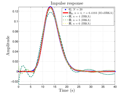
Figure 2: Impulse response of the original model $\mathbf{H}$ of order $N=20$ (solid dotted blue line), the input-delay $\mathcal{H}_{2}$-optimal model $\hat{\mathbf{H}}_{d}$ of order $n=4$ (solid red line) and the delay-free $\mathcal{H}_{2}$-optimal models $\hat{\mathbf{H}}$ of order $n=\{4,5,6\}$ (dashed dark green, light green and yellow lines).

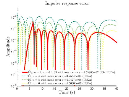
Figure 3: Impulse response error between the original model $\mathbf{H}$ of order $N=20$ and the input-delay $\mathcal{H}_{2}$-optimal model $\hat{\mathbf{H}}_{d}$ of order $n=4$ (solid red line) and the delay-free $\mathcal{H}_{2}$-optimal models $\hat{\mathbf{H}}$ of order $n=\{4,5,6\}$ (dashed dark green, light green and yellow lines).

6 Conclusion

The main contribution of this paper is the derivation of the first-order $\mathcal{H}_{2}$ optimality conditions for Problem 2.1. It forms a direct extension of the bi-tangential interpolation conditions of the delay-free case derived in [1, 2]. Theorem 4.1 establishes that if $\hat{\mathbf{H}}_{d}=\hat{\boldsymbol{\Delta}}_{o}\hat{\mathbf{H}}\hat{\boldsymbol{\Delta}}_{i}$ is a local optimum, then the parameters of this latter verify an extended set of matricial equalities. These ones are of two types: first, (i) a subset of interpolation conditions (12) satisfied by the rational part $\hat{\mathbf{H}}$ of $\hat{\mathbf{H}}_{d}$, which generalizes the delay-free case; secondly, (ii) a subset of matricial relationships (13) focussing on the input/output delay blocks $\hat{\boldsymbol{\Delta}}_{o},~{}\hat{\boldsymbol{\Delta}}_{i}$. These conditions all are dependent on the reduced order model parametrization described by $\hat{\mathbf{b}}_{k},~{}\hat{\mathbf{c}}_{k},~{}\hat{\lambda}_{k},~{}\hat{\tau}_{l}$ and $\hat{\gamma}_{m}$, and solving Problem 2.1 requires to tackle a non-convex optmization problem. Nevertheless, an algorithm referred to as IO-dIRKA, has been proposed to practically address this issue. This latter decorrelates the decision variables between them by solving, firstly for given $\hat{\boldsymbol{\Delta}}_{i},~{}\hat{\boldsymbol{\Delta}}_{o}$ matrices, an optimal $\mathcal{H}_{2}$ approximation problem, and then, in a second stage, a nonlinear maximization problem (16) to determine the optimal values of the delays. Both optimizations rely on descent methods, taking benefits from the analytical expressions of the gradients of the $\mathcal{H}_{2}$ mismatch gap $\nabla\mathcal{J}$. Numerical experiment have also been presented, illustrating the benefit of the proposed approximation delay structure with respect to standard delay-free approximation methods.

References

[1]
S. Gugercin, A. C. Antoulas, C. Beattie, model reduction for
large-scale linear dynamical systems, SIAM Journal on matrix analysis and
applications 30 (2) (2008) 609–638.
[2]
P. Van Dooren, K. A. Gallivan, P.-A. Absil, -optimal model
reduction of MIMO systems, Applied Mathematics Letters 21 (12) (2008)
1267–1273.
[3]
J. T. Spanos, M. H. Milman, D. L. Mingori, A new algorithm for optimal
model reduction, Automatica 28 (5) (1992) 897–909.
[4]
D. C. Hyland, D. S. Bernstein, The optimal projection equations for model
reduction and the relationships among the methods of Wilson, Skelton, and
Moore, IEEE Transactions on Automatic Control 30 (12) (1985) 1201–1211.
[5]
D. A. Wilson, Optimum solution of model-reduction problem, in: Proceedings of
the Institution of Electrical Engineers, Vol. 117, IET, 1970, pp. 1161–1165.
[6]
L. Meier III, D. G. Luenberger, Approximation of linear constant systems, IEEE
Transactions on Automatic Control 12 (5) (1967) 585–588.
[7]
C. A. Beattie, S. Gugercin, A trust region method for optimal
model reduction, in: Proceedings of the 48th Conference on Decision and
Control, IEEE, 2009, pp. 5370–5375.
[8]
E. J. Grimme, Krylov projection methods for model reduction, Ph.D. thesis,
Ph.D. thesis, University of Illinois, Urbana-Champaign, Urbana, IL (1997).
[9]
A. Astolfi, Model reduction by moment matching for linear and nonlinear
systems, IEEE Transactions on Automatic Control 55 (10) (2010) 2321–2336.
[10]
A. C. Antoulas, D. C. Sorensen, S. Gugercin, A survey of model reduction
methods for large-scale systems, Contemporary mathematics 280 (2001)
193–220.
[11]
A. C. Antoulas, Approximation of large-scale dynamical systems, Vol. 6, SIAM,
2005.
[12]
M. Opmeer, Optimal model reduction for non-rational functions, in: 14th annual
European Control Conference July 15th, Vol. to appear, 2015.
[13]
Y. Halevi, Reduced-order models with delay, International journal of control
64 (4) (1996) 733–744.
[14]
G. Scarciotti, A. Astolfi, Model reduction by moment matching for linear
time-delay systems, in: 19th IFAC World Congress, Cape Town, South Africa,
August 24, Vol. 29, 2014.
[15]
I. Pontes Duff, C. Poussot-Vassal, C. Seren, Realization independent single
time-delay dynamical model interpolation and -optimal
approximation, in: Proceedings of the 54st IEEE Conference on Decision and
Control, 2015.
[16]
P. Schulze, B. Unger, Data-driven interpolation of dynamical systems with
delay, Preprint-Reihe des Instituts fur Mathematik, Technische Universitat
Berlin.
[17]
A. J. Mayo, A. C. Antoulas, A framework for the solution of the generalized
realization problem, Linear algebra and its applications 425 (2) (2007)
634–662.
[18]
C. Poussot-Vassal, P. Vuillemin, Introduction to MORE: a MOdel REduction
Toolbox, in: Proceedings of the IEEE Multi-conference on Systems and
Control, Dubrovnik, Croatia, 2012, pp. 776–781.