Negative pressure in shear thickening bands of a dilatant fluid

Abstract

We perform experiments and numerical simulations to investigate spatial distribution of pressure in a sheared dilatant fluid of the Taylor-Couette flow under a constant external shear stress. In a certain range of shear stress, the flow undergoes the shear thickening oscillation around 20 Hz. We find that, during the oscillation, a localized thickened band rotates around the axis with the flow. Based upon experiments and numerical simulations, we show that a major part of the thickened band is under negative pressure even in the case of discontinuous shear thickening, which indicates that the thickening is caused by Reynolds dilatancy; the dilatancy causes the negative pressure in interstitial fluid, which generates contact structure in the granular medium., then frictional resistance hinders rearrangement of the structure and solidifies the medium.

I Introduction

A fluid with suspended particles have an apparent viscosity different from that of the medium fluid. If the total volume of particles is much smaller than that of fluid, the suspension behaves as a Newtonian fluid with the viscosity given by well known Einstein’s viscosity formula Landau and Lifshitz (1987). In the case of high volume fraction, the fluid exhibits non-Newtonian behaviors. The viscosity decreases with increasing shear rate (shear thinning)Rutgers (1962) in many materials such as mud, paint, and ketchup. Shear thickening behaviors, i.e., increasing viscosity with shear rate, are also observed in some other suspensions. In the extreme case such as the dense suspension of starch particles in water, the fluid almost solidifies under shear stress; the viscosity increases discontinuously by orders of magnitude Wagner and Brady (2009); Fall et al. (2008); Brown and Jaeger (2009). They are often called “dilatant fluid” due to apparent analogy to Reynolds dilatancy of granular media Freundlich and Juliusburger (1935), and their fascinating and unintuitive behaviors are popular subjects for science demonstrations Merkt et al. (2004); Ebata et al. (2009); von Kann et al. (2013); Isa et al. (2009); Nagahiro et al. (2013).

The mechanism of discontinuous shear thickening (DST) is still under debate. A promising explanation is related to the dilatancy and jamming Cates et al. (2005). As stated in the Reynolds principle of dilatancy, dense granular media must dilate when they deform. If a suspension is confined, the dilation leads to jamming and then shear stress abruptly increases. It is numerically Otsuki and Hayakawa (2011) and experimentally Bi et al. (2011) demonstrated that contact friction between particles is important for DST in a shear flow of dry granular systems. The frictional contacts is found to be essential for DST also for the hard-sphere suspensions Seto et al. (2013); Mari et al. (2014); Fernandez et al. (2013). Lin et al. recently found that even in continuous shear thickening the contact forces between particles dominate hydrodynamic interactions Lin et al. (2015). With these results, it is argued that DST is a consequence of jamming caused by dilatancy in a medium of frictional particles.

It has been known that the uniform steady shear flow is unstable for shear thickening media and noisy fluctuation or periodic oscillation under a constant external shear stress have been reported Laun et al. (1991); Lootens et al. (2005); Nagahiro et al. (2013); Larsen et al. (2014). Such oscillation is a general feature of a shear thickening fluid with the S-shaped flow curve Bashkirtseva et al. (2010), and may be interpreted as shear thickening oscillation, i.e., a periodic alternation between the thickened and thinned state of the media under a constant external stress that is in the unstable branch of the flow curve. This oscillation has been predicted by a fluid dynamics model for shear thickening media Nakanishi and Mitarai (2011); Nakanishi et al. (2012), and observed experimentally in shear flows of macroscopic width of several centimeters Nagahiro et al. (2013). The frequency of the oscillation is expected to depend weakly on the width of the flow if one assume spatially uniform thickening, but spatial inhomogeneity develops quickly and usually only one thickened band remains after initial transient. Even with such spatial inhomogeneity, a clear oscillation around 20 Hz appears in the experiment with a macroscopic flow width around 5 cm, and its frequency hardly depends on either the flow width or the external stress Nagahiro et al. (2013). There are also experiments that report similar oscillations in the shear flows with narrower width, typically 1 mm or less than a hundred of particle diametersLaun et al. (1991); Lootens et al. (2005); Larsen et al. (2014), in which case the particle discreteness may play some role.

In this work, we investigate the Taylor-Couette flow of a dilatant fluid by experiments and numerical simulations. We measure the off-center force on the axis and the local pressure at the wall of the outer cylinder. We also perform numerical simulations for a three dimensional system using a fluid dynamics model developed by the authors Nakanishi and Mitarai (2011); Nakanishi et al. (2012). The comparison of the simulation results with the experimental data reveal the spatial distribution of pressure and viscosity in the flow. We find that the thickening region strongly localizes, and forms two types of thickening bands, which distinctly have positive and negative pressure. It is remarkable that, even in the DST regime, the dominant thickening bands extend in the stretching direction under negative pressure, namely, the system jams due to tensile stress. Our local pressure measurement uncovers that the negative pressure is limited by the Laplace pressure, suggesting that the jamming under the tensile stress is sustained by the interstitial fluid.

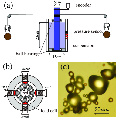
Figure 1: (a) Schematic illustration of the experimental setup. A cylindrical container with a rotatable center rod is filled with starch-water mixture. A pair of weights are hung through steel wires wound around the center rod to give constant torque to the rod in CCW direction. The flow width $h$, i.e. the gap between the cylinder and the rod, is $5$ cm. (b) Top view of the upper fixed end of the center rod. The ball bearing is supported at four points by load cells to measure the force acting on the rod. (c) Micrograph of the potato-starch particles.

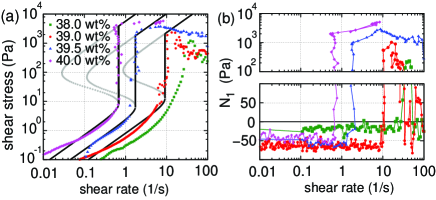
Figure 2: Flow curves (a) and the first normal stress difference $N_{1}$ (b) of the potatostarch suspension density-matched by CeCl. The data are obtained by a cone-plate rheometer (Haake Mars) with the cone angle 82^∘, the gap size 140 $\mu$m, and the cone diameter 35 mm. The data beyond DST are not meaningful because samples are fractured upon solidification. The solid curves are those for the model used in the simulations (Sec. III.1).

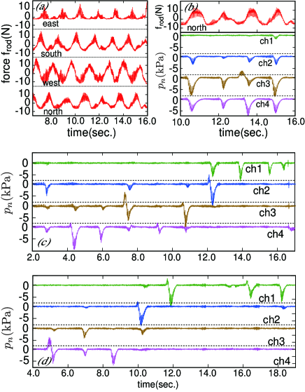
Figure 3: Time evolutions of the off-center force on the center rod and the normal pressure at the wall of the outer cylinder. The hydrostatic pressure is subtracted from the normal pressures. (a) Off-center forces for $S_{e}=1.46$ kPa. (b) The off-center force on the north load cell and the normal pressures for $S_{e}=1.46$ kPa plotted with the common time axis. (c,d) Normal pressures for $S_{e}=0.84$ kPa and for $S_{e}=1.26$ kPa. The suspension is a 39 wt$\%$ mixture of potato starch and an aqueous solution of CsCl with a density of 1.75 ${\rm g/cm^{3}}$.

II Experiment

II.1 Systems

Our experimental setup is shown in Fig.1(a). The container consists of an acrylic outer cylinder (15 cm inner diameter) and an acrylic center rod (5 cm diameter) with an aluminum base plate and a lid; the gap $h$ between the outer cylinder and the central rod is $h=5$ cm. The fluid fills the container up to $\ell=23\,{\rm cm}$ from the bottom with its surface open to the air. The center rod is supported with a couple of ball bearings: one embedded in the base plate and the other in the lid of the container. Constant torque in the counterclockwise(CCW) direction is applied on the center rod by a pair of weights on the opposite sides through steel wires wound around the rod. The weights are hung through spring-dumper systems to reduce the vibration transmitted from the rod. The both weights are the same so that no net force should be applied on the rod. We use the weights in the range of $0.20\sim 4.0{0}\;{\rm kg}$, which corresponds to the external shear stress $S_{e}=0.08\sim 1.68\;{\rm kPa}$ at the rod surface. In order to enforce the no-slip condition, the surface is lined with water-proof sand paper.

The off-center force on the center rod from the suspension is measured by four load cells (Kyowa LMB-A-100N), which support the upper ball bearing at four points as shown in Fig 1(b). To measure both negative and positive force, the load cells are pressed by screws and the zero-point of the load cells is set when the rod is stationary before each experiment. We label them as “north”, “south”, “east” and “west” by their directions. Note that precise calibration in the off-center force measurements is difficult due to the friction at the contacts between a load cell and the ball bearing.

We also measure the normal pressure $p_{n}$ at the surface of the outer cylinder by four pressure sensors (Kyowa PGM-G-02KG). They are located to the “north” of the center and aligned along the axial direction at intervals of 2 cm with the shallowest one located at 7.5 cm below the fluid surface; they are labelled as “ch1”, “ch2”, “ch3” and “ch4” from the top to the bottom. The normal pressure obtained by these sensors is the sum of the pressures by both the interstitial liquid and the particles.

We use the potatostarch particles (Hokuren) of irregular shape with their sizes distributed over the range of $5\sim 30\,{\rm\mu m}$ [Fig.1(c)]. The powder is dried for 24 hours at $60^{\circ}\rm C$ and 35$\%$ humidity, and then the water-starch mixture is prepared with the density matched aqueous solution ($\rho=1.75\,{\rm g/cm^{3}}$) of cesium chloride (CsCl).

II.2 Results

Rheology of the media:

First of all, the flow curves and the normal stress difference $N_{1}$ measured by a cone-plate rheometer for the water-starch mixtures are shown in Fig.2 to present rheological properties of the media that we are going to study. DST is clearly observed except for the 38 wt% mixture. The data presented in the rest of this report are for the 39 wt% mixture. In our experimental setup of Fig.1(a), the shear thickening oscillation of 20 Hz is observed for $S_{e}\gtrsim 0.1$ kPa, as will be presented below. This is in the unstable branch of the flow curve in Fig.2(a), thus is consistent with our interpretation that the 20 Hz oscillation is the shear thickening oscillation. The solid curves and gray plots in Fig.2(a) are the flow curves upon increasing shear rate and the unstable branch, respectively, by the model used in the simulations with the parameters listed in Table 1. One can see that the rheology of the media is well reproduced by the model. Detailed description of the model is given in Sec.IIIA. The normal stress difference $N_{1}$ shown in Fig.2(b) are negative for small shear rate, but upon DST they jump to large positive values in agreement with previous resultsRoyer et al. (2016).

Measurement by Taylor-Couette cell:

Figure 3 shows the typical time developments of the off-center force $f_{\rm rod}$ on the center rod and the normal pressure $p_{n}$ at the outer cylinder during the shear thickening oscillation. In Fig.3(a), the results from the four load cells at east, south, west, and north are shown for $S_{e}=1.46$ kPa. The curves are roughly sinusoidal shape with the period $\tau_{b}\simeq 1.4$ s overlaid by the characteristic oscillation of shear thickening with the period $\tau_{\rm sto}\simeq 0.05$ s. The time shifts between the plots for the neighboring load cells are $1/4$ of their periods, indicating that the direction of the off-center force rotates with the flow to the CCW direction.

Figure 3(b) shows the temporal variations of the off-center force $f_{\rm rod}$ on the north load cell along with the normal pressures $p_{n}$ measured by the four pressure sensors on the outer cylinder wall in the north. Note that the hydrostatic pressure is subtracted from the normal pressures. We observe periodic negative pulses in $p_{n}$ with the width $\tau_{p}\simeq 0.6$ s. They are slightly ahead of the peaks in the “north” component of $f_{\rm rod}$. One may notice that the negative pulses are occasionally preceded by relatively weak positive pulses. It is also notable that many of the pulses are detected only by a couple of sensors, which reveals that the pressure fluctuation is localized in a region of a few centimeters thickness in the axial direction. These features are also seen in the $p_{n}$ data for $S_{e}=$1.05 and 0.84 kPa in Fig.3(c,d).

Figure 4: Normalized rank plots, i.e. the integrated distributions, of the peak values of the normal pressure $p_{n}$ for the negative pulses (left panels) and the positive pulses (right panels) for various external shear stresses $S_{e}$. The data ranks are plotted against the bare peak values in the upper plots while the peak values are scaled by the external stress $S_{e}$ in the lower plots. The plots for the various $S_{e}$ overlap with each other better in the bare plots for the negative pulse while data scatter is smaller in the scaled plots for the positive pulse.

Positive and negative pressure pulses:

Figure 4 shows the integrated distributions of the peak values of $p_{n}$ for the positive and the negative pressure pulses for various external shear stresses. The integrated distributions are plotted against the peak values in the upper panels, while the horizontal axes are scaled with the external shear stresses $S_{e}$ in the lower panels. For the negative pulse, the plots in the upper panel collapse along a single common curve better than those in the lower panel. As for the positive pulse, better collapse is obtained by the scaled plots in the lower panel.

The better collapse for the scaled data of the positive pulse means that the pressure in the positive pulse is proportional to the externally applied shear stress. This result may corresponds to the linear correlation between the first normal stress difference $N_{1}$ and external shear stress reported by Lootens et. al Lootens et al. (2005), and in accords with the picture of the jamming mechanism.

In contrast to the positive pulse, the peak pressure distribution of the negative pulse is almost independent of $S_{e}$, and the maximum negative pressure in the distributions are $-14\sim-10$ kPa. These values are close to the Laplace pressure $-2\gamma/R$, which gives $-10\,{\rm kPa}$ for the average particle size of our potatostarch particles ($15\,{\rm\mu m}$) and the surface tension of water ($73$ mN/m).

Figure 5: Snapshots of the numerical simulation of Taylor-Couette flow from the uniformly relaxed initial state by a phenomenological fluid dynamics model of a dilatant fluid Nakanishi and Mitarai (2011); Nakanishi et al. (2012). The depth of the flow is $\ell=2.6$, the gap between the two cylinders is $h=1.5$, and the external stress on the surface of center rod is $S_{e}=1.5$. The arrow indicates the direction of rotation. (a) Isosurface of viscosity for $\eta=2$. (b) Isosurface of isotropic pressure for $p=1$ (red) and $p=-1$ (blue). The unit system is defined in the text.

III Numerical Simulation

III.1 Model

We performed three-dimensional (3-$d$) simulations for the Taylor-Couette flow using a fluid dynamic model of a dilatant fluid Nakanishi and Mitarai (2011); Nakanishi et al. (2012). The model is based on the incompressible Navier-Stokes equation

$$\rho{Dv_{i}\over Dt} ={\partial\over\partial x_{j}}\big{(}-p\delta_{i,j}+\sigma_{i,j}\big{)}$$ (1)

with the stress and the strain rate tensors

$$\sigma_{i,j} =\eta(\phi)\dot{\gamma}_{i,j},$$ (2)

$$\dot{\gamma}_{i,j} \equiv{\partial v_{i}\over\partial x_{j}}+{\partial v_{j}\over\partial x_{i}},$$ (3)

where Lagrange derivative is denoted by

$${D\;\over Dt}\equiv{\partial\;\over\partial t}+v_{i}{\partial\;\over\partial x_{i}},$$

and Einstein rule for the summation is employed. The scalar field $\phi$ is a phenomenological parameter supposed to represent the internal structure of the medium, such as the contact number of grains, but not a conserved quantity like the volume fraction. The pressure $p$ is determined by the incompressible condition

$${\partial v_{i}\over\partial x_{i}}=0.$$ (4)

The viscosity of the medium $\eta$ is a function of $\phi$, and local value of $\phi(\bm{r})$ is driven by the shear deformation to the value $\phi_{*}$ determined by the local shear stress $S$ of the medium,

$$r{D\phi(\bm{r})\over Dt} =-\dot{\gamma}\big{(}\phi(\bm{r})-\phi_{*}(S)\big{)},$$ (5)

where $r$ is a dimensionless parameter and

$$\dot{\gamma}^{2} \equiv{1\over 2}\dot{\gamma}_{i,j}\dot{\gamma}_{j,i},$$ (6)

$$S^{2} \equiv{1\over 2}\sigma_{i,j}\sigma_{j,i}.$$ (7)

Note that in Eq.(5) the time derivative is assumed to be proportional to the strain rate, which means that the change of $\phi$ is driven by the strain and the dimensionless parameter $r$ represents the strain scale that drives $\phi$. We also like to remark that our model is not for the shear rate thickening, but for the shear stress thickening because the viscosity is determined by the shear stress $S$ through the function $\phi_{*}(S)$.

concentration [wt%] $\phi_{M}$ $S_{0}$ [Pa] $\eta_{0}$ [Pa$\cdot$s] $A$ $\tau_{0}$ [s] $\ell_{0}$ [cm] 40.0 0.87 10.0 7.0 1 0.7 5.3 39.5 0.86 8.0 2.2 1 0.28 1.9 39.0 0.85 15.0 0.8 1 0.53 0.49

Table 1: Parameters used for the plots (solid and dotted lines) by the model in Fig.2. The values for $\tau_{0}$ and $\ell_{0}$ are estimated for $\rho=1.75\times 10^{3}{\rm kg/m^{3}}$.

The functional forms of $\phi_{*}(S)$ and $\eta(\phi)$ are chosen so that the model can simulate behaviors of the dilatant fluid. Employing simple functional forms

$$\phi_{*}(S) \equiv\phi_{M}{(S/S_{0})^{2}\over 1+(S/S_{0})^{2}},$$ (8)

$$\eta(\phi) \equiv\eta_{0}\exp\left[A{\phi\over 1-\phi}\right],$$ (9)

we have demonstrated that the model reproduces most of the characteristic behaviors of the dilatant fluidsNakanishi and Mitarai (2011); Nakanishi et al. (2012); Nagahiro et al. (2013).

Assuming the steady uniform shear flow under an external shear stress $S$, the shear rate $\dot{\gamma}$ is given by

$$\dot{\gamma}={S\over\eta\left[\phi_{*}(S)\right]}.$$ (10)

This gives the S-shaped flow curve, which have the unstable branch between the low and the high stress stable branches. In Fig.2, this relation is compared with the experimental flow curves obtained by increasing stress. The solid curves for the model are drawn by assuming that the stress jump from the low stress branch to the high stress branch at the end of the low stress branch. The model parameters used in Fig.2 are listed in Table 1.

In this model, the system is characterized by the dimensional material parameters, $\rho$, $S_{0}$, $\eta_{0}$, and the dimensionless model parameters, $\phi_{M}$, $r$, $A$. As for the dimensional parameters, we can define the unit system where $\eta_{0}=S_{0}=\rho=1$, then, the time, length, and mass are measured by the units

$$\tau_{0}\equiv{\eta_{0}\over S_{0}},\quad\ell_{0}\equiv\sqrt{{\eta_{0}\over\rho}\tau_{0}},\quad m_{0}\equiv\rho\ell_{0}^{3},$$ (11)

respectively. As for the dimensionless model parameters, we took

$$\phi_{M}=0.85,\quad r=0.1,\quad A=1$$

in the 3-$d$ simulations. The time and the length units given by Eq.(11) are listed also in Table 1 for the present system with $\rho=1.75\times 10^{3}{\rm kg/m^{3}}$.

We have already demonstrated that the model reproduces basic properties of a dilatant fluids such as DST, the hysteresis upon changing shear rate, or instantaneous solidification by an external impactNakanishi and Mitarai (2011). The shear thickening oscillation had been predicted by this model and was experimentally observed as had been predictedNagahiro et al. (2013).

We employ the Highly Simplified Marker and Cell (HSMAC) algorithmHirt and Cook (1972) for numerical simulations. As for the boundary conditions at the cylinder and the rod surfaces, we emulate the ones in our experiment, i.e. the no-slip fixed boundary at the outer cylinder and the no-slip boundary with the rotating center rod, which rotates so as to give an average shear stress on the surface equal to the applied shear stress $S_{e}$; we ignore the mass of the rod. As for the boundaries in the rotating axis direction, however, we employ the periodic boundary condition for simplicity. We set diameter of the center rod $d=2$, the flow width $h=1.5$ and the fluid depth $\ell=2.6$ by the units (11). With the parameters for the present medium, they are comparable with the ones for our experimental set up.

III.2 Results

A uniform steady flow is unstable for the external stress $S_{e}$ beyond a certain value. Figure 5 show the system evolution during the first 2.5 rotations of the central rod under the external stress $S_{e}=1.5$, which is in the unstable regime. The system is initially in the uniform relaxed state. The upper panels show the isosurfaces at $\eta=2$ (green) and the lower panels show those for the isotropic pressure $p=+1$ (red) and for $p=-1$ (blue). The results show that the viscosity and pressure distribution are not cylindrically symmetric. High viscosity regions initially appear near the center rod ($t\lesssim 3.6$), then gradually merge into a few flat regions ($t\lesssim 21.2$), and eventually form a single fan-shape thickening band, in which positive and negative pressure segments extend in different directions ($t=66.4$), i.e. the compressing and the stretching directions in the shear flow caused by the rotating center rod. The thickening band with the positive and negative segments rotates slowly with the center rod. As a result, the positive pressure segments always go ahead of the negative pressure segments at the surface of the outer cylinder. This is in agreement with the results of our normal pressure measurement, where the positive pulses precede the negative pulses.

In the simulations, the localized thickening band shows the shear thickening oscillation whose period is much faster than that of the rotation. This oscillation in the simulation should correspond with the 20 Hz oscillation in our observation. The basic mechanism of the oscillation is the same with that in the 2-$d$ simple shear flowNakanishi et al. (2012); in the S-shaped flow curve, there exists a range of the shear stress where the steady flow is unstable; under an external shear stress in the unstable range, no steady shear flow is possible and the system oscillates between the thickened and the relaxed states. In the shear stress thickening, the spatially uniform flow in the directions perpendicular to the shearing is intrinsically unstable because localized thickened bands can take most of the external stress, leaving the rest of the medium in the unthickened state under low stress.

By the simulations of the Taylor-Couette flow, we can observe the dynamics of the thickened band; starting from the uniform relaxed state, the thickening regions first appear in the initial transient time near the inner rod, where the shear rate is large. Then, some of the regions extend outwards, but eventually only one of them remains and reaches the outer cylinder. When the band reaches the outer cylinder, the flow decelerates. Then, it starts flowing again because the external stress is not large enough to keep the whole band in the thickened state. As the system starts flowing, the thickened band breaks in the outer regions, then the flow accelerates further until the shear stress causes thickening in the broken part of the band. During the oscillation cycle, only a part of thickening band disappears, but the rest remains thickened.

IV Discussions

The results of our numerical simulations and experiments are consistent and show that the thickening band distinctly has two types of segments: the positive pressure segment extending along the compressive direction of the shear flow and the negative pressure segment along the tensile direction. The remarkable finding is that the negative pressure segment of the shear thickening domain is dominant in volume when the medium exhibits the shear thickening oscillation in the Taylor-Couette flow.

The pressure observed by the sensors is the total pressure from both the fluid and the particles, but it should be noted that the negative contribution to the pressure only comes from the fluid because the particles cannot exert tensile force on the sensors. This may entail to the observed differences in the external shear stress dependence of the pressure in the regions of positive and negative pressure as shown in Fig. 4; the pressure in the positive domains increases linearly with the external shear stress $S_{e}$, while the negative pressure does not seem to depend on $S_{e}$, but remains below the Laplace pressure. Such linear dependence of the positive pressure has been reported also in Ref.Lootens et al. (2005), and suggests that the positive pressure is dominated by the particle pressure, that propagates along force chains in the jammed granular medium. As for the negative pressure, it should be caused by the fluid in the interstitial space that tends to expand upon deformation of the medium due to Reynolds dilatancy. In the experiment, thickening band does not reach to the fluid-air interface at the top. Therefore, the fact that the negative pressure is limited by the Laplace pressure indicates that there exist the fluid-air interfaces possibly at the surface of micro-bubbles in the medium.

The shear thickening due to jamming in the negative pressure region has not been discussed in the literature, but it is natural for the granular medium with friction because the negative pressure in the interstitial fluid should increase contacts among the granular particles and the friction resists against rearrangement of the contact structure in the medium. It should be also noted that the shear thickening in the tensile deformation is easily observed in a simple demonstration by just pouring the starch-water mixture out of a cup, and the effect of shear thickening on drop formation in a granular suspension has been studiedPan et al. (2015).

Although our experiments clearly show the existence of the negative pressure regions, it has not been reported in the literature ; some experiments report only positive pressure when DST occursFall et al. (2008); Lootens et al. (2005); Brown and Jaeger (2012). These experiments, however, do not observe the spatial variation of the pressure, but measure only total force on the upper plate of a cone-plate or plate-plate type rheometer, using small samples. In such measurement, the effect of the negative pressure may be hidden by the large positive pressure under strong external shear stress in the case where the value of the negative pressure is limited, even though the size of the negative pressure region is not small in comparison with that of the positive pressure.

In conclusion, our experiments and numerical simulations show that, the negative pressure segment along the tensile direction is dominant in the shear thickening band of a dilatant fluid. The negative pressure in the thickening bands indicates that the thickening is caused by Reynolds dilatancy; the negative pressure caused by the dilatancy generates contact structure in the granular medium, and the solidification of the medium is due to the frictional resistance against the rearrangement of the structure.