Lattice QCD studies on baryon interactions
from Lüscher’s finite volume method
and HAL QCD method

Abstract:

A comparative study between the Lüscher’s finite volume method and the time-dependent HAL QCD method is given for the $\Xi\Xi$(${}^{1}\mathrm{S}_{0}$) interaction as an illustrative example. By employing the smeared source and the wall source for the interpolating operators, we show that the effective energy shifts $\Delta E_{\rm eff}(t)$ in Lüscher’s method do not agree between different sources, yet both exhibit fake plateaux. On the other hand, the interaction kernels $V(\vec{r})$ obtained from the two sources in the HAL QCD method agree with each other already for modest values of $t$. We show that the energy eigenvalues $\Delta E(L)$ in finite lattice volumes ($L^{3}$) calculated by $V(\vec{r})$ indicate that there is no bound state in the $\Xi\Xi(^{1}\mathrm{S}_{0})$ channel at $m_{\pi}=0.51$ GeV in 2+1 flavor QCD.

1 Introduction

To investigate the hadron-hadron interactions, two methods have been proposed so far; the Lüscher’s finite volume method [1] and the HAL QCD method [2]. In the former method, the energy shift of the two-body system in finite lattice box(es) is measured. It is then translated into the scattering phase shift and the binding energy in the infinite volume through the Lüscher’s formula (see e.g. a review, [3]). On the other hand, in the latter method, the interaction kernel (the non-local potential) between hadrons is first calculated in finite lattice box(es). It is then utilized to calculate the observables in the infinite volume (see the review, [4].)

For the simple example such as the $I=2$ $\pi\pi$ scattering with the heavy pion mass, a quantitative agreement of the phase shifts and the scattering lengths between the two methods has been established [5]. On the other hand, no systematic comparison between two methods for multi-baryon systems has been made so far. The purpose of the present report is to make such a comparison in the two-baryon system on the common gauge configurations. As shown below, our results indicate that an extreme care is necessary for the Lüscher’s method when it is applied to baryon-baryon interactions.

2 Lattice Setup

We use 2+1 flavor QCD gauge configurations generated with the Iwasaki gauge action and the nonperturbatively ${\cal O}(a)$-improved Wilson quark action at $\beta=1.90$ and $c_{sw}=1.715$, which corresponds to $a^{-1}=2.194(10)$ GeV, $m_{\pi}=0.51$ GeV, $m_{N}=1.32$ GeV, and $m_{\Xi}=1.46$ GeV [6]. We take the three lattice volumes, $L^{3}\times T$ = $40^{3}\times 48$, $48^{3}\times 48$ and $64^{3}\times 64$, which correspond to the spatial sizes 3.6 fm, 4.3 fm and 5.8 fm, respectively. These configurations are exactly the same as those used by Yamazaki et al. for nucleon-nucleon (NN) systems [6]. In order to improve the statistics, we make a use of the rotation symmetry for $48^{3}\times 48$ and $64^{3}\times 64$ lattices.

In this report, we focus on the baryon-baryon interaction in the $\Xi\Xi(^{1}\mathrm{S}_{0})$ channel instead of the NN channel. This is because the statistical error in the hyperon system is much smaller than those of the nucleon system due to the strange quark mass, so that the quantitative comparison between the two methods can be made clearer. Also, the $\Xi\Xi(^{1}\mathrm{S}_{0})$ channel belongs to the same SU(3) flavor multiplet (the 27 representation) as the NN$(^{1}\mathrm{S}_{0})$, so the characteristic features of the interaction are expected to be similar. We employ interpolating operators for $\Xi$ as

$$\Xi_{0}^{\alpha}=\varepsilon^{abc}(s_{a}C\gamma_{5}u_{b})s_{c}^{\alpha},\quad\Xi_{-}^{\alpha}=\varepsilon^{abc}(s_{a}C\gamma_{5}d_{b})s_{c}^{\alpha}$$ (1)

with relativistic (4-spinor) quark fields and $C=\gamma_{4}\gamma_{2}$. The quark propagator is solved with the periodic boundary condition in all directions.

With Coulomb gauge fixing, we employ both smeared source and wall source for the interpolating operators to check whether observables are independent of the choice. As for the wall source, we adopt $q^{\mathrm{wall}}(t_{0})=\sum_{\vec{x}}q(\vec{x},t_{0})$, while for the smeared source, we take the exponentially smeared quark, $q^{\mathrm{smear}}(\vec{x},t_{0})=\sum_{\vec{y}}f(|\vec{x}-\vec{y}|)q(\vec{y},t_{0})$ where $f(r\neq 0)=Ae^{-Br}$ and $f(r=0)=1$ with coefficients $A$, $B$ taken from [6], so that the smeared source is exactly the same as [6]. Our lattice parameters are summarized in Table 1. For the smeared source, (# conf. $\times$ # sources) in Yamazaki et al.  [6] is (200 $\times$ 192), (200 $\times$ 192) and (190 $\times$ 256) for $L^{3}=40^{3}$, $48^{3}$ and $64^{3}$, respectively, and the ratio of the statistics in this work to Yamazaki et al. is about 1.0, 5.3 and 0.32 for each $L$.

volume	# conf.	# smeared source	parameter $(A,B)$	# wall source
$40^{3}\times 48$	$200$	$192$	$(0.8,0.22)$	$48$
$48^{3}\times 48$	$200$	$4\times 256$	$(0.8,0.23)$	$4\times 48$
$64^{3}\times 64$	$327$	$1\times 48$	$(0.8,0.23)$	$4\times 32$

Table 1: Lattice QCD setup. For some of the # source, an extra factor 4 from rotations is presented.

3 Lüscher’s Finite Volume Method

3.1 Effective energy shift

In the Lüscher’s method, the key quantity is the energy shift of the two-body system in the finite volume, $\Delta E(L)=E^{BB}-2m^{B}$, where $E^{BB}$ is the ground state energy of the two baryons and $m^{B}$ is the mass of a single baryon. The Lüscher’s formula relates $k$ of $\Delta E(L)=2\sqrt{(m^{B})^{2}+k^{2}}-2m^{B}$ to the phase shift $\delta(k)$ in the infinite volume as [1]

$$k\cot\delta(k)=\frac{1}{\pi L}\sum_{\vec{n}\in\mathbf{Z}^{3}}\frac{1}{|\vec{n}|^{2}-|\frac{\vec{k}L}{2\pi}|^{2}}.$$ (2)

In practice, $\Delta E(L)$ is often obtained from the plateau of the effective energy shift $\Delta E_{\mathrm{eff}}(t)$ at large $t$ [6],

$$\Delta E_{\mathrm{eff}}(t)=E_{\mathrm{eff}}^{BB}(t)-2m_{\mathrm{eff}}^{B}(t),$$ (3)

where $m_{\mathrm{eff}}^{B}(t)=\ln(G^{B}(t)/G^{B}(t+1))$ and $E_{\mathrm{eff}}^{BB}(t)=\ln(G^{BB}(t)/G^{BB}(t+1))$ with $G^{B}(t)$ and $G^{BB}(t)$ being the correlation functions of a single baryon and two baryons, respectively. An advantage of taking the difference $\Delta E_{\mathrm{eff}}(t)$ is that a correlation between $G^{B}(t)$ and $G^{BB}(t)$ on each configuration makes the absolute magnitude of the statistical error for $\Delta E_{\mathrm{eff}}(t)$ much smaller than that for $G^{BB}(t)$. In addition, the contaminations from single-baryon excited states at small $t$ in $\Delta E_{\mathrm{eff}}(t)$ is expected to be cancelled in part between $E_{\mathrm{eff}}^{BB}(t)$ and $2m_{\mathrm{eff}}^{B}(t)$. On the other hand, the contaminations from the elastic $BB$ scattering states other than the ground state appear only in $E_{\mathrm{eff}}^{BB}(t)$ and therefore they propagate into $\Delta E_{\mathrm{eff}}(t)$. Furthermore, such contaminations on a large lattice box survive even at large $t$. For example, the first excited state of the elastic $\Xi\Xi$ scattering has only $\sim 30$ MeV excitation energy in $L^{3}=64^{3}$ in the present setup: Such an excited state can be isolated only for $t\gg(30\ \mathrm{MeV})^{-1}\sim\mathcal{O}(10)$ fm. This consideration indicates that fitting a plateau-like structure of $\Delta E_{\mathrm{eff}}(t)$ for moderate values of $t$ is dangerous to extract the true signal in the Lüscher’s method. Indeed, in the next subsection, we demonstrate explicitly that such a fake plateau appears.

3.2 Source operator dependence

One of the useful methods to identify the fake plateau is to examine the source operator dependence of the effective energy shift. Shown in Figure 1 is $\Delta E_{\mathrm{eff}}(t)$ on a $48^{3}\times 48$ lattice for the smeared source (blue) and the wall source (red). We find plateau-like structures for both sources in the range $t=12-16$. Their magnitudes, however, do not agree with each other within statistical errors. This casts a strong doubt on the validity of plateaux in Figure 1: Either one of the plateaux (or both) is fake and the real plateau would appear for much larger $t$ where higher statistics are required to extract a few to $\sim$ 10 MeV energy shift. This analysis suggests that rather strong binding of the two-baryon systems, claimed in Refs. [6, 7] by using $\Delta E_{\mathrm{eff}}(t)$, should be taken with a grain of salt. The same caution applies also to the results of e.g. Ref.[8].

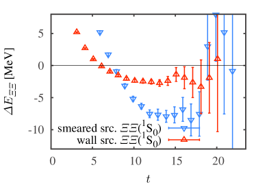
Figure 1: The effective energy shift $\Delta E_{\mathrm{eff}}(t)$ using the smeared source (blue down triangle) and the wall source (red up triangle) on a $48^{3}\times 48$ lattice. Both show plateau-like behaviors for $t=12-16$, whose values, however, are significantly different with each other.

4 HAL QCD Method

4.1 Interaction kernel

In the “time-dependent” HAL QCD method [9], we consider the Nambu-Bethe-Salpeter (NBS) correlation function $R(\vec{r},t)$;

$$R(\vec{r},t)\equiv\left\langle 0|T\{B(\vec{x}+\vec{r},t)B(\vec{x},t)\}\bar{\mathcal{J}}(0)|0\right\rangle/\left\{G^{B}(t)\right\}^{2}=\sum_{n}A_{n}\phi^{W_{n}}(\vec{r})e^{-\Delta W_{n}t}+\mathcal{O}(e^{-\Delta W_{\mathrm{th}}t}).$$ (4)

Here $B$ and $\mathcal{J}$ correspond to a sink and a source operator, respectively. The interaction energy is defined by $\Delta W_{n}=W_{n}-2m_{B}$ with $W_{n}$ being the $n$-th energy eigenvalue, while the inelastic threshold energy is defined as $\Delta W_{\mathrm{th}}=W_{\mathrm{th}}-2m_{B}$ . Below the threshold (or equivalently $t\gg(\Delta W_{\mathrm{th}})^{-1}$), the correlation $R(\vec{r},t)$ satisfies the time-dependent wave equation,

$$\left[\frac{1}{4m_{B}}\frac{\partial^{2}}{\partial t^{2}}-\frac{\partial}{\partial t}-H_{0}\right]R(\vec{r},t)=\int d\vec{r}^{\ \prime}U(\vec{r},\vec{r}^{\ \prime})R(\vec{r}^{\ \prime},t).$$ (5)

Making the velocity expansion for the non-local kernel $U(\vec{r},\vec{r}^{\ \prime})$, the leading order (LO) potential becomes

$$V(\vec{r})=\frac{1}{4m_{B}}\frac{(\partial/\partial t)^{2}R(\vec{r},t)}{R(\vec{r},t)}-\frac{(\partial/\partial t)R(\vec{r},t)}{R(\vec{r},t)}-\frac{H_{0}R(\vec{r},t)}{R(\vec{r},t)}.$$ (6)

Unlike the case of the Lüscher’s method, the time-dependent HAL QCD method does not require the ground state saturation of the two-baryon system as long as the contaminations from inelastic states in Eq. (4) are suppressed. Also, the interaction kernel (the potential) is spatially localized and is insensitive to the lattice size. This enables us to calculate the observables in the infinite volume rather easily on the basis of $V(\vec{r})$.

4.2 Source operator dependence

Let us study the source operator dependence of the potential $V(\vec{r})$ in the HAL QCD method. In Fig. 2, $R(\vec{r},t)$ with the wall source and the smeared source are shown for $t=12-15$ on a $48^{3}\times 48$ lattice. The NBS correlation functions for the smeared source are spatially localized and have a visible $t$ dependence. On the other hand, the NBS correlation functions for the wall source are spatially extended and are insensitive to $t$.

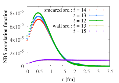
Figure 2: The NBS correlation functions for both smeared and wall sources on a $48^{3}\times 48$ lattice. The smeared source result is localized and shows strong $t$-dependence, while the wall source result is delocalized and almost $t$-independent.

Although the NBS correlation functions between different sources differ considerably, the potentials obtained from $R(\vec{r},t)$ tend to be the same [9]. Shown in Figure 3 is the central potential in the $\Xi\Xi(^{1}\mathrm{S}_{0})$ channel reconstructed from the NBS correlation function at $t=12$ for the smeared source (left) and for the wall source (right), together with its breakdown to each contribution in the right hand side of Eq. (6). For the smeared source, after sizable cancellations among different terms, the net result reaches to the red symbols. For the wall source, the cancellation is significantly milder though not negligible.

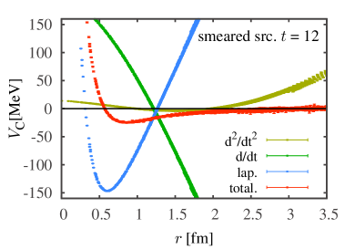
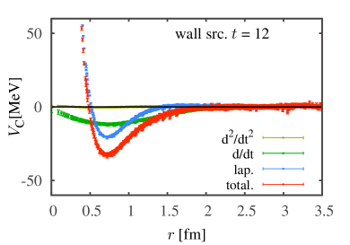
Figure 3: Breakdown of the central potential $V_{c}(r)$ in the $\Xi\Xi(^{1}\mathrm{S}_{0})$ channel on a $48^{3}\times 48$ lattice. (left) The result from the smeared source at $t=12$. (right) The result from the wall source at $t=12$.

To see the consistency of the potentials from two different sources, we show $V_{C}(r)$ at $t=12$ in Fig. 4 (left) and that at $t=15$ in Fig. 4 (right). One finds that the potential of the wall source is insensitive to the change of $t$ from 12 to 15 within statistical errors. Furthermore, as $t$ increases, the potential obtained from the smeared source approaches to that of the wall source. This tendency is also observed in other volumes.

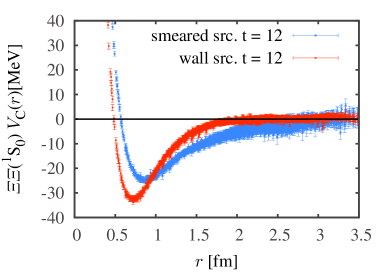
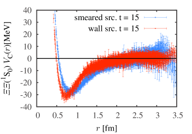
Figure 4: Comparisons of $\Xi\Xi(^{1}\mathrm{S}_{0})$ central potential by using smeared and wall sources at $t=12$ and $15$.

4.3 Energy shift from the HAL QCD method

The source independence of the potential at $t=15$ in the previous subsection gives us some confidence on its reliability in contrast to $\Delta E_{\mathrm{eff}}(t)$. We can even estimate the possible energy shift $\Delta E(L)$ in finite $L$ by using $V(\vec{r})$ [10]. Taking the potential at $t=12$ obtained by the wall source, we calculate eigenvalues of $H=H_{0}+V$ on the lattices with the spatial sizes, $L^{3}=40^{3},48^{3}$ and $64^{3}$. Resultant energy eigenvalues of the ground and first excited states are summarized in Table 2, and the lowest eigenvalues $\Delta E_{0}(L)$ are plotted as a function of $1/L^{3}$ in Fig. 5 (left). We find that $\Delta E(L)$ behaves linearly in $1/L^{3}$ and $\Delta E_{0}(L\rightarrow\infty)\rightarrow 0$. In Fig. 5 (right), we also show the phase shift from the wall source potential at $t=12$, fitted by the (two Gaussians + (Yukawa)²) [11]. Both analyses indicate that the $\Xi\Xi(^{1}\mathrm{S}_{0})$ channel at $m_{\pi}=0.51$ GeV has only scattering states in the infinite volume.

volume	$\Delta E_{0}$ [MeV]	$\Delta E_{1}$ [MeV]
$40^{3}$	$-4.55(1.18)$	$75.63(1.31)$
$48^{3}$	$-2.58(22)$	$52.87(33)$
$64^{3}$	$-1.13(9)$	$28.71(9)$

Table 2: The volume dependence of the energy eigenvalues of $H=H_{0}+V$ with the potential at $t=12$ with the wall source.

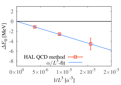
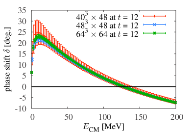
Figure 5: (left) Volume dependence of the energy eigenvalues of the ground state. (right) The phase shift of $\Xi\Xi(^{1}\mathrm{S}_{0})$ from the wall source potential, fitted by the (two Gaussian + (Yukawa)²) form [11].

5 Summary

In this report, we have examined the $\Xi\Xi(^{1}\mathrm{S}_{0})$ interaction in 2+1 flavor QCD by the Lüscher’s finite volume method and the time-dependent HAL QCD method. We have two main conclusions. First of all, the effective energy shift $\Delta E_{\mathrm{eff}}(t)$ shows plateau for $t=12-16$ both for the wall source and the smeared source, but the magnitudes of $\Delta E_{\mathrm{eff}}(t)$ do not agree with each other. This implies that either one of the plateaux (or both) is fake. Taking a specific source and extracting the energy shift at relatively small $t$ are quite dangerous even if one finds a plateau-like structure. This is because cancellations among scattering states may make a fake plateau in $\Delta E_{\mathrm{eff}}(t)$ at small $t$. A more sophisticated method such as the variational approach discussed in [10] would be necessarily for the reliable extraction of $\Delta E(L)$. Secondly, the time-dependent HAL QCD method gives a potential which is insensitive to the choice of the interpolating source operators. A tendency toward the source independence can be seen explicitly by increasing $t$. Using the potential obtained by the HAL QCD method, one can evaluate the energy eigenvalues in finite lattice boxes. The results indicate that there is no bound state in the $\Xi\Xi(^{1}\mathrm{S}_{0})$ channel at $m_{\pi}=0.51$ GeV.

References

- [1] M. Lüscher, Nucl. Phys. B 354, 531 (1991).
- [2] N. Ishii, S. Aoki and T. Hatsuda, Phys. Rev. Lett. 99 (2007) 022001 [nucl-th/0611096].
- [3] T. Yamazaki, PoS LATTICE 2014 (2015) 009 [arXiv:1503.08671 [hep-lat]], and the references therein.
- [4] S. Aoki et al. [HAL QCD Collaboration], PTEP 2012 (2012) 01A105 [arXiv:1206.5088 [hep-lat]].
- [5] T. Kurth, N. Ishii, T. Doi, S. Aoki and T. Hatsuda, JHEP 1312 (2013) 015 [arXiv:1305.4462 [hep-lat], arXiv:1305.4462].
- [6] T. Yamazaki, K. i. Ishikawa, Y. Kuramashi and A. Ukawa, Phys. Rev. D 86 (2012) 074514 [arXiv:1207.4277 [hep-lat]];
- [7] T. Yamazaki, K. i. Ishikawa, Y. Kuramashi and A. Ukawa, Phys. Rev. D 92 (2015) 1, 014501 [arXiv:1502.04182 [hep-lat]].
- [8] S. R. Beane et al. [NPLQCD Collaboration], Phys. Rev. D 85 (2012) 054511 [arXiv:1109.2889 [hep-lat]]; Phys. Rev. D 87 (2013) 3, 034506 [arXiv:1206.5219 [hep-lat]]; Phys. Rev. C 88 (2013) 2, 024003 [arXiv:1301.5790 [hep-lat]].
- [9] N. Ishii et al. [HAL QCD Collaboration], Phys. Lett. B 712 (2012) 437 [arXiv:1203.3642 [hep-lat]].
- [10] B. Charron [HAL QCD Collaboration], PoS LATTICE 2013 (2014) 223 [arXiv:1312.1032 [hep-lat]].
- [11] M. Yamada et al. [HAL QCD Collaboration], PTEP 2015 (2015) 7, 071B01 [arXiv:1503.03189 [hep-lat]].
- [12] Columbia Physics System (CPS), http://qcdoc.phys.columbia.edu/cps.html
- [13] Bridge++, http://bridge.kek.jp/Lattice-code/
- [14] M. Schröck and H. Vogt, Comput. Phys. Commun. 184 (2013) 1907 [arXiv:1212.5221 [hep-lat]].