Local Dynamics in Trained Recurrent Neural Networks

Abstract

Learning a task induces connectivity changes in neural circuits, thereby changing their dynamics. To elucidate task related neural dynamics we study trained Recurrent Neural Networks. We develop a Mean Field Theory for Reservoir Computing networks trained to have multiple fixed point attractors. Our main result is that the dynamics of the network’s output in the vicinity of attractors is governed by a low order linear Ordinary Differential Equation. Stability of the resulting ODE can be assessed, predicting training success or failure. As a consequence, networks of Rectified Linear (RLU) and of sigmoidal nonlinearities are shown to have diametrically different properties when it comes to learning attractors. Furthermore, a characteristic time constant, which remains finite at the edge of chaos, offers an explanation of the network’s output robustness in the presence of variability of the internal neural dynamics. Finally, the proposed theory predicts state dependent frequency selectivity in network response.

Task learning is considered the raison d’etre of recurrent neural networks (RNN), studied in the context of neuroscience and machine learning Mante et al. (2013); LeCun et al. (2015). Yet, theoretical understanding of trained RNN dynamics is lacking, with most of the existing physics literature addressing either random networks, designed networks (Hopfield (1982); Gardner (1988) and Ben-Yishai et al. (1995)) or designed control setting Popovych et al. (2005); Pyragas (1992); Ott et al. (1990).

In this Letter, we advance a theory of trained RNN dynamics. We consider an initially random, chaotic network whose output is trained to produce several target values, and then fed back to the network, yielding multiple fixed point attractors. This setting underlies complex tasks that were analyzed phenomenologically using rate models Mante et al. (2013); Carnevale et al. (2015); Sussillo and Barak (2013), and are the subjects of attempts Abbott et al. (2016) to extend to more realistic task performing networks Neymotin et al. (2013). Using mean field analysis, we derive the effect of training on the output dynamics in the vicinity of the training targets. Stability is then assessed, showing that training success depends on the network’s nonlinearity. Next, we show that multiple training targets can lead to state specific frequency selectivity, as observed in task adapted biological neuronal circuits Buzsaki (2006); Siegel et al. (2015). Finally, the settling time of an output of a perturbed RNN is shown to remain finite at the edge of the chaos, contrary to the varying internal state dynamics Rokni et al. (2007); Druckmann and Chklovskii (2012), for which the settling time is known to diverge Sompolinsky et al. (1988).

Model and Training Protocol

Reservoir computing Maass et al. (2002); Jaeger (2001) is a popular and simple paradigm for training RNN. A network of neurons with random recurrent connectivity (referred to as the reservoir) is equipped with readout weights trained to produce a desired output, while keeping the rest of the connectivity fixed. Such a restricted training rule implies that training affects reservoir dynamics only via feedback connections from the output Jaeger (2001); Sussillo and Abbott (2009). The dynamics (Sussillo and Abbott (2009), Sompolinsky et al. (1988); Stern et al. (2014); Rajan et al. (2010)) are given by:

$$\dot{x}=-x+Wr+w_{FB}z+w_{in}u$$ (1)

with state $x\in\mathbb{R^{\mathnormal{N}}}$ representing the synaptic input, and the firing rate given by $r(t)=\phi(x(t))$ where $\phi(x)$ is an element-wise nonlinear function of $x$, commonly set to $\phi(x)=\tanh(x)$. Output $z=w_{out}^{T}r(t)$ and input $u(t)$ are fed into the network via weight vectors $w_{FB}\text{ (resp. }w_{in})\in\mathbb{R}^{N}$ with elements i.i.d.. Elements of the connectivity matrix $W\in\mathbb{R}^{N\times N}$ are i.i.d as: $W_{ij}\mathcal{\sim N}(0,g^{2}N^{-1})$ with $g$ being a gain parameter.

The goal of the training process is to have the output $z(t)$ approximate some pre-defined target function $f(t)$. In the reservoir computing framework training is restricted to modification of the output weights $w_{out}$. Jaeger Jaeger (2001) proposed to break the readout-feedback loop, creating an auxiliary open loop system defined as:

$$\dot{x}=-x+Wr+w_{FB}f+w_{in}u$$ (2)

Here the target function $f$, rather than the readout $z$, is injected via the feedback weights $w_{FB}$. Linear regression on $r$ is used to find $w_{out}$ so that $z_{OL}=w_{out}^{T}r\approx f$.

In our case, we assume zero input ($u\equiv 0$), and target multiple fixed points of (1), corresponding to $M\ll N$ output levels $z\in\{A_{1},..A_{M}\}$ with respective solutions $\bar{x}_{1},...\bar{x}_{M}$ and rates $\bar{r}_{1}...\bar{r}_{M}$ which are obtained from the open loop system (2).

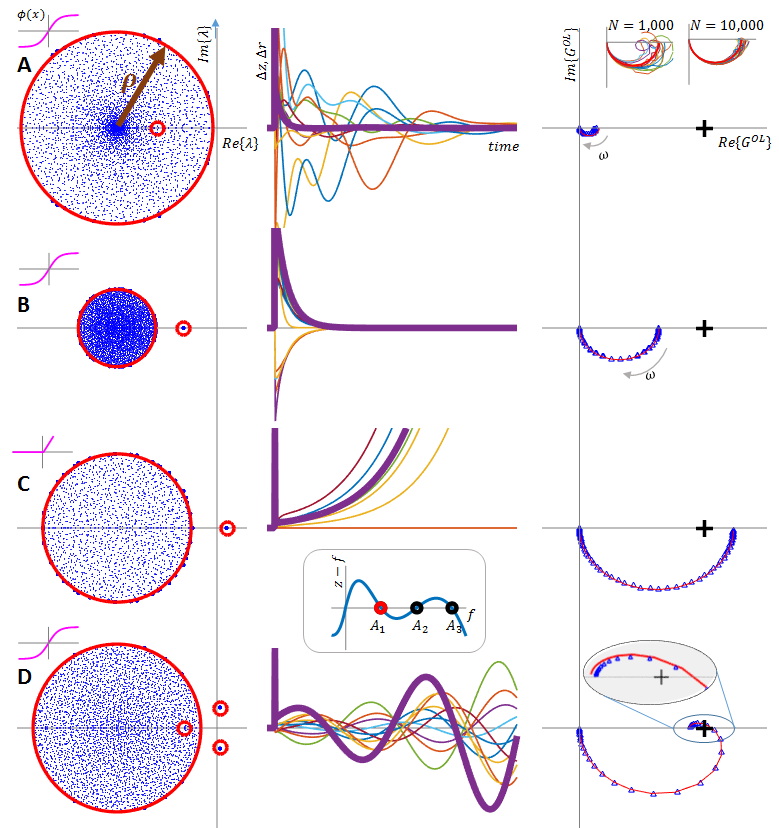
Figure 1: Analysis of a trained RNN is shown for representative cases compliant with fading memory property ($\rho<1$). A Internal dynamics are slow compared to network output ($\tau_{net}>\tau_{out}$) B Opposite case ($\tau_{net}<\tau_{out}$), here the internal state is dominated by output feedback C Unstable case ($\tau_{out}<0$) D Unstable oscillatory solution around one of the targets for $M=3$. Left: Mean field estimate (red) of closed loop spectrum compared with a finite size realization (blue dots, $N=3000$). Middle: Transient response for a $\delta-$like perturbation is shown for both output (thick line) and for 10 random neurons (thin lines). Right: MFT estimation (red) of open loop gain is compared with a finite size realization (blue). The black cross at $0+1i$ helps visualize the Nyquist criterion. Panel A inset: Finite size effects (for other cases, where $\rho$ is significantly smaller than unity finite size effects are small and not shown). Parameters: Output value was set to $A=1$ for all the cases except D where $A_{1,2,3}=\{0.5,1.0,1.5\}$ (inset), and $A_{1}$ is analysed. Nonlinearity $\phi(x)=\tanh(x)$ was used except panel C for which $\phi(x)=\max(0,x-0.1)$. The connectivity strength scale $g$ was set to 1.5, 0.5, 1.1 and 1.0 for panels A,B,C and D respectively.

Dynamics of a trained network

A necessary condition for successful training is the fading memory property Jaeger (2001) which states that the open loop system (2) must be globally asymptotically stable for the training to succeed. Remarkably, asymptotic stability can hold for suitable drive $f$ even in systems that are chaotic in the absence of external drive ($f\equiv 0$) Yildiz et al. (2012); Manjunath and Jaeger (2013). In supplemental material we show that this extended version of fading memory is necessary even for the FORCE algorithm Sussillo and Abbott (2009), known for its effectiveness for training intrinsically chaotic networks.

For a given target $f(t)\equiv A$, fading memory implies that the open loop system (2) converges to a unique stable state $\bar{x}$, given by

$$\bar{x}=W\phi(\bar{x})+w_{FB}A$$ (3)

and that the spectral radius $\rho$ of the linearized open loop dynamics $WR^{\prime}$, given by $\rho^{2}=g^{2}<r^{\prime 2}>$ Ahmadian et al. (2015); Massar and Massar (2013), is smaller than $one$. Here $R^{\prime}_{ij}=\delta_{ij}r^{\prime}_{i}$ with $r^{\prime}=\phi^{\prime}(\bar{x})=\frac{d\phi}{dx}|_{x=\bar{x}}$ is a diagonal matrix of linearized rate functions, and the average is taken over neurons.

Importantly, asymptotic stability of the open loop system (2) does not guarantee stability of the closed loop system (1). This can be understood by considering the linearization of the latter:

$$\delta\dot{x}=\left(-I+(W+w_{FB}w_{out}^{T})R^{\prime}\right)\delta x$$ (4)

For large $N$, the resulting spectrum consists of a disk-like spectral density region of radius $\rho$ associated with $WR^{\prime}$ as in the open loop system and other eigenvalues related to the feedback loop term $w_{FB}w_{out}^{T}$. We will show that exactly $M$ eigenvalues correspond to the latter and that their loci can fall either inside or outside the spectral density disk. Figure 1 shows how these loci determine stability, convergence times and oscillations for networks that comply with fading memory.

We will derive these eigenvalues of the closed loop system by analyzing the open loop gain - the response of the open loop output to a small perturbation in the drive $f=A+\delta f(t)$. In Fourier domain the state perturbation $X(\omega)$ is given by

$$i\omega X(\omega)=-X(\omega)+WR^{\prime}X(\omega)+w_{FB}F(\omega),$$ (5)

leading to the open loop gain:

$$G^{OL}(\omega)=Z(\omega|F(\omega)\equiv 1)=w_{out}^{T}R^{\prime}X(\omega|F(\omega)\equiv 1).$$ (6)

In the closed loop case $Z(\omega)$ is fed back via $w_{FB}$ and the gain is given by:

$$G^{CL}(\omega)=G^{OL}(\omega)(1-G^{OL}(\omega))^{-1}$$ (7)

Poles of (6) and of (7) correspond to the spectrum of linearized versions of (2) and(1) respectively. While, in general, all of the $N$ poles can potentially be modified by closing the loop and transitioning from (6) to (7), the mean field estimate of $G^{OL}$ which we now develop is shown to be of an order $M\ll N$, implying that due to a massive pole-zero cancellation only loci of $M$ eigenvalues are updated.

We first estimate $G^{OL}(\omega)$ for $N\rightarrow\infty$ for $M=1$ using second order statistics of $\bar{x}$ and $X$ obtained from Mean Field Theory. Following the notation in Rajan et al. (2010), we denote the deterministic (independent of $W$) part of the solution $\bar{x}$ of (3) by $\bar{x}^{0}$ and the stochastic one by $\bar{x}^{1}$. Namely, we have $\bar{x}^{0}=w_{FB}A$ and $\bar{x}^{1}=W\phi(\bar{x})$ with elements $\bar{x}_{i}^{1}$ distributed as $\bar{x}_{i}^{1}\sim\mathscr{N}(0,\sigma^{2})$. Variance $\sigma^{2}$ of an individual element of the state vector can be obtained self consistently, according to:

$$\sigma^{2}=g^{2}\int\mathscr{D}w\int Dy\,\phi^{2}(wA+\sigma y)$$ (8)

where $Dy=(\sqrt{2\pi})^{-1}dy\,\exp(-y^{2}/2)$ and $\mathscr{D}w=dw\,p_{w_{FB}}(w)$ correspond to integration with respect to a unity variance Gaussian measure and to the feedback weight distribution respectively. The solution $X$ of (5) is represented similarly to the state vector $\bar{x}$, but with the stochastic part $X^{1}$ further decomposed into a component fully correlated with $\bar{x}^{1},$ and a component orthogonal to $\bar{x}^{1}$, defined by $X_{\parallel}^{1}=\alpha(\omega)\bar{x}^{1}$ and $<X_{\perp}^{1},\bar{x}^{1}>\equiv 0$ respectively. Here and it what follows we use the notation $N^{-1}a^{T}b=<a,b>$ for self-averaging quantities. From the equations (3) and (5) the correlation between $\bar{x}^{1}$ and $X^{1}$ can be expressed as:

$$(1+i\omega)<\bar{x}^{1},X_{\parallel}^{1}>=(1+i\omega)<\bar{x}^{1},X^{1}>=\\ <W\bar{r},WR^{\prime}X>=<W\bar{r},WR^{\prime}\left(X^{0}+X_{\parallel}^{1}+X_{\perp}^{1}\right)>$$ (9)

Apart from $X_{\perp}^{1}$, this is a self consistent definition of $\alpha(\omega)$. To ignore $X_{\perp}^{1}$ one argues that the vectors $\bar{x}^{1}=W\bar{r}$ and $X^{1}=(1+i\omega)^{-1}WR^{\prime}X$ both result from a product with $W$ and are thus jointly Gaussian. Orthogonality to $\bar{x}^{1}$, thus renders the vector $X_{\perp}^{1}$independent of $\bar{x}^{1}$, and of all its functions. Consequently, the term $<W\bar{r},WR^{\prime}X_{\perp}^{1}>$ vanishes, and realizing that $<Wa,Wb>=g^{2}<a,b>$ we obtain a self consistency equation for $\alpha(\omega)$:

$$(1+i\omega)\alpha(\omega)=\beta_{0}X^{0}+\beta_{1}\alpha(\omega)$$ (10)

with $X^{0}=(1+i\omega)^{-1}w_{FB}$ and

$$\beta_{0,1}\equiv g^{2}\sigma^{-2}\int\mathscr{D}w\int Dy\;\phi(wA+\sigma y)\phi^{\prime}(wA+\sigma y)\xi_{0,1}$$ (11)

where $\xi_{0}=w$, $\xi_{1}=\sigma y$.

The readout vector $w_{out}$ in the case of $M=1$ is simply the vector $\bar{r}$, normalized and scaled by the desired output amplitude: $w_{out}=A(\bar{r}^{T}\bar{r})^{-2}\bar{r}=N^{-1}g^{2}\sigma^{-2}A\bar{r}$. Substituting into (6) yields $G^{OL}(\omega)=g^{2}\sigma^{-2}A<\bar{r}R^{\prime}X(\omega)>$ and hence:

$$G_{00}(\omega)=<\bar{r}R^{\prime}X(\omega)>=(1+i\omega)g^{-2}\sigma^{2}\alpha(\omega)$$ (12)

$$G^{OL}(\omega) =g^{2}\sigma^{-2}AG_{00}=\frac{A\beta_{0}}{(1-\beta_{1}+i\omega)}$$ (13)

where the intermediate term $G_{00}$ was defined to facilitate generalization for $M>1$ below.

Consequently, closed loop system (1) with gain $G^{CL}$ (7) has a single (uncanceled) pole located at:

$$\lambda_{out}=-\left(1-A\beta_{0}-\beta_{1}\right)$$ (14)

this pole corresponds to a single eigenvalue of (4), while the rest of its spectrum, corresponding to canceled poles, remains intact with respect to the open loop disk (Fig. 1A,B,C).

Robustness and stability of the output

For a commonly used $\phi(x)=\tanh(x)$ and, more generally for any sigmoidal activation functions $\phi(x)$ centered at the origin (i.e. $\phi(0)=\phi^{\prime\prime}(0)=0$ ), $\lambda^{CL}$ is always negative and the trained system is thus always stable. Conversely, it is always unstable for rectified linear activation function $\phi(x)=\max(0,x-x_{th})$ with positive threshold $x_{th}.$ To check that, one substitutes integral expressions for $\sigma^{2}$ and for $\beta_{0,1}$ into(14) yielding:

$$\lambda_{out}=-\sigma^{-2}g^{2}\int\mathscr{D}wDy\phi(x^{\prime})\left(\phi(x^{\prime})-x^{\prime}\phi^{\prime}(x^{\prime})\right)$$ (15)

where $x^{\prime}=wA+\sigma y$, and observes that the integrand is always non-negative (resp. non-positive) for origin-centered sigmoid (resp. rectified linear) activation function. The situation with all positive, saturating activation functions Mastrogiuseppe and Ostojic (2016) is more complicated and both stable and unstable settings exist.

The pole that was discussed above dictates the settling time constant $\tau_{out}\equiv-(\lambda_{out})^{-1}$ of a perturbed output. Importantly, the Maximum Lyapunov Exponent of the system (1) does not necessarily coincide with $\lambda_{out}$, but rather with $\max(\lambda^{CL},\rho-1)$. In particular, for sigmoids mentioned above, $\tau_{out}$ remains finite even for networks at the edge of the chaos, where, by definition, the time constant of the internal activity diverges as $\tau_{net}=(1-\rho)^{-1}$ Sompolinsky et al. (1988); Ahmadian et al. (2015). This possibility of $\tau_{net}\gg\tau_{out}$ is demonstrated in Figure 1A and can explain the experimental observation Rokni et al. (2007); Druckmann and Chklovskii (2012) of the robustness of functionally important signals in the presence of highly varying underlying neural activity.

Validation of the Mean Field Theory by comparison of predicted and actual spectra is not always meaningful (e.g. Fig 1A). We thus compare the MFT estimation of $G^{OL}(\omega)$ from equation (13), and later (17), with numerical simulation for finite $N$. Convergence of $G^{OL}(\omega)$ to its MFT estimate is shown Figure 1A (inset), demonstrating how the ripple in $G^{OL}(\omega)$ vanishes due to the improving accuracy of pole-zero cancellation as $N$ grows, or equivalently the subspace $X_{\perp}$becomes unobservable from the output point of view.

Remarkably, the subspace $X_{\perp}^{1}$ , responsible for this cancellation, can be used by adaptive algorithms (e.g. FORCE Sussillo and Abbott (2009)) for improving the stability of training targets which turn out to be unstable with a naive LMS readout that we used in this work.

Note that Equation (13) implies that a DC open loop gain smaller than unity ($G^{OL}(\omega=0)<1$) is a sufficient and necessary condition for stability of (1). This is not the case for general $M$ as will be shortly shown.

Multiple Training Targets

The Least Mean Square readout weight vector in this case is given by:

$$w_{out}=N^{-1}\sum_{m=1}^{M}k_{m}\bar{r}_{m}$$ (16)

where the coefficient vector $k$ is derived from the correlation matrix of the states $\bar{r}$. The open loop gain around $n-$th fixed point is hence:

$$G_{n}^{OL}(\omega)=\sum_{m=1}^{M}k_{m}G_{nm}(\omega).$$ (17)

with diagonal term $G_{nn}$ calculated as in (12) and cross terms $G_{nm}(\omega)=<\bar{r}_{m}^{T}R^{\prime}_{n}X_{n}(\omega)>$ which can be brought to a form:

$$G_{nm}(\omega)=\frac{K_{nm}(i\omega-z_{nm})}{(i\omega-p_{nn})(i\omega-p_{nm})}$$ (18)

with $K_{nm}$, $z_{nm}$, $p_{nm}$ and $p_{nn}$ derived in the supplementary material. Thus we conclude that the local dynamics of the output of the closed loop system (7) is governed by an $M$-th order ODE. This follows from noting that the sum of Equation (17) renders $G_{n}^{OL}(\omega)$ and $G_{n}^{CL}(\omega)$ $M$-th order rational functions of $\omega$.

Matlab code for the mean field calculation of $G_{OL}(\omega)$ is provided as supplementary material along with a detailed derivation of (18).

The higher order of $G_{CL}$ in a multiple fixed point setting implies that the stability condition on the DC gain $G^{OL}(\omega=0)<1$ is no longer sufficient. A counterexample, shown in Fig. 1D, demonstrates the emergence of complex poles corresponding to unstable oscillatory behavior. Thus, stability requires evaluation of all $M$ poles of $G^{CL}(\omega)$. Alternatively. the Nyquist criterion Nyquist (1932); Aström and Murray (2010) can be applied to the open loop system $G^{OL}(\omega)$ avoiding direct analysis of $G^{CL}(\omega)$. Specifically, stability depends on whether the curve $G^{OL}(\omega)$ from $-\infty$ to $+\infty$ does not encircle the point $0+1i$ in the complex plane (black crosses in Figure 1).

Importantly, stable resonances may also emerge due to the same mechanisms. Resonances are characteristic to a specific steady state $z=A_{n}$ of the network, rather than to the network in general. Figure 2 demonstrates such a state dependent frequency selectivity in a bi-stable network. Such selectivity is well known in biological neural circuits Buzsaki (2006); Siegel et al. (2015), and our theory suggests that it can emerge as an inherent consequence of having multiple steady states (e.g. fixed points) rather than due to some dedicated frequency adaptation process. Remarkably, resonance emerges by perturbing through an arbitrary input $w_{in}$ in (1), and not only through $w_{FB}$ since the resonant eigenvalues shown in figure 2 also dictate the slowest timescale of the system as a whole, regardless of input details.

Figure 2: Network, with settings of Fig. 1D but $g=0.9$ has stable fixed points at $A_{1}=0.5$ (blue) $A_{3}=1.5$ (orange). It exhibits frequency selectivity around the lower fixed point $A_{1}$. At the higher fixed point $A_{3}$ no such selectivity exists. $G^{CL}$ for both cases is shown along with the spectrum (top inset) and transient response for the same white noise input (green) delivered through $w_{in}$ to both fixed points.

While no fully analytical treatment for the resonance characteristics is available, we note that we commonly observed resonance frequencies in the range of $\omega_{0}\approx 0.1-0.5$. Interestingly, Rajan et al. Rajan et al. (2010) predicted an enhanced chaos suppression by stimuli in a very similar frequency range, indicating a possible connection between the two phenomena. The supplementary material contains several bounds on these frequencies, but a full analysis is beyond the scope of the current work.

In conclusion, we considered high dimensional networks adapted to produce a desired low dimensional output. The output is being interpreted here as a firing rate, but can also stand for a stable gene expression Ciliberti et al. (2007), and a variety of other observables Barzel and Barabási (2013). In all these cases, the network’s internal state remains high dimensional and hard to interpret or investigate directly. The method of combining mean field approach with system analysis presented here enables predictions ranging from instability to extreme robustness of the network of interest.