Improved Helioseismic Analysis of Medium-$\ell$ Data from the Michelson Doppler Imager

Abstract

We present a comprehensive study of one method for measuring various parameters of global modes of oscillation of the Sun. Using velocity data taken by the Michelson Doppler Imager (MDI), we analyze spherical harmonic degrees $\ell\leq 300$. Both current and historical methodologies are explained, and the various differences between the two are investigated to determine their effects on global-mode parameters and systematic errors in the analysis. These differences include a number of geometric corrections made during spherical harmonic decomposition; updated routines for generating window functions, detrending timeseries, and filling gaps; and consideration of physical effects such as mode profile asymmetry, horizontal displacement at the solar surface, and distortion of eigenfunctions by differential rotation. We apply these changes one by one to three years of data, and then reanalyze the entire MDI mission applying all of them, using both the original 72-day long timeseries and 360-day long timeseries. We find significant changes in mode parameters, both as a result of the various changes to the processing, as well as between the 72-day and 360-day analyses. We find reduced residuals of inversions for internal rotation, but seeming artifacts remain, such as the peak in the rotation rate near the surface at high latitudes. An annual periodicity in the $f$-mode frequencies is also investigated.

figuret

1 Introduction

S-intro

The Michelson Doppler Imager (MDI: scherrer95) onboard the Solar and Heliospheric Observatory (SOHO) took data from December 1995 to April 2011. Equipped with a $1024\times 1024$ CCD, it was capable (in full-disk mode) of sending down dopplergrams with a spatial resolution of 2.0 arcsec per pixel at a cadence of 60 seconds using the Ni i 6768 Å spectral line. However, due to telemetry constraints, MDI was operated in full-disk mode for only a few months total each year. For the rest of the time, we have only data that were convolved in each direction onboard the spacecraft with a gaussian vector of 21 integers, subsampled by a factor of five, and cropped to 90 % of the average image radius in order to fit into the available telemetry bandwidth. It was these dopplergrams that comprised the Medium-$\ell$ Program and acquired the label of vw_V for “vector-weighted velocity”. The vw_V data were the input to all of the analysis described here. For overviews of global mode helioseismology, the reader is referred to jcd2004 and gough2013.

Dopplergrams are decomposed into spherical harmonic components described by their degree [$\ell$] and azimuthal order [$m$], which are formed into timeseries and Fourier transformed. We work in the medium-$\ell$ regime, which is defined as the range where peaks in the power spectrum, corresponding to the oscillation modes, are well-separated from those of different degrees. Sets of modes with the same radial order [$n$] form ridges; modes with $n=0$ are labelled $f$-modes, and those with $n>0$ are labelled $p$-modes. The medium-$\ell$ regime is conventionally taken to be $\ell\leq 300$ for the $f$-modes and $\ell\leq 200$ for the $p$-modes. The Fourier transforms are fit to yield the mode frequencies (among other parameters) for multiplets described by $\ell$ and $n$. In a spherically symmetric Sun, the frequency would be the same for all $m$. Asphericities such as rotation lift this degeneracy, and the variation of frequency with $m$ can be fit by a polynomial, resulting in the so-called $a$-coefficients (see Section S-pkbgn). The frequencies and $a$-coefficients can be inverted to infer the sound speed or angular velocity in the solar interior as a function of latitude and radius. In this work we have used the odd $a$-coefficients to perform regularized least squares (RLS) inversions for angular velocity. The RLS method attempts to balance fitting the data with the smoothness of the solution, since the inverse problem is ill-posed [Schou, Christensen-Dalsgaard, and Thompson (1994)].

With an internal-rotation profile in hand, one can compute the corresponding $a$-coefficients. These inferred $a$-coefficients represent a fit to the measured $a$-coefficients. We can use the residuals of this fit to investigate potential systematic errors in the $a$-coefficients. One problem with the original analysis can be seen in Figure F-bumporig, which presents the normalized residuals of $a_{3}$. If the model were a good fit to the data, one would expect these to be normally distributed around zero with unit variance. A significant deviation from this expectation is the “bump” at around 3.4 mHz, which can be seen in all of the odd $a$-coefficients and their residuals, and alternates in sign between them. Furthermore, the shape of the bump depends on the width of the frequency interval used in the mode fitting, which by itself indicates a problem with the fits [Schou et al. (2002)]. Also visible in this plot are deviations from a continuous function at the ends of ridges. This feature, known as “horns”, is visible in several of the mode parameters and is not reproducible by any reasonable internal-rotation profile (see Section S-syserrs). In the new analysis, the residuals have been substantially reduced, but the fact that they are still quite large indicates that the errors are still dominated by systematics (see Section S-syserrs).

Figure 1.: Residuals of $a_{3}$ coefficients normalized by their errors as a function of frequency for the 72-day interval beginning on 8 January 2004.

F-bumporig

In parallel to the MDI analysis, the Global Oscillation Network Group (GONG: harvey96) has done an independent medium-$\ell$ analysis of dopplergrams taken from six ground-based observatories (the GONG network), using the same spectral line and cadence as MDI. Although the two analyses are generally in good agreement, in certain areas the inferences drawn by the two projects differ by more than their errors. In particular, the above-mentioned bump is absent in the GONG analysis. Likewise, the MDI analysis indicates a polar jet at a latitude of about $75^{\circ}$, shown in Figure F-rot2d, which is not seen in the GONG analysis. Excluding the modes that contribute to the bump does not remove this high-latitude jet. Although the jet may be a real feature, the fact that it is not seen in the full-disk analysis of MDI data makes this questionable [Larson and Schou (2009)]. Until such discrepancies can be resolved, the analysis results must remain in doubt, and the issue has been studied at length by several investigators with little success [Schou et al. (2002)].

Figure 2.: Rotation profile for the same time interval shown in Figure F-bumporig. The curves correspond to the latitudes indicated. F-rot2d

Another apparent systematic error seen in the original MDI analysis is a one-year periodicity in the fractional change in the seismic radius of the Sun (see Figure F-radius), which is proportional to the fractional change in $f$-mode frequencies [Antia et al. (2001)]. This cannot be studied with the GONG results because they do not fit enough $f$-modes, while the MDI full-disk data do not help either since they are only taken for approximately one time interval (long enough for global analysis) per year. Although it was presumed that this effect had to do with an annual variation in leakage (see Section S-method) between the modes, early investigations revealed that using a corrected $B_{0}$, $P_{\rm eff}$, and solar radius did not make a substantial difference [Schou and Bogart (2002)].

Figure 3.: Fractional difference in seismic radius between observations and a model as a function of time, averaged over all degrees $\ell$. Vertical lines indicate the three years that we reanalyzed for each change in the processing (see Section S-Data).

F-radius

It was to address all of these issues that a reanalysis of the medium-$\ell$ data was undertaken. The original analysis was in general very successful, but it is based on certain approximations. Physical effects such as mode profile asymmetry [Duvall et al. (1993)], horizontal displacement of the near surface matter, distortion of eigenfunctions by the differential rotation [Woodard (1989)], and a potential error in the orientation of the Sun’s rotation axis as given by the Carrington elements [Beck and Giles (2005)], were not taken into account. Likewise, instrumental effects such as cubic distortion from the optics (see Section S-sht), misalignment of the CCD with the solar rotation axis, an alleged CCD tilt with respect to the focal plane, and image-scale errors were ignored [Korzennik, Rabello-Soares, and Schou (2004)]. Furthermore, new algorithms for generating the window functions, detrending the timeseries, and filling the gaps had become available. We updated the data analysis to include each of these considerations in turn to see what effect, if any, they had on the mode parameters and systematic errors.

In the next section we describe the datasets that we analyzed and how. In Section S-method we give a detailed description of all of the steps in the data analysis. Section S-results describes the effects of the various changes in the analysis. Section S-discussion discusses these results and gives prospects for the future. This work elaborates on and updates our earlier work on the subject [Larson and Schou (2008)].

2 Data

S-Data

The line-of-sight velocity data were initially [Schou (1999)] analyzed in 74 timeseries of length 72 days, beginning 1 May 1996 00:00:00_TAI. The last data point used was at 12 April 2001 23:20:00_TAI. In late June 1998, however, contact with SOHO was lost, resulting in a gap of more than 108 days. This was followed by a period of about two months of usable data at the end of 1998, and then another gap of more than 36 days. Therefore the 12th timeseries is offset from the others by 36 days and begins $12\times 72+36=900$ days after the first, while the 13th timeseries begins $14\times 72=1008$ days after the first, as shown in Table T-data (note the low duty cycles around MDI mission day number 2116). We have reanalyzed these same 74 time intervals, as well as used them to make 360-day long timeseries. Therefore only three of the 72-day long timeseries were used to make the third 360-day long timeseries, and the last 72-day long timeseries was unused in the 360-day analysis. Timeseries (and other final data products) are available for download from Stanford’s Joint Science Operation Center (JSOC). See the appendix for details.

To see the effect of the various changes in the processing, we apply them one by one to the analysis of 15 timeseries covering a period of three years beginning on 8 January 2004 00:00:00_TAI. This is long enough to see an annual component in the $f$-mode frequencies, but short enough to approximate the solar-cycle variation as linear during its declining phase. Beginning with the image-scale correction, we then apply, in order, corrections for the cubic distortion from the instrument optics, the misalignment of the CCD, the inclination error, and the suspected CCD tilt. These are all the corrections that we made during the spherical harmonic decomposition, and we regenerate timeseries for the entire mission with all of them applied. The next two improvements applied are to the detrending and then the gapfilling. Again, detrended and gapfilled timeseries have been regenerated for the entire mission. For the 360-day analysis, the timeseries were created by concatenating the detrended and gapfilled 72-day long timeseries. The remaining changes to the processing all take place in the fitting. We first take into account the horizontal component of the displacement, and then distortion of eigenfunctions by the differential rotation (known as the “Woodard effect”, see Section S-leakage). Mode parameters for the entire mission have been recomputed with these applied, using first a symmetric mode profile and again using an asymmetric one. This sequence of corrections is summarized in Table T-corrlist.

Table 1.: Timeseries used. Day numbers are given relative to the MDI epoch of 1 January 1993 00:00:00_TAI. Both these and the dates refer to the first day of the timeseries, and all timeseries begin on the first minute of the day. Duty cycles are given for the original timeseries (DC0), the final timeseries (DC1), and the final timeseries after gapfilling (DC2). The difference DC0$-$DC1 tends to be positive at the beginning of the mission (at most $0.031$) and negative at the end (not less than $-0.02$).

T-data Day Date DC0 DC1 DC2 Day Date DC0 DC1 DC2 1216 01 May 1996 0.895 0.888 0.907 4024 08 Jan 2004 0.986 0.991 1.000 1288 12 Jul 1996 0.964 0.949 0.966 4096 20 Mar 2004 0.782 0.770 0.858 1360 22 Sep 1996 0.964 0.954 0.969 4168 31 May 2004 0.897 0.898 0.989 1432 03 Dec 1996 0.976 0.962 0.982 4240 11 Aug 2004 0.853 0.852 0.941 1504 13 Feb 1997 0.952 0.950 0.964 4312 22 Oct 2004 0.969 0.968 0.981 1576 26 Apr 1997 0.981 0.981 1.000 4384 02 Jan 2005 0.991 0.991 1.000 1648 07 Jul 1997 0.970 0.976 0.986 4456 15 Mar 2005 0.991 0.992 0.996 1720 17 Sep 1997 0.973 0.965 0.976 4528 26 May 2005 0.983 0.989 1.000 1792 28 Nov 1997 0.979 0.982 1.000 4600 06 Aug 2005 0.989 0.988 0.996 1864 08 Feb 1998 0.969 0.968 0.976 4672 17 Oct 2005 0.985 0.985 0.996 1936 08 Apr 1998 0.884 0.883 0.896 4744 28 Dec 2005 0.988 0.992 1.000 2116 18 Oct 1998 0.731 0.726 0.737 4816 10 Mar 2006 0.990 0.992 1.000 2224 03 Feb 1999 0.894 0.885 0.894 4888 21 May 2006 0.962 0.971 0.978 2296 16 Apr 1999 0.982 0.974 0.986 4960 01 Aug 2006 0.988 0.992 1.000 2368 27 Jun 1999 0.986 0.987 1.000 5032 12 Oct 2006 0.990 0.991 1.000 2440 07 Sep 1999 0.930 0.917 0.941 5104 23 Dec 2006 0.895 0.900 0.907 2512 18 Nov 1999 0.870 0.839 0.852 5176 05 Mar 2007 0.976 0.977 0.986 2584 29 Jan 2000 0.986 0.983 0.989 5248 16 May 2007 0.985 0.984 0.994 2656 10 Apr 2000 0.994 0.994 1.000 5320 27 Jul 2007 0.988 0.991 1.000 2728 21 Jun 2000 0.988 0.988 0.996 5392 07 Oct 2007 0.965 0.968 0.980 2800 01 Sep 2000 0.986 0.984 0.995 5464 18 Dec 2007 0.985 0.987 1.000 2872 12 Nov 2000 0.947 0.937 0.945 5536 28 Feb 2008 0.996 0.996 1.000 2944 23 Jan 2001 0.985 0.986 1.000 5608 10 May 2008 0.989 0.993 1.000 3016 05 Apr 2001 0.990 0.990 1.000 5680 21 Jul 2008 0.988 0.991 1.000 3088 16 Jun 2001 0.964 0.961 0.975 5752 01 Oct 2008 0.983 0.986 0.994 3160 27 Aug 2001 0.991 0.991 1.000 5824 12 Dec 2008 0.983 0.989 1.000 3232 07 Nov 2001 0.971 0.970 0.979 5896 22 Feb 2009 0.996 0.996 1.000 3304 18 Jan 2002 0.859 0.862 0.870 5968 05 May 2009 0.951 0.954 0.960 3376 31 Mar 2002 0.987 0.985 1.000 6040 16 Jul 2009 0.709 0.729 0.736 3448 11 Jun 2002 0.978 0.984 0.996 6112 26 Sep 2009 0.985 0.989 0.996 3520 22 Aug 2002 0.991 0.990 1.000 6184 07 Dec 2009 0.989 0.993 1.000 3592 02 Nov 2002 0.994 0.994 1.000 6256 17 Feb 2010 0.992 0.993 1.000 3664 13 Jan 2003 0.992 0.989 1.000 6328 30 Apr 2010 0.988 0.995 1.000 3736 26 Mar 2003 0.982 0.982 0.996 6400 11 Jul 2010 0.952 0.961 0.971 3808 06 Jun 2003 0.822 0.826 0.852 6472 21 Sep 2010 0.879 0.881 0.929 3880 17 Aug 2003 0.981 0.981 0.996 6544 02 Dec 2010 0.732 0.744 0.753 3952 28 Oct 2003 0.878 0.878 0.952 6616 02 Feb 2011 0.812 0.812 0.822

3 Method

S-method

Analysis proceeds as follows. An observed oscillation mode is taken as proportional to the real part of a spherical harmonic given by $Y_{\ell}^{m}(\phi,\theta)=P_{\ell}^{m}(\cos\theta){\rm e}^{{\rm i}m\phi}$, where the $P_{\ell}^{m}$ are associated Legendre functions normalized such that

$$\ilabel{E-plm}\int_{-1}^{1}[P_{\ell}^{m}(x)]^{2}{\rm d}x=1$$ (1)

and with the property that $P_{\ell}^{-m}=P_{\ell}^{m}=P_{\ell}^{|m|}$. As used here, $\ell$ and $m$ are integers with $\ell\geq 0$ and $-\ell\leq m\leq\ell$. However, since spherical harmonics with negative $m$ are the complex conjugates of those with positive $m$, we only compute coefficients for $m\geq 0$. For medium-$\ell$ analysis, we use degrees up to $\ell=300$. Beyond this, peaks along the $f$-mode ridge begin to blend into each other. For the $p$-modes, this is already happening around $\ell=200$ or below.

To efficiently compute the spherical harmonic coefficients, each image is remapped to a uniform grid in longitude and sin(latitude) using a cubic convolution interpolation, and apodized with a cosine in fractional image radius from 0.83 to 0.87. The grid rotates at a constant rate of 1/year so that the apparent rotation rate of the Sun remains constant. The resulting map is Fourier transformed in longitude and for each $m$ a scalar product is taken with a set of associated Legendre functions of sin(latitude), which yields the complex amplitudes of the spherical harmonics as a function of $\ell$ and $m$ in the ranges given above. These amplitudes are arranged into timeseries 72 days long, and the timeseries for each $\ell$ and $m$ is detrended, gapfilled, and Fourier transformed, at which point the positive frequency part of the transform is identified with negative $m$ and the conjugate of the negative frequency part is identified with positive $m$. The Fourier transforms are fit (a process that has become known as peakbagging), resulting in a mode frequency, amplitude, linewidth, and background for each $\ell$ and $n$. The $m$-dependence of the frequencies is parameterized by the $a$-coefficients, which are fit for directly in the peakbagging, with the other mode parameters assumed to be the same for all $m$.

Because of leakage between the modes, predominantly caused both by projection onto the line of sight and by our inability to see most of the Sun, the Fourier transform of the target $\ell$ and $m$ contain peaks from neighboring modes as well, which have to be accounted for in the peakbagging. This is done through the so-called leakage matrix, which quantifies the amplitude of each mode as it appears in the observed spectra. The leakage matrix is calculated by generating artificial images containing spherical harmonics and their relevant horizontal derivatives, projected onto the line of sight, and decomposing them in the same way as the the actual data. The same leakage matrix has been used for all times (see Section S-pkbgn).

3.1 Spherical Harmonic Transform

S-sht

Since spherical harmonic decomposition begins with a remapping, it gives us an opportunity to apply certain corrections to the data. The most significant of these is to correct for the image scale, which is the number of arcseconds corresponding to each pixel of the detector. Although assumed to be a constant in the original analysis, changes in the instrument with temperature and over time actually caused it to vary. The radius of the solar image on the MDI detector, measured in pixels, is assumed to be given by $\arcsin(D/R_{\rm ref})$ divided by the image scale, where $D$ is the observer distance and $R_{\rm ref}$ is defined as 696 Mm. Hence the original value used for the solar radius in pixels was in error. In the current analysis the image scale is given by a multiplicative factor times the original constant image scale of 1.97784 arcsec per pixel. The inverse of this factor (hence the radius correction) is given as a function of time $t$ by

$$f(t)=b_{0}+D[b_{1}+b_{2}(t-t_{0})+b_{3}(t-t_{0})^{2}].$$ (2)

The parameters $b_{0}$, $b_{1}$, $b_{2}$, $b_{3}$, and $t_{0}$ result from a fit to $(A_{\rm major}+A_{\rm minor})/(2R_{0})$, where $A_{\rm major}$ and $A_{\rm minor}$ are the lengths of the major and minor axes of the solar image returned by the routine used to fit the solar limb and $R_{0}$ is the original value used for the solar radius in pixels (Keh-Cheng Chu, private communication, 2001). The parameters of the fit change throughout the mission, typically at a focus change. Hence the radius correction is a piecewise-continuous function.

To account for distortion from the instrument optics, we apply a correction given by an axisymmetric cubic distortion model [Korzennik, Rabello-Soares, and Schou (2004)]. Such a model gives the distorted coordinate as a cubic function of the undistorted one. In our implementation, the fractional change in coordinates is given by $C_{\rm dist}(r^{2}-R^{2})$, where $r$ is the distance from the center of the CCD, $R$ is the (updated) radius of the solar image, and all quantities are given in terms of full-disk pixels. For $C_{\rm dist}$ we have used $7.06\times 10^{-9}$, which was derived from a ray-trace of the MDI instrument. This differs from the value used by korzennik04, which resulted from a different model. It is unclear how to resolve the discrepancy, but ongoing investigation of the MDI distortion is likely to help.

For $P_{\rm eff}$ and $B_{0}$ we apply a simple sinusoidal correction with respect to time. Since the error of the ascending node position is not significant [Beck and Giles (2005)], if $\delta I$ is the error of the inclination and $\delta P$ is the error on $P_{\rm eff}$ resulting from misalignment of the CCD, then the new values are given by

$$B_{0}^{\prime}=B_{0}+\delta I\sin[2\pi(t_{\rm obs}-t_{\rm ref})]$$ (3)

and

$$P_{\rm eff}^{\prime}=P_{\rm eff}+\delta P+\delta I\cos[2\pi(t_{\rm obs}-t_{\rm ref})]$$ (4)

where $t_{\rm obs}$ is the observation time and $t_{\rm ref}$ is a time when $B_{0}$ is zero, both measured in years. For $t_{\rm ref}$ we have used 6 June 2001 06:57:22_TAI. For the value of $\delta P$ we have used $-0.2^{\circ}$, which agrees with values obtained both by cross-correlations with GONG images and from the Mercury transit in November 1999 (Cliff Toner, private communication, 2004). For the value of $\delta I$ we have used $-0.1^{\circ}$, a value derived by beckgiles.

The ellipticity of the observed solar image is much greater than the actual ellipticity of the Sun. A possible explanation is that the CCD is not perpendicular to the optical axis of the instrument. To correct for this image distortion, we follow the prescription given in the appendix of korzennik04. The required parameters are the amount [$\beta$] to rotate the $x$-axis to give the direction around which the CCD is tilted, the amount of the tilt [$\alpha$], and the effective focal length [$f_{\rm eff}]$. We have adopted the values $\beta=56.0^{\circ}$, $\alpha=2.59^{\circ}$, $f_{\rm eff}=12972.629$ pixels, which are consistent with the values found by the above-mentioned authors. Although there is some doubt as to whether the CCD is actually tilted, the model still reproduces the observed ellipticity reasonably well (see korzennik04).

3.2 Detrending and Gapfilling

S-dtgf

Once the 72-day long timeseries have been assembled, the next step in the processing is the evaluation of the window function. As used here, the window function is a timeseries of zeros and ones that identifies both missing data and data that should be rejected on the basis of quality; only time points corresponding to ones in the window function will be used in the subsequent processing. In the original analysis, the $\ell=0$ timeseries was examined to ensure that gaps resulting from known spacecraft and instrument events were accurately reflected in the timeseries generated. These events included such things as station keeping, momentum management, problems with the ground antennas, emergency Sun reacquisitions (ESRs), and tuning changes due to instrumental drifts. Additionally, any day whose duty cycle was less than 95 % was investigated to ensure that all potentially available data were processed in the spherical harmonic decomposition step. Unfortunately, the original analysis employed a simple algorithm that performed detrending of the timeseries on full mission days only, thus requiring any day that contained a discontinuity in the data, such as those caused by instrument tuning changes, to have its window function zeroed to the nearest day boundary. Also, the instrument occasionally stopped taking images, which caused thermal transients after it restarted until equilibrium was reestablished. These turn-on transients, and other data deemed unusable, were also manually identified in the timeseries and set to zero in the window function. Then, ten timeseries were examined and thresholds on acceptable values in them were set by hand in order to reject outliers. These ten timeseries are the real parts of $\ell=0,m=0$; $\ell=1,m=0$; $\ell=1,m=1$; the imaginary part of $\ell=1,m=1$; and the sum over $m$ of the real part squared plus the imaginary part squared for $\ell$ = 1, 2, 5, 10, 20, and 50.

In the new analysis, we use the old $\ell=0$ timeseries, since they had already been examined, to confirm the legitimacy of any data missing in the new $\ell=0$ timeseries. We then automatically set to zero in the window function any point where the Image Stabilization System (ISS) was off, as derived from housekeeping data. Next we form ten timeseries in the same fashion as the original analysis, but we replace squaring the real and imaginary parts in the sum over $m$ with taking the absolute value of the real and imaginary parts, and then subtract a 41 point running median. This enables us to remove outliers by taking the rms excluding the top and bottom 1 % of the data, and rejecting any points that differ from zero by more than 6.0 times this rms.

In the new analysis, the discontinuities, which were typically caused by tuning changes, spacecraft rolls, and any event that powered down the instrument, all had to be identified by hand. This information has to be available for the median filtering, and subsequent detrending can now be done on entire continuous sections of data irrespective of day boundaries. Further, the beginning of every section is automatically checked for the existence of thermal transients in the $\ell=0$ timeseries by fitting a sum of two decaying exponentials and a constant. We do not fit the decay constants as part of this check. Rather, we fit for them only once and hold them fixed at values of 15 and 60 minutes. The use of two exponentials comes from a model of the instrument. The window function is zeroed wherever the first two terms of the fit differ from zero by more than the rms of the median-subtracted $\ell=0$ timeseries. Also, by defining sections, we were able to manually reject any data lying in between the sections, if such were deemed necessary. In the new analysis, defining the sections of continuous data was the only operation that required human attention, and had to be done only once.

Detrending in the original analysis was performed on whole mission days (1440 time points) by fitting a Legendre polynomial of degree given by $2+N_{\rm span}/300$ where $N_{\rm span}$ is the number of minutes spanned by the available data and the division truncates to the next lowest integer. This polynomial was subtracted prior to gapfilling, which was also independently performed on each mission day. The algorithm used would compute an autoregressive model from the data and use it to fill gaps up to a maximum size of five points. It required six points either before or after each gap to do so, regardless of the size of the gap.

Detrending in the new analysis is done by fitting a Legendre polynomial of degree seven to an interval of data spanning 1600 minutes, which is advanced by 1440 minutes for each fit. In other words, the detrending intervals overlap by 160 points. The polynomials are stitched together in the overlap region by apodizing each of them with a $\cos^{2}$ curve. In the case that the data points in a detrending interval spanned less than 800 minutes, the Legendre polynomial was recomputed for the shorter span, and the fit was not apodized. The resulting function is subtracted from the data to yield a timeseries with a mean of zero.

In the new analysis, gaps are filled using an autoregressive algorithm based on the work of fahlmanulrych. This method predicts values for the missing data based on the spectral content of the data present. Each point in the known data is expressed as a linear combination of the $N$ preceding and following points, where $N$ is the order of the autoregressive model, the coefficients of which are found by minimizing the prediction error in the least-squares sense. Hence, the order of the model can be no greater than the number of points in the shortest section of data. If a model of a certain order is desired, it imposes a lower limit on the length of data sections that can be used to generate it. In our implementation, we always use the highest order such that at least 90 % of the data will be used to generate the model, up to a maximum order of 360. It was found that increasing the model order beyond this value did not result in significantly better predictions. Once the model is known, the gaps are filled by minimizing the prediction error in the least-squares sense, this time with respect to the unknown data values. The innovation over the method of Fahlman and Ulrych is that all gaps shorter than the model order within each filling interval are filled simultaneously. Gaps longer than the model order are not filled. Gaps at the beginning or end of the timeseries are not filled regardless of their length, because the choice was made not to extrapolate the timeseries. The model order may possibly then be increased by using the filled values as known data, and the process is repeated, but using the original gap structure. That is, the gaps that were filled on the first iteration will be filled again using the new model. If the model order did not change, or if all the gaps were already filled in the first iteration, the process stops after two iterations. Otherwise a final iteration is run wherein a new model is computed using the newly filled values, and the gaps are filled one last time (Rasmus Larsen, private communication, 2013). Lastly, a new window function is generated to reflect the filled gaps.

3.3 Peakbagging

S-pkbgn

Fourier transforms of the gapfilled timeseries are fit using a maximum-likelihood technique, taking into account leakage between the modes. In this section we expand upon the presentation given by schouthesis and describe the fitting process as it is currently implemented. When modelling an oscillation mode as a stochastically excited damped oscillator, both the real and imaginary parts of the Fourier transform will be normally distributed with a mean of zero. The variance due to the mode will be given by

$$\ilabel{E-var}v(\nu_{0},w,A,\nu)=\frac{2wA^{2}}{w^{2}+4(\nu-\nu_{0})^{2}}$$ (5)

where $\nu_{0}$ is the frequency of the mode, $w$ is the full width at half maximum, and $A$ is the amplitude ($A^{2}$ is a measure of the total power in the mode). To fit an actual observed spectrum, one must also add a background term; our treatment of the background is described below. Furthermore, to account for the redistribution of power caused by gaps in the timeseries, this model will be convolved with the power spectrum of the window function [Anderson, Duvall, and Jefferies (1990)]. If $x$ is the real part of the observed value of the Fourier transform, then the probability density for the $i$th frequency bin in the real part will by given by

$$\ilabel{E-probr}P_{\rm real}(\nu_{0},w,A,\nu_{i})=\frac{1}{\sqrt{2\pi v(\nu_{i})}}\exp\left(-\frac{x(\nu_{i})^{2}}{2v(\nu_{i})}\right)$$ (6)

and likewise for $P_{\rm imag}$ with $x$ replaced by $y$, the imaginary part. The total probability density for the $i$th bin is then $P=P_{\rm real}P_{\rm imag}$. In these equations the mode parameters, and hence $v$, are functions of $n$, $\ell$, and $m$; we have suppressed their dependence on these for conciseness.

The idea behind the maximum-likelihood approach is to maximize the joint probability density of a given mode, which is given by a product of individual probability densities over a suitable number of frequency bins (assuming that each frequency bin is independent, which is not strictly true in the presence of gaps). This is equivalent to minimizing the negative logarithm of this product, which, except for constants, is given by

$$\ilabel{E-min}S(\nu_{0},w,A)=\sum_{i}\ln\left(v(\nu_{i})\right)+\frac{x(\nu_{i})^{2}+y(\nu_{i})^{2}}{v(\nu_{i})}.$$ (7)

where $\nu_{i}$ is the frequency of the $i$th frequency bin. For a given value of $\ell$, there will be $2\ell+1$ values of $m$. Rather than fitting each $m$ separately, we will maximize the joint probability density of all of them together. To do so, we assume that the width and amplitude are independent of $m$ and estimate the variation of the background with $m$ from the spectrum far from the peaks. We redefine $\nu_{0}$ as the mean multiplet frequency for each $n$ and $\ell$, and expand the frequency dependence on $m$ as

$$\ilabel{E-acoeff}\nu_{n\ell m}=\nu_{0}(n,\ell)+\sum_{i=1}^{N_{a}}a_{i}(n,\ell)\mathcal{P}_{i}^{\ell}(m)$$ (8)

where the polynomials [$\mathcal{P}$] are those used by schou94inv, and the coefficients [$a_{i}$] are fit for directly. The $a_{1}$ coefficient will have 31.7 nHz added to correct for the average orbital frequency of the Earth about the Sun. In what follows, we will label the set of parameters upon which $S$ depends using the vector $\mathbfit{p}$. This will include $\nu_{0}$, $w$, $A$, $N_{a}$ $a$-coefficients, a background parameter (described below), and optionally a parameter to describe the asymmetry (also described below), for each $n$ and $\ell$.

Due to leakage between the modes, the observed timeseries and Fourier transforms are a superposition of the true underlying oscillations. The observed timeseries for a given $\ell$ and $m$ will be given by

$$\ilabel{E-tsleaks}o_{\ell m}(t)=\sum_{n^{\prime}\ell^{\prime}m^{\prime}}c_{\ell m,\ell^{\prime}m^{\prime}}^{RR}\mathrm{Re}[a_{n^{\prime}\ell^{\prime}m^{\prime}}(t)]+ic_{\ell m,\ell^{\prime}m^{\prime}}^{II}\mathrm{Im}[a_{n^{\prime}\ell^{\prime}m^{\prime}}(t)]$$ (9)

where $a(t)$ is the complex amplitude of the underlying timeseries, and $\mathrm{Re}[\,]$ and $\mathrm{Im}[\,]$ denote the real and imaginary parts, respectively. The sensitivity coefficients $c^{RR}$ and $c^{II}$ give the real-to-real leaks and imaginary-to-imaginary leaks respectively. Approximate expressions for the radial contribution to these coefficients are given by schou94leaks. Under the same approximations, it can be shown that the real-to-imaginary and imaginary-to-real leaks are identically zero for geometries that are symmetric around the central meridian. Although these are still assumed to be zero for the current work, $c^{RR}$ and $c^{II}$ are computed as described below. It can also be shown under these assumptions that

E-csym$$c_{\ell m,\ell^{\prime}m^{\prime}}^{RR} = c_{\ell^{\prime}m^{\prime},\ell m}^{RR}$$

$$c_{\ell m,\ell^{\prime}m^{\prime}}^{II} = c_{\ell^{\prime}m^{\prime},\ell m}^{II}$$

$$c_{\ell(-m),\ell^{\prime}m^{\prime}}^{RR} = c_{\ell m,\ell^{\prime}m^{\prime}}^{RR}$$

$$c_{\ell(-m),\ell^{\prime}m^{\prime}}^{II} = -c_{\ell m,\ell^{\prime}m^{\prime}}^{II}$$ (10)

and that $c^{RR}=c^{II}=0$ when $\ell+m+\ell^{\prime}+m^{\prime}$ is odd. Note that since the spherical harmonic decomposition is not able to separate the different values of $n$, we have suppressed the $n$-dependence of the leaks in these equations. Later we will consider effects that cause the leaks to vary with $n$. In frequency space, the observed Fourier transform can then be expressed as

$$\ilabel{E-ftleaks}\tilde{o}_{\ell m}(\nu)=x_{\ell m}(\nu)+iy_{\ell m}(\nu)=\sum_{n^{\prime}\ell^{\prime}m^{\prime}}C_{\ell m,\ell^{\prime}m^{\prime}}\tilde{a}_{n^{\prime}\ell^{\prime}m^{\prime}}(\nu)$$ (11)

where $C=(c^{RR}+c^{II})/2$ (schou94leaks). Although in principle the sum above should be over all modes, for a given $\ell$ and $m$, only modes in a certain range in $\ell^{\prime}$ and $m^{\prime}$ will have significant leakage. Therefore the sum in Equation (E-ftleaks) need only be over modes that may have appreciable amplitudes within the fitting window. For this work we have used $\Delta\ell=\ell-\ell^{\prime}$ in the range $\pm 6$ and $\Delta m=m-m^{\prime}$ in the range $\pm 15$. Furthermore, we neglect leaks for $\Delta\ell+\Delta m$ odd or which are estimated to be far away in frequency. Since the modes on the Sun are uncorrelated with each other, the elements of the covariance matrix between the different transforms at each frequency point will be given by

E-cov$$E_{\ell m,\ell^{\prime}m^{\prime}}^{\rm modes}(\nu_{i}) = {\rm Cov}[x_{\ell m}(\nu_{i}),x_{\ell^{\prime}m^{\prime}}(\nu_{i})]={\rm Cov}[y_{\ell m}(\nu_{i}),y_{\ell^{\prime}m^{\prime}}(\nu_{i})]$$ (12)

$$= \sum_{n^{\prime\prime}\ell^{\prime\prime}m^{\prime\prime}}C_{\ell m,\ell^{\prime\prime}m^{\prime\prime}}C_{\ell^{\prime}m^{\prime},\ell^{\prime\prime}m^{\prime\prime}}v_{n^{\prime\prime}\ell^{\prime\prime}m^{\prime\prime}}(\mathbfit{p},\nu_{i}).$$

The total covariance will be the sum of the covariance between the modes and the covariance of the noise. Since we fit each $\ell$ separately and all $m$ for that $\ell$ simultaneously, the elements of the covariance matrix [$\mathbf{E}$] used in the fitting are given by

$$\ilabel{E-cov2}E_{m,m^{\prime}}(\nu_{i})=E_{m,m^{\prime}}^{\rm modes}(\nu_{i})+\tilde{E}_{m,m^{\prime}}\frac{\nu_{B}}{\nu_{i}}e^{b}$$ (13)

where $\tilde{E}_{m,m^{\prime}}$ is the measured covariance between $m$ and $m^{\prime}$ in the frequency range 7638.9 to 8217.6 $\mu$Hz, $\nu_{B}$ is a constant, and $b$ is a free parameter determined in the fit. Due to our choice of normalization, $e^{b}$ is proportional to the length of the timeseries. The probability density for a frequency bin then becomes

$$\ilabel{E-prob2}P(\mathbfit{p},\nu_{i})=\frac{1}{|2\pi\mathbf{E}(\mathbfit{p},\nu_{i})|}\exp\left[-\frac{1}{2}(\mathbfit{x}(\nu_{i})^{T}\mathbf{E}(\mathbfit{p},\nu_{i})\mathbfit{x}(\nu_{i})+\mathbfit{y}(\nu_{i})^{T}\mathbf{E}(\mathbfit{p},\nu_{i})\mathbfit{y}(\nu_{i}))\right]$$ (14)

and the function to minimize becomes

$$\ilabel{E-min2}S(\mathbfit{p})=\sum_{i}\ln|\mathbf{E}(\mathbfit{p},\nu_{i})|+\mathbfit{x}(\nu_{i})^{T}\mathbf{E}(\mathbfit{p},\nu_{i})\mathbfit{x}(\nu_{i})+\mathbfit{y}(\nu_{i})^{T}\mathbf{E}(\mathbfit{p},\nu_{i})\mathbfit{y}(\nu_{i})$$ (15)

where $|~{}|$ denotes the determinant, $\mathbfit{x}$ is a vector of the $2\ell+1$ real parts of the transforms, and $\mathbfit{y}$ is a vector of the $2\ell+1$ imaginary parts. Note that $\mathbfit{p}$, $\mathbfit{x}$, and $\mathbfit{y}$ are implicit functions of $n$ and $\ell$ (the dependence of $\mathbfit{x}$ and $\mathbfit{y}$ on $n$ come from the frequency range chosen for the fitting window). For the width of the fitting window we have chosen 5.0 times the estimated width of the peak, with a minimum of 2.9 $\mu$Hz and a maximum of 81.0 $\mu$Hz. The minimum ensures that we always have enough points in frequency for the fit to be stable, and the maximum serves to limit the computational burden. The peakbagging will yield the mode parameters specified by $\mathbfit{p}$ for each multiplet that it is able to fit, as well as error estimates on these, generically referred to as $\sigma$. The errors are estimated from the inverse of the Hessian matrix at the minimum of $S$. For readability, the error estimates for the $a$-coefficients will be labelled by $\sigma_{i}$, while the rest will be designated in the usual way.

The minimization scheme used is a variation of the Levenberg–Marquardt method. For further details, such as approximations made in the calculation of derivatives, the reader is referred to schouthesis.

Since we fit for one $n$ and $\ell$ at a time while holding the leaks fixed, the peakbagging must be iterated to account for the variation of the mode parameters of the leaks as the fits proceed. For all iterations except the last, we fit six $a$-coefficients. In the original analysis, the initial guess for the first iteration was taken from the final fits of the previous timeseries. In the new analysis, the same initial guess was used for all time periods, which allows for fitting all of them independently of one another. We found this made no significant difference. Any modes that cannot be fit in the first attempt have the initial guess of their background parameter [$b$] perturbed by $-1$ and the fit is reattempted. At this point in the original analysis the resulting set of fitted modes would be weeded by hand to reject outliers. In the new analysis this step is simply skipped; again we found it made no significant difference. In both cases the remaining modes are used to make new initial guesses for the modes that had not converged (or were rejected). The second iteration is then done in the same way as the first. At no point do we ever attempt to fit modes for which there are estimated to be other modes within $\pm 2$ in $\ell$ and within twice the line width in frequency. These typically occur at the ends of ridges and do not converge in any case.

For subsequent iterations, the modes that have not converged to within $0.1\,\sigma_{\nu_{0}}$ or for which there exist unconverged modes with the same $n$ and $\Delta\ell=\pm 1$ are fitted (occasionally more modes would be fit in the original analysis). In the original analysis the convergence of the modes would be examined to determine the total number of iterations, which would usually be from 9 to 11. All modes would be fit in the last iteration and in at least one of the preceding two iterations. In the new analysis, for the sake of automation, the peakbagging would always be performed for ten iterations with all modes being fit during the last three. In both cases, the final fits are repeated with both 18 and 36 $a$-coefficients, which is to say that these fits are not iterated.

After the final iteration, the resulting set of modes is automatically weeded one last time. For the fits with six $a$-coefficients, modes differing by more than $0.25\,\sigma_{\nu_{0}}$ from their input guesses are rejected. Additionally, any mode with a large error on its frequency given its width is suspect: if there were no background noise, we would expect a frequency error given by

$$\ilabel{E-idealsig}(2\ell+1)\sigma^{2}_{\nu_{0}}=\frac{w}{4\pi T}$$ (16)

where $T$ is the length of the timeseries (libbrecht92). Any mode with a frequency error greater than 6.0 times this prediction is rejected. The same theoretical error estimate is the motivation for identifying modes for which the line width is smaller than the width of a frequency bin. These modes have the error estimates on their frequencies and $a$-coefficients increased by a factor of $\sqrt{1/(wT)}$. This prevents underestimates of the error caused by low estimates of the widths in the region where they cannot be reliably estimated.

The resulting set of mode parameters is then compared to those of a model obtained from a rotational inversion of fits to a 360-day long timeseries at the beginning of the mission. The median difference between the fit and the model of the odd $a$-coefficients is taken for the $f$-modes to account for their change throughout the solar cycle. The differences for all of the modes are compared to this median; any that differ by more than $10\,\sigma$ are rejected.

To weed the fits with 18 and 36 $a$-coefficients, their error estimates are adjusted as above. Frequencies and $a$-coefficients are then compared to the fits using six $a$-coefficients. Any mode for which the error estimates on any of these parameters increased by more than a factor of 2.0, or for which any of these parameters changed by more than $2\,\sigma$ (estimated from the fits with 18 and 36 $a$-coefficients, respectively), is rejected. Any mode that was rejected in the fits with six $a$-coefficients is also removed from the fits with 18 $a$-coefficients, and any mode that was rejected in the fits with 18 $a$-coefficients is also removed from the fits with 36 $a$-coefficients.

3.3.1 Leakage Matrix

S-leakage

For this work, the leakage matrix elements, which quantify how modes nearby in spherical harmonic space appear in the spectrum of the target mode, are computed by generating artificial images containing components of the solution to the oscillation equations projected onto the line of sight for a subset of the modes that we wish to fit. A mode on the Sun has a velocity at the surface with components proportional to the real parts of

E-velocity$$u_{r} = Y_{\ell}^{m}(\phi,\theta)=P_{\ell}^{m}(x){\rm e}^{{\rm i}m\phi}$$

$$u_{\theta} = \frac{1}{L}\frac{\partial Y_{\ell}^{m}}{\partial\theta}=-\frac{1}{L}\frac{{\mathrm{d}}P_{\ell}^{m}}{{\mathrm{d}}x}{\rm e}^{{\rm i}m\phi}\sin\theta$$

$$u_{\phi} = \frac{1}{L}\frac{1}{\sin\theta}\frac{\partial Y_{\ell}^{m}}{\partial\phi}=\frac{1}{L}\frac{{\rm i}m}{\sin\theta}P_{\ell}^{m}(x){\rm e}^{{\rm i}m\phi}$$ (17)

where $x=\cos\theta$ and $L=\sqrt{\ell(\ell+1)}$. A mode with oscillation amplitude $V_{\ell m}$ will then have a total velocity of

$$\ilabel{E-vtot}\mathbfit{V}=\mathbfit{V}_{\ell m}^{r}+c_{t}\mathbfit{V}_{\ell m}^{h}$$ (18)

where $\mathbfit{V}_{\ell m}^{r}=V_{\ell m}u_{r}\hat{r}$, $\mathbfit{V}_{\ell m}^{h}=V_{\ell m}(u_{\theta}\hat{\theta}+u_{\phi}\hat{\phi})$, and

$$\ilabel{E-ct}c_{t}=\frac{\nu_{0}^{2}(0,\ell)}{\nu_{0}^{2}(n,\ell)}$$ (19)

is the ratio of the mean multiplet frequency of the $f$-mode squared to the mean multiplet frequency of the given mode squared at that $\ell$ [Rhodes et al. (2001)]. Therefore $c_{t}=1$ for the $f$-mode and $c_{t}<1$ for the $p$-modes. Equation (E-ct) is derived under the assumption of zero lagrangian pressure perturbation at the solar surface.

Since the spherical harmonic decomposition does not separate the different radial orders, we create a separate matrix for the vertical and horizontal components; the effective leakage matrix will be computed during the fitting by combining them according to Equation (E-vtot). We project each component onto the line of sight separately using projection factors calculated for a finite observer distance. In the approximation of an infinite observer distance this would become

E-projected$$u_{\rm vertical} = V_{\ell m}P_{\ell}^{m}(x){\rm e}^{{\rm i}m\phi}\sin\theta\cos\phi$$

$$u_{\rm horizontal} = -\frac{V_{\ell m}}{L}\left(\frac{{\mathrm{d}}P_{\ell}^{m}}{{\mathrm{d}}x}\sin\theta\cos\theta\cos\phi+\frac{im}{\sin\theta}P_{\ell}^{m}(x)\sin\phi\right){\rm e}^{{\rm i}m\phi}$$ (20)

where we choose $V_{lm}=1000\ {\rm ms}^{-1}$ to give us roughly the same order of magnitude as the observations. As with the real data, these images are only calculated for $m\geq 0$. The resulting leakage matrix will be divided by 1000.

These images are first generated as they would appear to MDI, assuming an observer distance of 1 AU, a $P_{\rm eff}$ and $B_{0}$ both equal to zero, and that the image is centered on the CCD. They are then convolved with a gaussian in each dimension with the same width of $\sigma=4/\sqrt{2}$ as used onboard the spacecraft, but they are not sub-sampled at this point. Rather they are also convolved with a function that takes into account the interpolation errors made during the subsequent remapping. This function is generated by applying the cubic convolution algorithm to a $\delta$-function. During the spherical harmonic decomposition, these images will be remapped to the same resolution in longitude and sin(latitude) as the real data. The higher resolution images are used to simulate an average over different pixel offsets; we have verified the accuracy of this technique by generating lower resolution images and actually performing the average. After the remap, the artificial data are processed exactly as the real data. For each image, we take its scalar product with a set of target spherical harmonics in the range $\Delta\ell=\pm 6$ given above. The results are the coefficients $c^{RR}$ and $c^{II}$ given in Equation (E-tsleaks). The values for the modes that we did not compute directly are found by interpolation. The values for negative $m$ are given by Equations (E-csym).

In the original analysis, only the vertical component of the leakage matrix was used, meaning that the horizontal component was assumed to be zero. Although this is not a bad approximation for high-order $p$-modes, it becomes worse as one approaches the $f$-mode ridge, where the horizontal and vertical components have equal magnitude. In the new analysis, our first improvement to the peakbagging is to include both components.

For a spherically symmetric Sun, the horizontal eigenfunctions would be spherical harmonics. Although the presence of differential rotation breaks this symmetry, the true eigenfunctions can still be expressed as a sum over spherical harmonics. In the new analysis, this is accounted for in the peakbagging by appropriately summing the leakage matrix. We use the prescription given by woodard89 with the differential rotation expanded as

$$\ilabel{E-omega}\Omega(x)=B_{0}+B_{1}x^{2}+B_{2}x^{4}$$ (21)

where, again, $x=\cos\theta=\sin(\mathrm{latitude})$. We first used constants derived from surface measurements, with values of $B_{1}=-75\,$nHz and $B_{2}=-50\,$nHz as given by Woodard (the value of $B_{0}$ is not used). However, this has the drawback of distorting every mode in the same way, even though they sample different depths where the differential rotation has a different dependence on latitude. Following vorontsov07, we use the estimated splitting coefficients to calculate $B_{1}$ and $B_{2}$ for each mode separately. In particular, we use the approximation that

E-woodb$$B_{1} = -5a_{3}-14a_{5}$$

$$B_{2} = 21a_{5}$$ (22)

so that $B_{1}$ and $B_{2}$ change as the iteration proceeds. Fortunately this did not disrupt the convergence of the $a$-coefficients. This change made only a modest difference in the mode parameters, as discussed below.

3.3.2 Asymmetry

S-asymmetry

In addition to the symmetric line profiles described by Equation (E-var), we have also used asymmetric profiles to fit the data. Although it is common to use the profile derived by nigam98, their equation has the undesirable properties that it is based on an approximation that does not hold far from the mode frequencies and that its integral over all frequencies is infinite. To derive a more well behaved profile, we begin with Equation (3) of nigam98, which was derived for a one-dimensional rectangular potential well model, and generalize it by replacing their $\beta X$ with an arbitrary function of frequency $h(\nu)$. Since $\beta$ is generally very small, we drop the second term in the numerator to arrive at a variance given by

$$v(\nu)=\frac{P_{D}(\nu)\cos^{2}[h(\nu)+\gamma(\nu)]}{g(\nu)+\sin^{2}[h(\nu)]}\ilabel{E-asym1}$$ (23)

where $P_{D}$ is the power spectrum of the excitation, $\gamma$ is a measure of the asymmetry, and $g$ is related to the damping. The function $h$ is constrained to be $n\pi$ at the mode frequencies, and in the numerator we have changed sin to cos so that $\gamma=0$ corresponds to a symmetric profile. Considering a single $\ell$ and $m$, we can expand Equation (E-asym1) in terms of profiles given by Equation (E-var) to get

$$v_{\ell m}(\nu)=\cos^{2}[h_{\ell m}(\nu)+\gamma_{\ell m}(\nu)]\sum_{n}\frac{1}{\cos^{2}[\gamma_{\ell m}(\nu_{n\ell m})]}\frac{2wA^{2}}{w^{2}+4(\nu-\nu_{n\ell m})^{2}}\ilabel{asym2}$$ (24)

where the factor $1/\cos^{2}(\gamma_{\ell m}(\nu_{n\ell m}))$ has been included so that to lowest order, $A$ retains its original meaning. To find a function to use for $h$, we note that from the Duvall law [Duvall (1982)] we can define $h_{0}(\nu)=\nu F(\nu/(\ell+1/2))-\pi\alpha(\nu)\approx n\pi$, where $F$ and $\alpha$ are known functions. These we have tabulated from a fit to a 360-day long timeseries at the beginning of the mission, and interpolate them as needed during the peakbagging. We then choose $h=h_{0}+h_{1}$ where $h_{1}$ is a piecewise linear function chosen to make $h$ exactly $n\pi$ at the mode frequencies as required. The function $\gamma$ can likewise be interpolated using a piecewise linear function derived from its value at the mode frequencies. Above the frequency of the maximum $n$ and below the frequency of the minimum $n$, we assign constant values to $h_{1}$ and $\gamma$.

Equation (asym2) is valid for all frequencies. Restricting ourselves to a single mode, we can now replace the variance in Equation (E-cov) with

$$v_{n\ell m}(\mathbfit{p},\nu)=\frac{\cos^{2}[h_{\ell}(\nu^{\prime})+\gamma_{\ell}(\nu^{\prime})]}{\cos^{2}(\gamma_{n\ell})}\frac{2w_{nl}A_{n\ell}^{2}}{w_{n\ell}^{2}+4(\nu-\nu_{n\ell m})^{2}}\ilabel{asym3}$$ (25)

where $\nu^{\prime}=\nu-\nu_{n\ell m}+\nu_{0}(n,\ell)$, $\nu_{n\ell m}$ is given by Equation (E-acoeff), and we have implicitly assumed that the asymmetry is the same for all $m$. The function $\gamma_{\ell}$ is constructed from the values $\gamma_{n\ell}$, the fit parameters, such that $\gamma_{\ell}(\nu_{0}(n,\ell))=\gamma_{n\ell}$. Since $h$ is an increasing function of frequency, a positive value of $\gamma_{nl}$ means that the high-frequency wing of the line will be lower than the low-frequency wing. Finally, the value actually reported is $\tan(\gamma_{n\ell})$.

To form the initial guess for the asymmetric fits, we examined the frequencies and asymmetry parameters resulting from a preliminary fit using the same initial guess as for the symmetric fits. We then fit the frequency shift relative to the symmetric case by fitting a sixth-order polynomial in frequency, which we now add to the initial guess for the frequency. For the asymmetry parameter, we use a third-degree polynomial in frequency directly for the initial guess.

When we tried the iteration scheme described above for the 15 intervals that we analyzed in detail, we found that for some of them very few $f$-modes were fitted. We therefore added an automatic rejection of fits with negative asymmetry parameters in the range $\nu<2000\,\mu{\rm Hz}$ between iterations of the peakbagging, since the asymmetry in that range is observed to be positive. This solved the problem for these 15 intervals, but when we reanalyzed the entire mission, a small number of intervals still had few $f$-modes fit. We were able to improve the coverage of those intervals by adding a further criterion to reject modes that had an extremely high value of $\tan(\gamma)$, but this caused other intervals to lose modes. We therefore reverted to the initial rejection criteria. Clearly, the asymmetric fits are much less stable than those using symmetric profiles.

4 Results

S-results

4.1 Mode Parameters

S-modeparms

We applied 11 different analyses to 15 intervals of 72 days each, beginning in January 2004 (see Table T-corrlist). Comparing the analyses is complicated by the fact that, in general, they do not result in identical modesets. For each analysis, we therefore only consider modes common with the preceding analysis for each interval. We then took an average in time over whatever intervals had each mode successfully fit. In so doing, we are assuming that the difference in mode parameters resulting from the difference in the analysis is much more significant than their relative change over time. In the following figures, we plot the difference in several mode parameters normalized by their error estimates. For these plots, we calculated the average error estimates, rather than the error on the average, and for any given comparison between two analyses, we use the larger error estimate of the two. Thus the significance that we have plotted is the least that one might expect from a single 72-day fit. The range of some plots excludes a few outliers; this is always less than 1.4 % of the data. The sense of subtraction is the later analysis minus the earlier one. Here we have plotted all of the parameter differences as a function of frequency. Full listings of all mode parameters for all time intervals and all analyses that we performed are provided as ASCII tables in the electronic supplementary material.

$\Delta\nu_{0}/\sigma_{\nu_{0}}$

Figure 4.: Change in mean multiplet frequency resulting from each change as a function of frequency, in units of standard deviation. Each panel is scaled differently; dotted lines show the $\pm 1\sigma$ levels.

F-nudiff

$\Delta A/\sigma_{A}$

Figure 5.: Change in amplitude resulting from each change as a function of frequency, in units of standard deviation. Each panel is scaled differently; dotted lines show the $\pm 1\sigma$ levels.

F-ampdiff

$\Delta w/\sigma_{w}$

Figure 6.: Change in width resulting from each change as a function of frequency, in units of standard deviation. Each panel is scaled differently; dotted lines show the $\pm 1\sigma$ levels.

F-widdiff

$\Delta b/\sigma_{b}$

Figure 7.: Change in background parameter resulting from each change as a function of frequency, in units of standard deviation. Each panel is scaled differently; dotted lines show the $\pm 1\sigma$ levels.

F-bacdiff

$\Delta a_{1}/\sigma_{1}$

Figure 8.: Change in $a_{1}$ resulting from each change as a function of frequency, in units of standard deviation. Each panel is scaled differently; dotted lines show the $\pm 1\sigma$ levels.

F-a1diff

As can be seen in Figure F-nudiff, the change in frequency was most significant for the image-scale correction and asymmetric fits. Including the horizontal displacement and correcting for distortion of eigenfunctions made the next most significant changes, followed by correcting for cubic distortion, in agreement with our previous work [Larson and Schou (2008)]. Differences in detail between these and our previous results can mostly be attributed to the different method that we have used for computing mode averages; by first taking the common modeset for each 72 day interval, the calculation of the averages becomes much more straightforward. For the image-scale correction, some of the difference in magnitude of the change in mode frequency can be attributed to the different epoch we reanalyzed. Previously we studied the two years beginning in January 2003, whereas in this work we study the three years beginning in January 2004, and the image-scale error is the only problem with the original analysis that is known to become worse over time. For the asymmetric fits, we used an improved iteration scheme for the asymmetry parameter, which seems to have resulted in a smaller change in frequency. The correction for CCD misalignment made a significant difference for the $f$-mode, but otherwise this correction, the correction for the inclination error, the correction for CCD tilt, improved detrending, and improved gapfilling typically resulted in less than $0.5\,\sigma$ change in the mode frequencies. We have also used a different method for calculating the Woodard effect, as described above, but we found this made less than a $0.5\,\sigma$ difference in all of the parameters for the vast majority of modes. Therefore in all plots we show only the results of using the second method.

We find similar results for the amplitude and width (Figures F-ampdiff and F-widdiff), although for both of these parameters the detrending and gapfilling made much more significant differences. This is likely because these two changes in the processing made the dominant changes to the background parameter (Figure F-bacdiff), as one might expect. We also point out that the large scatter of all three of these parameters just above 3.5 mHz indicates an instability of the fits in this frequency range, which may perhaps relate to the bump as well.

The changes in $a_{1}$ (Figure F-a1diff) have relative magnitudes that are roughly similar to the changes in frequency, the most notable exception being that correcting for the Woodard effect caused the dominant changes to this parameter. For the $f$-mode, correcting for the image scale, cubic distortion, and misalignment of the CCD resulted in changes with the same sign as the frequency changes, but for the $p$-modes, and all modes when correcting for horizontal displacement and the Woodard effect, the changes had opposite sign. The changes in $a_{1}$ resulting from the inclination correction were more significant than the frequency changes, and show an interesting frequency dependence not seen in other parameters for this correction. The effects of the various changes on inversions of $a_{1}$ are discussed in the next section.

To see the effect of all of the changes in the processing taken together, we examine the mission averages, formed as described above. Figure F-finit shows the result for various mode parameters. For the $p$-modes, the error estimates were mostly unaffected. However, the set of all improvements up to and including the correction for the Woodard effect resulted in substantially lower error estimates for the $f$-modes, as shown in Figure F-finiterr. Unfortunately, using asymmetric line profiles resulted in substantially higher error estimates for the mode frequencies and background parameters, as shown in Figure F-asymerr.

Figure 9.: Change in frequency, amplitude, width, background parameter, $a_{1}$, and $a_{2}$ resulting from all changes as a function of frequency, in units of standard deviation, averaged over the entire mission. Dotted lines show the $\pm 1\sigma$ levels. The range of these plots includes all points.

F-finit

Figure 10.: Ratio of the improved error estimates to the original error estimates as a function of spherical harmonic degree for the parameters shown in Figure F-finit. The improved estimates do not include fitting asymmetric profiles. For the background, 2.1 % of points do not fall within the range shown on the plots. For the other parameters, at most 0.6 % of points are not shown.

F-finiterr

Figure 11.: Amplification of errors for frequency and background resulting from the use of asymmetric profiles. For the background, 2.9 % of points are excluded; for the frequency, 0.3 % are excluded.

F-asymerr

One easy check of the robustness of our results is to compare the 72-day and 360-day analyses. Even without examining any mode parameters, one can see that the 360-day analysis was more successful in the sense that it was able to fit more modes, as shown in Figure F-coverage. To compare the mode parameters, for each 360-day interval we averaged the results of the five corresponding 72-day analyses (three for the third 360-day interval) for the modes that were present in all of them. The errors used are the errors on the average. Then we formed modesets common between the 360-day and 72-day analyses as above, representing the mission averages, this time taking the average error. The differences in mode parameters using asymmetric line profiles are shown in Figure F-asym360d and the corresponding error ratios are shown in Figure F-asym360derr. The results were mostly similar using symmetric line profiles. To compare the background parameters, we subtracted log(5) from the 360-day fits.

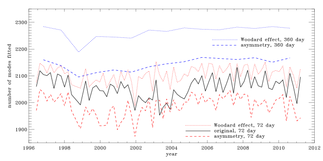
Figure 12.: Number of modes fitted as a function of time for the five different ways we analyzed the entire mission. Dotted lines show the set of all changes in the processing up to correcting for the Woodard effect; dashed lines show the result of also using asymmetric line profiles. In both cases the higher line is for the 360-day fits, the lower line is for the 72-day fits. The solid line shows the original analysis.

F-coverage

Figure 13.: Difference in frequency, amplitude, width, background parameter, $a_{1}$, and asymmetry parameter between 360-day fits and an average of 72-day fits as a function of frequency, in units of standard deviation from the 360-day fits. Dotted lines show the $\pm 1\sigma$ levels. The sense of subtraction is 360 day minus 72 day. At most 0.9 % of points have been excluded.

F-asym360d

Figure 14.: Ratio of the errors estimated from 360-day fits to the errors estimated from an average of 72-day fits as a function of frequency for the parameters shown in Figure F-asym360d. At most 1.9 % of points have been excluded.

F-asym360derr

Although the change in frequency seems to show a weak systematic dependence on frequency, the changes are mostly not significant. The change in frequency was slightly more significant using symmetric line profiles, especially at low frequencies. The changes in amplitude show ridge structure; although the majority of modes show reduced amplitude, the mean change is actually positive. The changes in width show ridges as well, but here the width is almost always less for the 360-day fits, and more so at lower frequencies. This is as one might expect, since the lorentzian is not well-resolved when the width is on the order of the width of a frequency bin. The increased frequency resolution of the 360-day fits better characterizes these low widths. The background parameter shows the most significant changes (an increase except for the $f$-mode), but centered on the $p$-mode band, where the noise is drowned by the signal. The changes in $a_{1}$ are the flattest, although a feature is discernible around 3.5 mHz. The asymmetry parameter was in general greater for the 360-day fits, with a peak around 1.8 mHz. For the frequency, width, and $a_{1}$, the estimated errors were much lower for the 360-day fits at low frequencies, again as one might expect. Harder to understand is why the error on the asymmetry parameter increased in the same frequency range. The background parameter also had lower errors, but again in the center of the frequency range.

4.2 Systematic Errors

S-syserrs

In this section we will refer to the changes in processing by the order in which they were applied. This is summarized in Table T-corrlist.

Table 2.: Sequence of changes made to the analysis; each analysis includes the changes made in all previous ones.

T-corrlist 0 original analysis 1 image scale 2 cubic distortion 3 CCD misalignment 4 inclination error 5 CCD tilt 6 window functions and detrending 7 gapfilling 8 horizontal displacement 9 distortion of eigenfunctions (“Woodard effect”) 10 asymmetric line profiles

To see the effect of the various changes on our systematic errors, we begin by performing simple one-dimensional regularized least-squares rotational inversions of the $a_{1}$-coefficient only. An RLS inversion seeks to minimize the sum of normalized residuals squared plus a penalty term that serves to constrain rapid variations in the solution. In particular, we have chosen to minimize

$$\ilabel{E-rls}\sum_{n\ell}\left[\frac{1}{\sigma_{1}(n,\ell)}\left(\int_{0}^{1}K_{n\ell}(r)\bar{\Omega}(r){\rm d}r-a_{1}(n,\ell)\right)\right]^{2}+\mu\int_{0}^{1}\left(\frac{{\mathrm{d}}^{2}\bar{\Omega}}{{\mathrm{d}}r^{2}}\right)^{2}{\rm d}r$$ (26)

where $\bar{\Omega}$ is the inferred rotation rate, the $K_{n\ell}$ are known kernels calculated from the mode eigenfunctions that relate the rotation rate to $a_{1}$, $\sigma_{1}$ is the standard error on $a_{1}$, $r$ is fractional radius, and $\mu$ is the tradeoff parameter that controls the relative importance of the two terms. A low value of $\mu$ will fit the data better, but the solution may oscillate wildly as a function of radius. A higher value of $\mu$ will attenuate this feature (the solution will be more regularized) at the cost of increased residuals (schou94inv). To choose a value of $\mu$, we have examined tradeoff curves, which are constructed by varying $\mu$ and plotting the rms of the residuals against the magnitude of the integral in the penalty term. The changes in $a_{1}$ that underlie the difference in the tradeoff curves for the different analyses were shown in Figure F-a1diff. The tradeoff curves themselves (shown in Figure F-tradeoff1) were computed using a modeset constructed by finding the modes common to all eleven analyses for each time interval and taking the average in time over whatever modes were present; in this case the errors used are the errors on the average.

Figure 15.: Tradeoff curves for several analyses. Dotted curve is for original analysis. Dash–dot curve shows first correction. Short-dashed curve shows first three corrections. Long-dashed curve shows first eight corrections (note this curve is above the one for only the first correction). Solid line is for all corrections. Symbols, from left to right, indicate tradeoff parameters of $\mu=10^{-4}$ and $\mu=10^{-9}$.

F-tradeoff1

As one can see, the image-scale correction made a substantial difference to the tradeoff curve. The curve for the cubic distortion correction is nearly indistinguishable. The correction for CCD misalignment made another significant reduction in the residuals, but the curves for the next four changes to the analysis all lie between the previous two. Accounting for the horizontal displacement caused a substantial increase in the residuals, but accounting for the Woodard effect resulted in the lowest curve shown. The use of asymmetric profiles made no change to the tradeoff curve. This is basically in line with what one might expect based on the differences in $a_{1}$ resulting from each change in the analysis shown in Figure F-a1diff.

To choose a value of $\mu$, one typically looks for the “elbow” in the tradeoff curve: the place where the residuals stop decreasing sharply, so that further decreases of $\mu$ will be of little benefit. Unfortunately, there seem to be two elbows in the curves shown in Figure F-tradeoff1. For the initial and final analyses, we have marked the point corresponding to the highest reasonable value of $\mu$ ($10^{-4}$) and the lowest value one might reasonably use ($10^{-9}$). Furthermore, if the model were a good fit to the data, for the lowest values of $\mu$ the tradeoff curve should approach a value of 1.0, which it does not.

In Figure F-bumps we show the normalized residuals of the inversions for the original and final analyses and for the smallest and largest values of $\mu$ given above. As one can see, the bump was mostly unaffected by all the changes in the analysis. A smaller value of $\mu$ decreases the size of the bump, but as Figure F-rotprof shows, the resulting rotation profile is unrealistic. The fact that the bump is only marginally present in the residuals for $\mu=10^{-9}$ suggests that this systematic error is responsible for the “knee” in the tradeoff curves. Notably, even this small value of $\mu$ was not able to fit the horns in the original analysis, which are greatly reduced in the final analysis. This is likely the cause of the overall reduction in $\chi^{2}$.

Figure 16.: Normalized residuals as a function of frequency. Top panels show original analysis, bottom panels show analysis with all changes applied. Left panels show $\mu=10^{-4}$, right panels show $\mu=10^{-9}$. The sense of subtraction is the opposite of Figure F-bumporig for ease of visual comparison.

F-bumps

Figure 17.: Internal rotation as a function of radius for the final analysis; curves for original analysis are similar. The solid line is the inversion result using $\mu=10^{-4}$; the dashed line uses $\mu=10^{-9}$.

F-rotprof

To investigate the annual periodicity in the $f$-mode frequency variations, we used the common modesets described above to fit a function of the form

$$f(t)=A\sin(\omega_{\rm yr}t)+B\cos(\omega_{\rm yr}t)+Ct+D$$ (27)

to the average fractional $f$-mode frequency shift relative to its average over time, where $\omega_{\rm yr}=2\pi/365.25$ and $t$ is measured in days. We did separate averaging and fits for four different ranges in degree [$\ell$]: 101 to 150, 151 to 200, 201 to 250, and 251 to 300. In each case, for each $\ell$ we took the average over whatever intervals it was fit in. Then, for each interval, we took the difference between each $\ell$ and the time average, divided by the time average, and then averaged over the range in $\ell$. We performed a weighted least-squares fit to this data, which yielded values for the parameters $A$, $B$, $C$, $D$, and their corresponding errors.

The images produced by MDI, however, are taken at equal intervals of time on the spacecraft, whereas it would be optimal if they were taken at equal intervals of time on the Sun. To correct for this effect, we applied the relativistic Doppler shift due to the motion of the spacecraft. That is, we multiplied each frequency and its error by $\sqrt{(c+v)/(c-v)}$ where $c$ is the speed of light and $v$ is the average velocity of the spacecraft away from the Sun, as derived from the OBS_VR keyword of the input dopplergrams for each 72-day interval. The resulting fits are shown in Figure F-phase, as well as the shift caused by the Doppler correction.

Figure 18.: Amplitude of cosine vs. sine component of annual periodicity for three analyses after Doppler correction: triangles show original analysis, diamonds show final analysis, and squares show the correction for cubic distortion, which yielded the largest amplitude of the annual component. Solid lines connect points for different ranges in $\ell$, beginning with the lowest range on the lower right. The arrow shows the size and direction of the shift resulting from the Doppler correction. The errors on $A$ and $B$ were similar for all analyses; the error bars show an average value. All values have been multiplied by $10^{6}$ to match the units in Figure F-radius.

F-phase

The amplitude of the annual component has a large variation between the different analyses, but in general it is always greater for the higher ranges in $\ell$. The point in the plot for $\ell$=251 – 300 of the original analysis contradicts that trend, but it must be noted that the fit represented by that point was an extremely poor one, which is likely related to the horns in the original analysis. For the lower two ranges in $\ell$, the amplitude was only marginally significant. Although not shown here, we note that the slope $C$ was zero for the lowest range in $\ell$, and becomes steadily more negative as $\ell$ increased, in agreement with previous findings [Antia et al. (2001)].

Finally, to explore the anomalous peak in the near-surface rotation rate near the poles (the high-latitude jet), we used the fits with 36 $a$-coefficients to perform two-dimensional RLS inversions for internal rotation. In this case we minimize

E-2drls$$\sum_{n\ell s}\left[\frac{1}{\sigma_{2s+1}(n,\ell)}\left(\int_{0}^{1}\int_{0}^{\pi}K_{n\ell s}(r,\theta)\bar{\Omega}(r,\theta){\rm d}r{\rm d}\theta-a_{2s+1}(n,\ell)\right)\right]^{2}+$$

$$\mu_{r}\int_{0}^{1}\left(\frac{{\mathrm{d}}^{2}\bar{\Omega}}{{\mathrm{d}}r^{2}}\right)^{2}{\rm d}r+\mu_{\theta}\int_{0}^{\pi}\left(\frac{{\mathrm{d}}^{2}\bar{\Omega}}{{\mathrm{d}}\theta^{2}}\right)^{2}{\rm d}\theta$$ (28)

in perfect analogy with Equation (E-rls) [Schou, Christensen-Dalsgaard, and Thompson (1994)]. We formed common modesets and averaged them using the same method described above for one-dimensional inversions, and used tradeoff parameters of $\mu_{r}=10^{-6}$ and $\mu_{\theta}=10^{-2}$ for the radial and latitudinal regularization terms respectively. Using this relatively high value for $\mu_{\theta}$ should dampen variations in latitude [Howe et al. (2000)]. The results are shown in Figure F-jet; the jet is more pronounced in this plot than in Figure F-rot2d, which can be attributed both to the different modeset and to the smaller errors resulting from averaging. Although in every updated analysis the polar jet actually had a greater magnitude than in the original analysis, the gapfilling resulted in a reduced rotation rate in the lower convection zone, which brings our result closer to agreement with inferences drawn by the GONG analysis [Schou et al. (2002)].

Figure 19.: Internal rotation as a function of radius at $75^{\circ}$ latitude for three analyses. Solid lines show the original analysis and its error bars; errors on the other analyses are similar. The dotted curve is the analysis that includes the improved gapfilling, and the dashed curve is the final analysis.

F-jet

5 Discussion and Future Prospects

S-discussion

We have found that the various changes that we made to the processing of medium-$\ell$ data from MDI resulted in significant changes in mode parameters. In summary, changes in width were overall the least significant, followed by the changes in $a_{1}$, which mostly resulted from correcting for the distortion of eigenfunctions by the differential rotation (the Woodard effect). The background was largely unaffected by most changes except the improved detrending and gapfilling. The image-scale correction made the dominant changes to the amplitudes and frequencies. For the latter, large changes also resulted from accounting for asymmetry, horizontal displacement, the Woodard effect, and cubic distortion, in decreasing order of significance.

Not only is one led to believe these changes represent an improvement as a matter of principle, but some of the systematic errors in the analysis have been reduced as well. In particular, the horns have been greatly reduced, resulting in overall lower residuals from rotational inversions. A more stubborn systematic error is the bump in the odd $a$-coefficients, which seems to be reflected in the anomalous shape of the tradeoff curve. This remained almost completely unchanged in all analyses. Nor did any change to the analysis make a reduction in the high-latitude jet just below the solar surface, although there is an improved agreement with GONG in the lower convection zone.

Regarding the annual periodicity in the $f$-mode frequencies, we found that the first change that we applied, the image-scale correction, resulted in a drastically increased magnitude of the annual component for the higher two ranges in $\ell$. The correction for cubic distortion resulted in an even higher amplitude. After correcting for the misalignment of the CCD, however, the amplitude was reduced and did not vary much for later changes. We conjecture that the original fits were so poor at high $\ell$ (thus the horns) that the one-year period was swamped by noise there. The image-scale correction, which was the most significant one for the frequencies, itself has a one-year period due to its dependence on observer distance. Hence this correction revealed the remaining annual periodicity in the $f$-mode frequencies, which appears to result mostly from errors in $P_{\rm eff}$. Due to symmetry, one would expect the frequency error to depend on the absolute value of the error in $P_{\rm eff}$. The inclination error by itself would therefore be expected to result in a six-month period, but the combination with the misalignment of the CCD causes a one-year period. Hence, although the correction for CCD misalignment is constant in time, it still greatly reduces the annual component.

Of concern to us is the discrepancy between the 360-day analysis, which in principle should be more accurate, and the 72-day analysis. Most notably, it indicates a problem with our model of the background. Interestingly, the asymmetry was the only parameter for which the error was greater for the 360-day fits (at low frequency), and adding the asymmetry also made significant changes to the background and its error.

In spite of these shortcomings, the analysis of the MDI data in its entirety allows us to determine mode parameters with extraordinary precision. This is illustrated in Figure F-lnu, where we show mode coverage in the $\ell$–$\nu$ plane along with the estimated uncertainty on the frequencies.

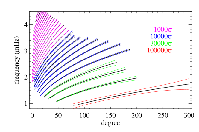
Figure 20.: An $\ell$-$\nu$ diagram with magnified errors. Dots represent a mode that was fitted in at least 12 of the 15 years we analyzed using symmetric profiles. Solid lines show the errors: for the $f$-mode, these have been multiplied by 100 000. For $n=1,2,3$ the errors have been multiplied by 30 000. The next eight ridges ($n=4\,-\,11$) have errors multiplied by 10 000. The remaining ridges have errors multiplied by 1000.

F-lnu

Although our analysis has in general been very successful, the core peakbagging routines were written at a time when computational capabilities were far less than now. A number of approximations which were necessary 20 years ago could now be lifted. The current work is an attempt to remove some of these limitations. Over the years, other workers in the field have also made contributions to the problem of inferring physical properties of the Sun from medium-$\ell$ MDI data. vorontsov13 have proposed fitting power spectra for rotation directly, circumventing the need to measure frequencies. As an intermediate step they have still done so, using more physically motivated spectral models and an analytically calculated leakage matrix. korzennik05 has used sine multi-tapers as power-spectrum estimators and fit widths and asymmetries as functions of $m$. johan have fit $m$-averaged spectra using a methodology that extends to high $\ell$.

A potential difficulty facing these efforts is the computation of the leakage matrix. In general, the use of a leakage matrix should increase the stability of fits, but the results will then depend upon the assumptions that went into its calculation. In particular, one might consider using leakage matrices calculated for different observer distances and values of $B_{0}$. This has been done explicitly by korzennik13 and analytically by vorontsov13. Others have attempted to fit the coupling of modes by subsurface flows, among them schad13 and woodard13.

Although a comparison between the results of these other investigators and our improved analysis is still pending, all agree that some systematic errors remain in every analysis. These have been variously attributed to anisotropy in the point-spread function of MDI, failure to account for the height of formation in the solar atmosphere of the observed spectral line or the difference in light travel time between disk center and limb, and the effect of convective flows on the phase of the oscillations.

For us, there are a number of ways to move forward. The most obvious is the extension of this work to other datasets. First and foremost of these must be the MDI full-disk data, which will allow us to determine how systematic errors and mode parameters might depend on the smoothing of the medium-$\ell$ data and its apodization. Because of its duty cycle the full-disk data cannot be used to study the annual periodicity in our results, but now the Helioseismic and Magnetic Imager (HMI: hmi) onboard the Solar Dynamics Observatory (SDO) has taken a long enough span of data for it to be suitable for this purpose. Phil Scherrer (private communication, 2014) has suggested that the one year period may be related to the variable (in solar coordinates) width of the gaussian used for smoothing the medium-$\ell$ data; an analysis of the MDI medium-$\ell$ proxy from HMI should elucidate the issue. Finally, a repetition of the comparison with GONG results is long overdue. The original comparisons all used GONG classic data; now that GONG+ (gongplus) has been in place for over 13 years and software pipelines in both projects have been updated, the time has come to renew an investigation of the systematic differences between the two.

There still remain possibilities for progress with the MDI medium-$\ell$ dataset itself. One that is suggested by the results of this article is to correct the timeseries for the relative motions of SOHO and the Sun. Although we can correct the frequencies after the fitting by Doppler shifting them, there is no obvious way to correct the other mode parameters. Another change in the analysis that suggests itself is to the width of the fitting window, since this is one of the things most notably different in the GONG analysis and is also known to affect the shape of the bump in the $a$-coefficients. During the remapping performed prior to spherical harmonic decomposition, we could implement an interpolation algorithm that takes into account the correlation between points introduced by the gaussian smoothing. We have also considered the common practice of zero-padding our timeseries before performing Fourier transforms. Lastly, the parameter space of the detrending and gapfilling remains almost entirely unexplored.

Acknowledgements

This work was supported by NASA Contract NAS5-02139. SOHO is a mission of international cooperation between NASA and ESA. The authors thank the Solar Oscillations Investigation team at Stanford University and its successor, the Joint Science Operations Center. We thank Rasmus Larsen in particular for providing the gapfilling code. Much of the work presented here was done while J. Schou was at Stanford University. T.P. Larson thanks the Max-Planck-Institut für Sonnensystemforschung for generously hosting him during the composition of this article.

Disclosure of Potential Conflicts of Interest The authors declare that they have no conflicts of interest.

Detailed information on how to access MDI data from the global helioseismology pipeline can be found on the website of the Joint Science Operations Center (JSOC) at http://jsoc.stanford.edu/MDI/MDI˙Global.html. This page contains documentation describing how the datasets used in this article were made and how they can be remade. In this appendix we describe how to access the relevant archived data. In what follows we assume some familiarity with the Data Record Management System (DRMS), detailed documentation for which is linked from the above website.

Mode parameter files (as ASCII tables) for every analysis discussed in this paper are available in the electronic supplementary material. For the original analysis, they (and a helpful Readme file) can also be found at http://sun.stanford.edu/~schou/anavw72z/. For all other analyses, they can also be retrieved from JSOC. The fields of a mode-parameter file are the following: $\ell$, $n$, $\nu_{0}$, $A$, $w$, $b$, $x$, $\{\tan(\gamma)\}$, $\sigma_{\nu_{0}}$, $\sigma_{A}$, $\sigma_{w}$, $\sigma_{b}$, $\sigma_{x}$, $\{\sigma_{\tan(\gamma)}\}$, $a_{1}$, $a_{2}$, … $a_{N}$, $\sigma_{1}$, $\sigma_{2}$, … $\sigma_{N}$. The parameter $\tan(\gamma)$ and its error will not be present for fits done with symmetric profiles. The value of $N$ is either 6, 18, or 36. Any parameter with zero error has not been fit for. The parameter $x$ is not fit for in these analyses and is retained for historical reasons.

The data for the different “corrections” are labelled by the strings corr1 to corr9 corresponding to the numbering scheme in Table T-corrlist. The final correction in this set refers to the first way of applying the Woodard effect (holding $B_{1}$ and $B_{2}$ constant). These data have all been generated in the first author’s name space, with mode parameters found in su_tplarson.corr_vw_V_sht_modes. The primekeys are T_START, LMIN, LMAX, NDT, and TAG, where T_START is the beginning of the corresponding timeseries, most easily specified by the MDI day number suffixed by “d” (see Table T-data). For all records in this series, LMIN=0, LMAX=300, and NDT=103680, so these primekeys need never be specified. The TAG keyword is the label string, so TAG and T_START uniquely specify every record.

The second way of applying the Woodard effect, as well as the asymmetric fits, are both represented in the official MDI name space (mdi). For the former, mode parameters can be found in mdi.vw_V_sht_modes and for the latter in mdi.vw_V_sht_modes_asym. The primekeys are the same as given above, with the exception that these series do not have the TAG keyword and that NDT=518400 for the 360-day fits. In addition, the results used in this article have the VERSION keyword (not a primekey) in these series set to version2. If these data are reprocessed in the future, VERSION will get a new value, but old versions can easily be retrieved.

The dataseries containing timeseries and window functions in the mdi name space have also been archived and can be retrieved; details on these data products are given on the above website. The corresponding data in the su_tplarson name space have not been archived, but can be recreated if needed. The procedure for doing so can be found on the website. The original timeseries and window functions have been archived in the dsds namespace, but have not yet been ported to the standard DRMS format for global helioseismology data products. They can, however, still be retrieved by request.

References

- Anderson, Duvall, and Jefferies (1990) Anderson, E.R., Duvall, T.L. Jr., Jefferies, S.M.: 1990, Modeling of solar oscillation power spectra. ApJ 364, 699. DOI. ADS.
- Antia et al. (2001) Antia, H.M., Basu, S., Pintar, J., Schou, J.: 2001, How correlated are f-mode frequencies with solar activity? In: Wilson, A., Pallé, P.L. (eds.) SOHO 10/GONG 2000 Workshop: Helio- and Asteroseismology at the Dawn of the Millennium, SP-464, ESA, Noordwijk, 27. ADS.
- Beck and Giles (2005) Beck, J.G., Giles, P.: 2005, Helioseismic Determination of the Solar Rotation Axis. ApJ 621, L153. DOI. ADS.
- Christensen-Dalsgaard (2004) Christensen-Dalsgaard, J.: 2004, An Overview of Helio- and Asteroseismology. In: Danesy, D. (ed.) SOHO 14 Helio- and Asteroseismology: Towards a Golden Future, SP-559, ESA, Noordwijk, 1. ADS.
- Duvall (1982) Duvall, T.L. Jr.: 1982, A dispersion law for solar oscillations. Nature 300, 242. DOI. ADS.
- Duvall et al. (1993) Duvall, T.L. Jr., Jefferies, S.M., Harvey, J.W., Osaki, Y., Pomerantz, M.A.: 1993, Asymmetries of solar oscillation line profiles. ApJ 410, 829. DOI. ADS.
- Fahlman and Ulrych (1982) Fahlman, G.G., Ulrych, T.J.: 1982, A New Method for Estimating the Power Spectrum of Gapped Data. MNRAS 199, 53. ADS.
- Gough (2013) Gough, D.: 2013, What Have We Learned from Helioseismology, What Have We Really Learned, and What Do We Aspire to Learn? Sol. Phys. 287, 9. DOI. ADS.
- Harvey et al. (1996) Harvey, J.W., Hill, F., Hubbard, R.P., Kennedy, J.R., Leibacher, J.W., Pintar, J.A., Gilman, P.A., Noyes, R.W., Title, A.M., Toomre, J., Ulrich, R.K., Bhatnagar, A., Kennewell, J.A., Marquette, W., Patron, J., Saa, O., Yasukawa, E.: 1996, The Global Oscillation Network Group (GONG) Project. Science 272, 1284. DOI. ADS.
- Hill et al. (2003) Hill, F., Bolding, J., Toner, C., Corbard, T., Wampler, S., Goodrich, B., Goodrich, J., Eliason, P., Hanna, K.D.: 2003, The GONG++ data processing pipeline. In: Sawaya-Lacoste, H. (ed.) GONG+ 2002. Local and Global Helioseismology: the Present and Future, SP-517, ESA, Noordwijk, 295. ADS.
- Howe et al. (2000) Howe, R., Christensen-Dalsgaard, J., Hill, F., Komm, R.W., Larsen, R.M., Schou, J., Thompson, M.J., Toomre, J.: 2000, Deeply Penetrating Banded Zonal Flows in the Solar Convection Zone. ApJ 533, L163. DOI. ADS.
- Korzennik (2005) Korzennik, S.G.: 2005, A Mode-Fitting Methodology Optimized for Very Long Helioseismic Time Series. ApJ 626, 585. DOI. ADS.
- Korzennik and Eff-Darwich (2013) Korzennik, S.G., Eff-Darwich, A.: 2013, Mode Frequencies from 17, 15 and 2 Years of GONG, MDI, and HMI Data. J. Phys. CS-440(1), 012015. DOI. ADS.
- Korzennik, Rabello-Soares, and Schou (2004) Korzennik, S.G., Rabello-Soares, M.C., Schou, J.: 2004, On the Determination of Michelson Doppler Imager High-Degree Mode Frequencies. ApJ 602, 481. DOI. ADS.
- Larson and Schou (2009) Larson, T., Schou, J.: 2009, Variations in Global Mode Analysis. In: Dikpati, M., Arentoft, T., González Hernández, I., Lindsey, C., Hill, F. (eds.) Solar-Stellar Dynamos as Revealed by Helio- and Asteroseismology: GONG 2008/SOHO 21, CS-416, Astron. Soc. Pac., San Franscisco, 311. ADS.
- Larson and Schou (2008) Larson, T.P., Schou, J.: 2008, Improvements in global mode analysis. J. Phys. CS-118(1), 012083. DOI. ADS.
- Libbrecht (1992) Libbrecht, K.G.: 1992, On the ultimate accuracy of solar oscillation frequency measurements. ApJ 387, 712. DOI. ADS.
- Nigam and Kosovichev (1998) Nigam, R., Kosovichev, A.G.: 1998, Measuring the Sun’s Eigenfrequencies from Velocity and Intensity Helioseismic Spectra: Asymmetrical Line Profile-fitting Formula. ApJ 505, L51. DOI. ADS.
- Reiter et al. (2015) Reiter, J., Rhodes, E.J. Jr., Kosovichev, A.G., Schou, J., Scherrer, P.H., Larson, T.P.: 2015, A Method for the Estimation of p-Mode Parameters from Averaged Solar Oscillation Power Spectra. ApJ 803, 92. DOI. ADS.
- Rhodes et al. (2001) Rhodes, E.J. Jr., Reiter, J., Schou, J., Kosovichev, A.G., Scherrer, P.H.: 2001, Observed and Predicted Ratios of the Horizontal and Vertical Components of the Solar p-Mode Velocity Eigenfunctions. ApJ 561, 1127. DOI. ADS.
- Schad, Timmer, and Roth (2013) Schad, A., Timmer, J., Roth, M.: 2013, Global Helioseismic Evidence for a Deeply Penetrating Solar Meridional Flow Consisting of Multiple Flow Cells. ApJ 778, L38. DOI. ADS.
- Scherrer et al. (1995) Scherrer, P.H., Bogart, R.S., Bush, R.I., Hoeksema, J.T., Kosovichev, A.G., Schou, J., Rosenberg, W., Springer, L., Tarbell, T.D., Title, A., Wolfson, C.J., Zayer, I., MDI Engineering Team: 1995, The Solar Oscillations Investigation - Michelson Doppler Imager. Sol. Phys. 162, 129. DOI. ADS.
- Schou (1992) Schou, J.: 1992, On the Analysis of Helioseismic Data. PhD thesis, Aarhus University, Aarhus, Denmark. ADS.
- Schou (1999) Schou, J.: 1999, Migration of Zonal Flows Detected Using Michelson Doppler Imager F-Mode Frequency Splittings. ApJ 523, L181. DOI. ADS.
- Schou and Bogart (2002) Schou, J., Bogart, R.S.: 2002, Reduction of Systematic Errors in MDI Measurements. In: American Astronomical Society Meeting Abstracts #200, Bull. Amer. Astron. Soc. 34, 645. ADS.
- Schou and Brown (1994) Schou, J., Brown, T.M.: 1994, Generation of artificial helioseismic time-series. A&AS 107, 541. ADS.
- Schou, Christensen-Dalsgaard, and Thompson (1994) Schou, J., Christensen-Dalsgaard, J., Thompson, M.J.: 1994, On comparing helioseismic two-dimensional inversion methods. ApJ 433, 389. DOI. ADS.
- Schou et al. (2002) Schou, J., Howe, R., Basu, S., Christensen-Dalsgaard, J., Corbard, T., Hill, F., Komm, R., Larsen, R.M., Rabello-Soares, M.C., Thompson, M.J.: 2002, A Comparison of Solar p-Mode Parameters from the Michelson Doppler Imager and the Global Oscillation Network Group: Splitting Coefficients and Rotation Inversions. ApJ 567, 1234. DOI. ADS.
- Schou et al. (2012) Schou, J., Scherrer, P.H., Bush, R.I., Wachter, R., Couvidat, S., Rabello-Soares, M.C., Bogart, R.S., Hoeksema, J.T., Liu, Y., Duvall, T.L., Akin, D.J., Allard, B.A., Miles, J.W., Rairden, R., Shine, R.A., Tarbell, T.D., Title, A.M., Wolfson, C.J., Elmore, D.F., Norton, A.A., Tomczyk, S.: 2012, Design and Ground Calibration of the Helioseismic and Magnetic Imager (HMI) Instrument on the Solar Dynamics Observatory (SDO). Sol. Phys. 275, 229. DOI. ADS.
- Vorontsov (2007) Vorontsov, S.V.: 2007, Solar p modes of high degree l: coupling by differential rotation. MNRAS 378, 1499. DOI. ADS.
- Vorontsov and Jefferies (2013) Vorontsov, S.V., Jefferies, S.M.: 2013, Modeling Solar Oscillation Power Spectra. II. Parametric Model of Spectral Lines Observed in Doppler-velocity Measurements. ApJ 778, 75. DOI. ADS.
- Woodard (1989) Woodard, M.F.: 1989, Distortion of high-degree solar p-mode eigenfunctions by latitudinal differential rotation. ApJ 347, 1176. DOI. ADS.
- Woodard et al. (2013) Woodard, M., Schou, J., Birch, A.C., Larson, T.P.: 2013, Global-Oscillation Eigenfunction Measurements of Solar Meridional Flow. Sol. Phys. 287, 129. DOI. ADS.