Doppler shift of the quiet region measured by meridional scans with the EUV Imaging Spectrometer onboard Hinode

Abstract

Spatially averaged ($>50^{\prime\prime}$) EUV spectral lines in the transition region of solar quiet regions are known to be redshifted. Because the mechanism underlying this phenomenon is unclear, we require additional physical information on the lower corona for limiting the theoretical models. To acquire this information, we measured the Doppler shifts over a wide coronal temperature range ($\log T\,[\mathrm{K}]=5.7$–$6.3$) using the spectroscopic data taken by the Hinode EUV Imaging Spectrometer. By analyzing the data over the center-to-limb variations covering the meridian from the south to the north pole, we successfully measured the velocity to an accuracy of $3\,\mathrm{km}\,\mathrm{s}^{-1}$. Below $\log T\,[\mathrm{K}]=6.0$, the Doppler shifts of the emission lines were almost zero with an error of $1$–$3\,\mathrm{km}\,\mathrm{s}^{-1}$; above this temperature, they were blueshifted with a gradually increasing magnitude, reaching $-6.3\pm 2.1\,\mathrm{km}\,\mathrm{s}^{-1}$ at $\log T\,[\mathrm{K}]=6.25$.

1 Introduction

The emission lines formed in the transition region of the solar quiet regions show redshifted features (e.g., Doschek et al., 1976; Brekke et al., 1997; Chae et al., 1998; Peter & Judge, 1999; Teriaca et al., 1999). The magnitude of the redshift increases with increasing temperature, with a peak of approximately $10\,\mathrm{km}\,\mathrm{s}^{-1}$ at $10^{5}\ \mathrm{K}$ and then decreases at higher temperatures. Using the Solar Ultraviolet Measurement of Emitted Radiation (SUMER) instruments of the Solar Heliospheric Observatory (SoHO) spacecraft, Peter & Judge (1999) found blueshifts for three coronal lines ($-(2.4$–$3)\pm 1\,\mathrm{km}\,\mathrm{s}^{-1}$ for Ne viii and $-4.5\pm 3\,\mathrm{km}\,\mathrm{s}^{-1}$ for Mg x); while Chae et al. (1998) showed that the same lines are redshifted ($+5.3\pm 1\,\mathrm{km}\,\mathrm{s}^{-1}$ for Ne viii and $+3.8\,\mathrm{km}\,\mathrm{s}^{-1}$ for Mg x). These observations suggest prevalent mass motion in the heights of the observed Doppler-shifted emission lines. To understand this motion, precise measurements within an accuracy of a few $\mathrm{km}\,\mathrm{s}^{-1}$ are required.

The EUV Imaging Spectrometer (EIS; Culhane et al. 2007) onboard Hinode (Kosugi et al., 2007) measures Doppler shifts in the solar corona and the transition region with an unprecedentedly high accuracy. The CCD pixel size of the EIS detector corresponds to $22\,\mathrm{m\AA}$ ($33\,\mathrm{km}\,\mathrm{s}^{-1}$ for 200 Å line) . By fitting a model function to an observed profile in a band window with more than ten pixels, the precision can be improved to within a few $\mathrm{km}\,\mathrm{s}^{-1}$ in a statistical sense. Since EIS has no onboard system for absolute wavelength calibration, the line centroid wavelength in a quiet region of the field of view (FOV) is frequently designated the zero-velocity point.

Measurements of Doppler shifts contain several uncertainties. First, uncertainty exists in the rest wavelengths of some emission lines, whether theoretically or experimentally derived. The NIST database shows that the rest wavelengths are precise to the order of $10^{-2}$Å ($15\,\mathrm{km}\,\mathrm{s}^{-1}$ for 200 Å line) in most cases, slightly larger than our current requirement. Second is the uncertainty in the instrument’s observing conditions: The grating component displaces with the thermal environmental change of the Hinode spacecraft, thus causing drift of the spectral signals on the CCDs (Brown et al., 2007). The SolarSoftware package developed by Kamio et al. (2010) is widely used to correct the wavelength scale in EIS analysis, but residuals of $4$–$5\,\mathrm{km}\,\mathrm{s}^{-1}$ remain in the standard deviation. Third is the choice of the zero-velocity reference. Many analyses assume zero Doppler shift for the averaged profile in a quiet region of the emission line Fe xii $195.12$Å. However, this choice is simply an assumption without any concrete physical reasoning.

To avoid the above mentioned difficulties, we measured the center-to-limb behavior of the Doppler shift. This calibration is especially useful for determining the zero-velocity wavelength of each spectral line (e.g., Roussel-Dupré & Shine, 1982). Applying this approach, Peter (1999) and Peter & Judge (1999) obtained the redshift features in the transition region lines and the blueshift tendency of the coronal lines from SUMER data. Combining the observations of different instruments (such as SUMER and EIS) is also useful when one of the instruments (in this case, SUMER) has a substantially small uncertainty with a reliable calibration method, e.g., in case of SUMER, that is by using chromospheric lines and its counterpart well-determined telluric lines (Samain, 1991). Dadashi et al. (2011) conducted this analysis and obtained the Doppler shift of spectral lines formed between 1 and 2 MK in the quiet corona for the first time.

In this paper, we analyze the EIS data covering the meridian from the south to the north pole, and measure the Doppler shifts from the center-to-limb behavior of each emission line. Our measurements are precise to within $3\,\mathrm{km}\,\mathrm{s}^{-1}$. By using this technique, not only relative but also absolute calibration becomes possible irrespective of the uncertainties in the line database and in the instrumental thermal drift. Besides improving the precision, the EIS observations can provide new information of the Doppler shift over higher temperature ranges. These independent measurements with independent assumptions can be compared with those of Dadashi et al. (2011) for better diagnostics of the Doppler signals.

The rest of this paper is organized as follows. Section 2 describes the data and observational setup. Section 3 is devoted to our data reduction procedures. Results and discussion are given in Section 4 and 5, respectively. The Appendix details the selection process of the emission lines and presents examples of their profiles.

2 Observations

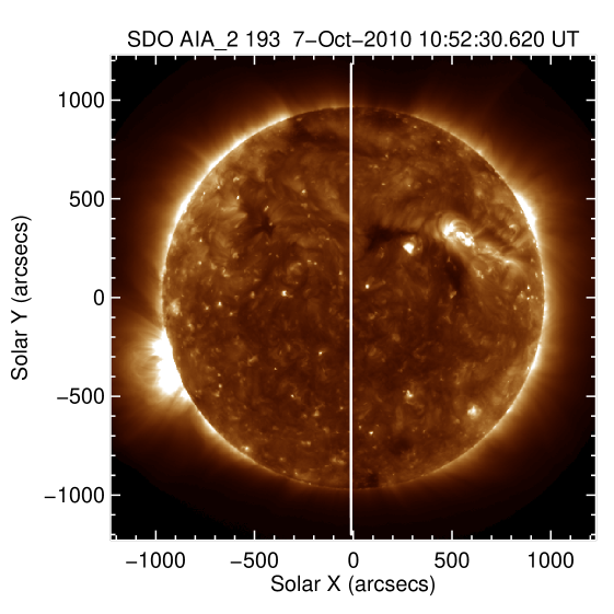
Figure 1: SDO/AIA $193$Å passband image at the start of the October sequence of HOP79. The white vertical line indicates the location of spectral data measurements by EIS.

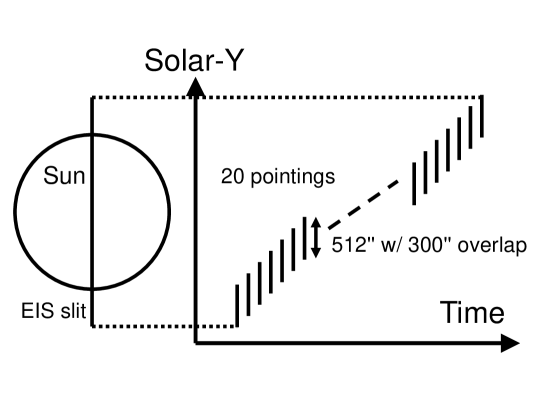
Figure 2: Schematic of north–south scanning in HOP79.

We used the EIS spectral data of the north–south scans along the solar meridian acquired by the Hinode Observing Plan 79 (HOP79). Figure 1 shows the context image with a white line indicating the location of EIS spectral data. The pointing procedure in this observation is schematized in Figure 2. Using the $1^{\prime\prime}\times 512^{\prime\prime}$ slit, five exposures with $1^{\prime\prime}$ offset were conducted at each pointing. The slit is oriented in the north-south direction, i.e., the solar-$y$ direction of the heliocentric coordinate. The pointing was shifted in the north-south direction with an overlap of $300^{\prime\prime}$. In this way, we could investigate the center-to-limb variation of the Doppler shifts of the emission lines by mutual calibration among the overlapping scans. The exposure time ($120\,\mathrm{s}$) was sufficient for an appropriate signal-to-noise (S/N) ratio for many coronal emission lines even in the quiet region. The EIS study consisted of 16 spectral windows with widths of $24$–$48$ pixels ($\simeq 0.5$–$1.0$Å).

We analysed the spectral data in October 7–8 and December 2–3 of 2010. During this period, the solar activity was relatively low and the observed area contained no large coronal hole, thus enabling us to avoid the influence of these regions and to focus only on the quiet regions. Note that, although the data was carefully chosen to avoid brighter loops, the analysed quiet region still has structures and complex magnetic connectivity as seen in Fig. 1.

3 Data reduction and analysis

Eleven of the observed emission lines were selected for a detailed analysis of their Doppler shifts (Table 1). The selection was made by comparing the line profiles at two locations; beyond the solar limb and on the disk. When the emission-line intensity signal was significantly larger in the disk observation than in the area beyond the limb, the emission line was selected for further analysis. Emission lines with known blending effects from neighboring lines were also removed from the candidates. The details of the selection process are presented in the Appendix.

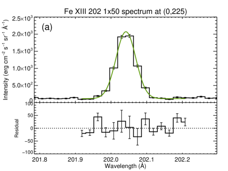
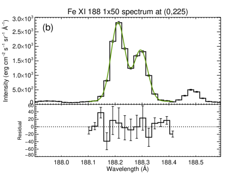
Figure 3: Examples of the observed emission lines and their fitting results. (a) Fe xiii $202.04$Å and (b) Fe xi $188.21$Å/$188.30$Å in the October observation sequence. The observational data is in the histograms, and the fitted functions are in solid green lines in the upper subpanels. Lower subpanels show the fitting residuals with error bars over the fitting range. The error bars include photon noise and uncertainty in the CCD pedestal and dark current.

Each emission line was fitted to a Gaussian function. Prior to the fitting, the spectra were spatially integrated over $50^{\prime\prime}$ in the solar-$y$ direction to reduce the fluctuations introduced by coronal structures (e.g., bright points) and non-radial motions. An example is shown in Figure 3(a). The residuals are within $\sim 2$% of the peak in the spectrum and are comparable to the photon noise. Most of the eleven selected lines were fitted by a single-component Gaussian function. The fitting range of the wavelength was $8$–$14$ pixels including the line centroid. The Fe xi $188.21$Å and $188.30$Å lines, which overlap, were combined and simultaneously fitted by a double-component Gaussian function (Fig. 3b).

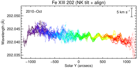
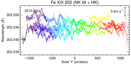
Figure 4: Line centroid wavelength as functions of solar-$y$. Different colors indicate data collected at different north-south pointings ($20$ locations). Note that each data segment for each pointing is represented by a unique color (i.e., each of the 20 colors represents one of the 20 segments) . The apparent gradation behavior is attributed to overlapping segments. Top: Data calibrated by our alignment procedure described in the text. Bottom: Data calibrated by the standard procedure provided by the SolarSoftware package.

The wavelengths of each exposure and pointing are relatively offset from each other. We removed these offsets by the following procedures: (1) Five profiles in the exposures in each north-south pointing were aligned by changing their wavelength scales to remove their (albeit tiny) relative offsets, and (2) the aligned profiles for each pointing were further aligned with their neighboring ones using the profiles in the spatially overlapping observing regions. An example of an alignment is shown in the top panel of Figure 4. For comparison, the results of the standard SolarSoftware package are presented in the bottom panel. After our alignment procedures, the line centroid wavelengths were consistent within $0.002$Å ($\simeq 3\,\mathrm{km}\,\mathrm{s}^{-1}$), thus demonstrating clear improvement over the standard procedure.

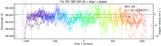
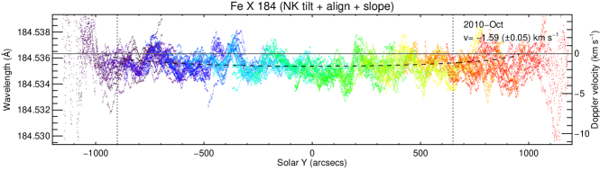
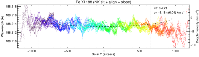
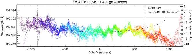
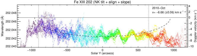
Figure 5: Centroid wavelengths of the emission lines as functions of solar-$y$, i.e., the center-to-limb variation of the Doppler shift. Each panel represents a different emission line: (a) Fe viii $186.60$Å, (b) Fe x $184.54$Å, (c) Fe xi $188.21$Å, (d) Fe xii $192.39$Å, and (e) Fe xiii $202.04$Å. In each panel, the dashed line is the fitting curve based on the radial flow model, and the vertical dotted lines indicate the fitting range.

Figure 5 plots the Doppler shifts as functions of solar-$y$. The final procedure calibrates the absolute velocity; in other words, the zero-velocity wavelength determination. Here, the spatial distribution of the Doppler shift was fitted by a radial flow model of the form $v(\theta)=v_{0}\cos\theta$ where $v_{0}$ is the radial velocity and $\theta$ is the angle between the line of sight and the normal to the solar surface. The solar-$y$ is represented as $y=R_{\odot}\sin\theta$. To fit the data, we converted the abscissa into $\cos\theta$ and applied a linear function. One of the fitting parameters was the interception (i.e., wavelength shift) of the fitting line at the limb ($\cos\theta=0$). The obtained finite interception was used to correct the entire distribution assuming zero Doppler shift at the limb. After this correction, the Doppler shift at the disk center corresponded to the outflow velocity $v_{0}$. The fitting was done within the range indicated by the region between the two vertical dotted lines in Fig.  5. The fitting error in $v_{0}$ was $\sigma_{\mathrm{fit}}<0.1\,\mathrm{km}\,\mathrm{s}^{-1}$. Note that there is a small coronal hole at the north pole and the emission lines are clearly blueshifted at $y\geq 700^{\prime\prime}$, indicating possible outflow. The radial velocity at the disk center (stated in the upper-right corner of each panel in Fig. 5) reveals an increasing magnitude of the shift (i.e., stronger upflows) as the line-formation temperature increases.

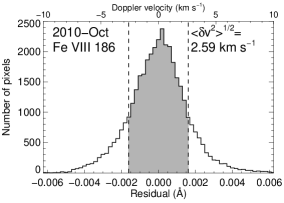
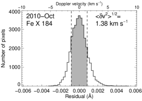
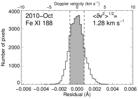
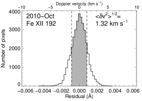
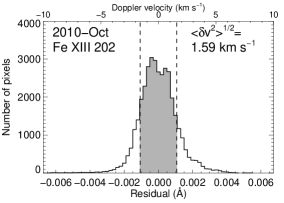
Figure 6: Histograms of deviation in the actual Doppler shifts from the fittings based on the radial flow model (Fig. 5). Results are plotted for the Fe viii, and x–xiii lines. Numbers in the upper-right corners are the standard deviations $\langle\delta v^{2}\rangle^{1/2}$, also shown by the vertical dashed lines.

Figure 6 shows histograms of the deviation in the Doppler shift from the fitted radial flow model (Fig. 5). The standard deviation was $\langle\delta v^{2}\rangle^{1/2}=1\text{--}3\,\mathrm{km}\,\mathrm{s}^{-1}$. This finite deviation $\langle\delta v^{2}\rangle^{1/2}$, which should include the real flow fluctuations in the solar quiet regions, affects our fitting results of the radial flow speed $v_{0}$. Because we computed the averaged flow speed beyond such spatial or temporal fluctuations, we took $\sigma_{\mathrm{tot}}=\left(\sigma_{\mathrm{fit}}^{2}+\langle\delta v^{2}\rangle\right)^{1/2}$ as the error in our estimated radial velocity $v_{0}$.

4 Results

Table 1: Radial velocity $v_{0}$ ($\mathrm{km}\,\mathrm{s}^{-1}$) in our fitting model (interpretable as the Doppler velocity at the disk center). $\sigma_{\mathrm{fit}}$ is the error in the fitted velocity and $\langle\delta v^{2}\rangle^{1/2}$ is the standard deviation relative to the fitted curve. The symbol ^b appended to the wavelength (denoted by Wvl. in the second column) means that the emission line is potentially blended with another emission line.

			Radial velocities and their errors ($\mathrm{km}\,\mathrm{s}^{-1}$)
			October			December
Ion	Wvl. (Å)	$\log T\,[\mathrm{K}]$	$v_{0}$	$\sigma_{\mathrm{fit}}$	$\langle\delta v^{2}\rangle^{1/2}$	$v_{0}$	$\sigma_{\mathrm{fit}}$	$\langle\delta v^{2}\rangle^{1/2}$
Fe viii	$186.60$	$5.69$	$-1.57$	$0.09$	$2.59$	$-0.35$	$0.13$	$2.85$
Si vii	$275.35$	$5.80$	$-2.45$	$0.10$	$2.86$	$4.56$	$0.16$	$3.41$
Fe ix	$188.49$	$5.92$	$1.00$	$0.06$	$1.73$	$1.55$	$0.09$	$1.92$
Fe x	$184.54$	$6.04$	$-1.59$	$0.05$	$1.38$	$-1.84$	$0.06$	$1.37$
	$257.26$		$-3.63$	$0.08$	$2.05$	$-2.09$	$0.09$	$1.91$
Fe xi	$180.40^{\mathrm{b}}$	$6.12$	$-2.24$	$0.07$	$2.07$	$0.48$	$0.09$	$2.00$
	$188.21$		$-3.18$	$0.04$	$1.28$	$-1.12$	$0.06$	$1.27$
	$188.30$		$-3.26$	$0.06$	$1.34$	$-0.44$	$0.06$	$1.31$
Fe xii	$192.39$	$6.19$	$-5.49$	$0.05$	$1.32$	$-3.18$	$0.06$	$1.28$
	$195.12^{\mathrm{b}}$		$-2.38$	$0.05$	$1.29$	$-0.05$	$0.07$	$1.44$
Fe xiii	$202.04$	$6.25$	$-6.66$	$0.06$	$1.59$	$-6.57$	$0.09$	$1.91$

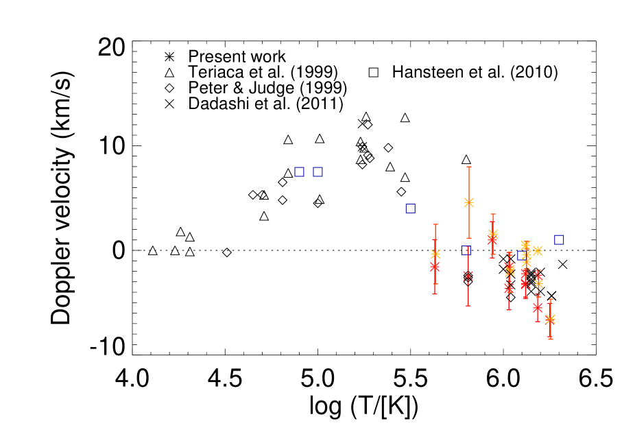
Figure 7: Radial velocity $v_{0}$ (interpretable as the Doppler shift at the disk center) as a function of the line formation temperature. Positive values indicate red shifts (downflows) while negative values indicate blue shifts (upflows). Red (orange) asterisks show the results in this study by the October (December) data. Astrerisk symbols without error bars show the results for the potentially blended emission lines Fe xi $180.40$Å and Fe xii $195.12$Å. The data points by previous observations are shown by triangles (Teriaca et al., 1999), diamonds (Peter & Judge, 1999) and crosses (Dadashi et al., 2011). Blue diamonds are the data points synthesized by using the MHD simulation results by Hansteen et al. (2010).

Obtained radial velocities $v_{0}$ from eleven emission lines for the temperature range $\log T\,[\mathrm{K}]=5.7$–$6.3$ are listed in Table 1 and these results were plotted in Figure 7. The important conclusion here is that the Doppler shifts are almost zero or slightly positive (i.e., downward) at the temperature below $\log T\,[\mathrm{K}]=6.0$, and above that temperature the emission lines are blueshifted with increasing temperature, and the Doppler shift reaches $({-7})$ – $({-6})\,\mathrm{km}\,\mathrm{s}^{-1}$ at $\log T\,[\mathrm{K}]=6.25$ (Fe xiii).

5 Discussion

To understand the dynamics in the solar transition region and lower corona, we investigated the Doppler shifts of quiet regions over a wide coronal temperature range ($\log T\,[\mathrm{K}]=5.7$–$6.3$) using the spectroscopic data taken by the Hinode EIS. By analyzing the data covering the meridian from the south to the north poles, we successfully measure the shift to an accuracy of $3\,\mathrm{km}\,\mathrm{s}^{-1}$.

Below $\log T\,[\mathrm{K}]=6.0$ the Doppler shifts are almost zero or slightly positive (i.e., downward); above this temperature, the Doppler shifts clearly become negative, reaching up to $-6\,\mathrm{km}\,\mathrm{s}^{-1}$ (see Fig. 7) . In previous observation of Ne viii $770.43$Å in the quiet region at $\log T\,[\mathrm{K}]=5.8$, the Doppler shift was measured as $-2.6\pm 2.2\,\mathrm{km}\,\mathrm{s}^{-1}$ (Peter, 1999), $-2.4\pm 1.5\,\mathrm{km}\,\mathrm{s}^{-1}$ (Peter & Judge, 1999), and $-1.9\pm 2.0\,\mathrm{km}\,\mathrm{s}^{-1}$ (Teriaca et al., 1999). Our results were in good agreement with those studies within the error margin.

Dadashi et al. (2011) measured the Doppler shift of spectral lines formed between 1 and 2 MK ( $\log T\,[\mathrm{K}]=6.0$ and 6.3, the coronal temperature range) in the quiet region see Fig. 7) . They combined the SUMER/SoHO and EIS observations around the disk center and established the absolute value at the reference temperature (1 MK) by simultaneous wavelength calibration of the SUMER spectra. They determined the velocity as $(-1.8\pm 0.6)\,\mathrm{km}\,\mathrm{s}^{-1}$ at 1 MK, peaking at $(-4.4\pm 2.2)\,\mathrm{km}\,\mathrm{s}^{-1}$ around 1.8 MK ($\log T\,[\mathrm{K}]=6.25$) , and dropping to $(-1.3\pm 2.6)\,\mathrm{km}\,\mathrm{s}^{-1}$ at 2.1 MK ($\log T\,[\mathrm{K}]=6.32$). Our results are consistent with theirs. Despite being based on different calibration methods, our study and that of Dadashi et al. (2011), commonly found a blueshift of $(-6)$–$(-4)\,\mathrm{km}\,\mathrm{s}^{-1}$, indicating a substantial upflow in the lower corona.

To explain the redshifts in the transition regions, Athay & Holzer (1982) and Roussel-Dupré & Shine (1982) conjectured the return of previously heated spicule material. Hansteen (1993) argued that redshifts arise from waves generated by nanoflares in the corona. Peter et al. (2006) reproduced the redshifts in their three-dimensional simulations although they could not clarify the mechanisms. Zacharias et al. (2011) proposed that these downflows are signatures of cooling plasma that drains from the coronal volume. Based on their comprehensive study using three-dimensional magnetohydrodynamic (MHD) models, Hansteen et al. (2010) interpreted that the pervasive redshifts in the transition regions and the weak upflows in the low corona are caused by rapid episodic heating at low heights of the upper chromosphere to coronal temperatures producing downflows in the transition region lines. Our observed near-zero Doppler shifts in the emission lines $\log T\,[\mathrm{K}]=6.0$ are consistent with the synthesized Doppler shifts in Hansteen et al. (2010) (see Fig. 7) . On the other hand, the increasing magnitude of the blueshift at higher temperature reaching $-6.3\pm 2.1\,\mathrm{km}\,\mathrm{s}^{-1}$ at $\log T\,[\mathrm{K}]=6.25$ is substantially larger than that predicted by the MHD model. This discrepancy of larger blueshifts was also observed by Dadashi et al. (2011), suggesting that the contributing solar heating events are more episodic and stronger than those presumed in Hansteen et al.’s MHD models.

For further understanding, we could investigate spatially and temporally resolved spectra. Wang et al. (2013) studied the Doppler shift in the network and internetwork regions and found enhancements of the Doppler shift magnitude and the non-thermal line width in the network regions than those in the internetwork regions. However, the physical interpretation of this difference remains unclear. In our measurements, the Doppler shifts similarly fluctuated on a scale of $100^{\prime\prime}$ by a few $\mathrm{km}\,\mathrm{s}^{-1}$. Since this spatial scale is similar but a few times larger than that of the chromospheric network, we cannot attribute this fluctuation to the network structure studied by Wang et al. (2013). Therefore, we must compare not only the detailed structures in the transition region and the corona but also the magnetic structures in the chromosphere. As stated above, previous studies and our results suggest that relatively short lived heating followed by cooling may play a major role (e.g., Hansteen et al., 2010). An effort should be made to look at Doppler shifts as a function of time over individual locations. Clearly, there are wavelength calibration issues associated with this, but if the situation is dynamic, analyzing seriously averaged data such as is done in this study may have reached the limit of its usefulness.

Our calibration procedure is modeled on the center-to-limb variation in the Doppler shift assuming that radial flows are uniformly distributed in the atmosphere at each temperature. This method, originally proposed by Peter (1999) and Peter & Judge (1999), was here improved by exploiting the spectral data in the overlapping FOV. As shown in Fig. 4 of Section 3, when the standard analysis package in SolarSoftware was applied to the EIS data, the residual error exceeded $5\,\mathrm{km}\,\mathrm{s}^{-1}$. By devising a sequential connecting procedure among neighboring pointing data, we improved the precision to better than $3\,\mathrm{km}\,\mathrm{s}^{-1}$.

Our method, although very simple, allows flexible usage of the data because it requires no reference spectrum. That is, we can analyze the EIS data without requiring simultaneous SUMER observations. On the other hand, our procedure demands a relatively large field of view covering the limb toward as further as the center. To improve the utility and reliability of our method, we need to further study its robustness. The zero-velocity assumption at and beyond the limb needs to be confirmed or limited. To quantify the fluctuation in the Doppler shift along the limb, we could analyze the observed spectral data covering the limb circle. Moreover, the applicability of the center-to-limb calibration method should be generalized from covering only the north-south meridian to coverage at any latitude. For this purpose, we must study the solar rotation in the transition region or the corona.

The results obtained in this paper will provide a reference for the Doppler shifts of outflow in active regions (Kitagawa & Yokoyama, 2015; Kitagawa, 2014; Kitagawa et al., 2010; Matsui et al., 2012; Hara et al., 2008).

Appendix A Selection of analysis lines

The emission lines analysed in this study were selected by investigating their observed profiles. In this Appendix, we describe why some emission lines are not selected for the analysis by showing each profile even though the data itself was acquired. Figure 8 shows the line profiles on the solar disk ($y=-750^{\prime\prime}$; solid line) and above the limb ($y=-1050^{\prime\prime}$; dashed line) in all EIS spectral windows of HOP79 observations taken on 2010 October 7–8. The line profiles were integrated and averaged over $100^{\prime\prime}$ spans in the solar-$y$ direction. Note that, this wider range ($100^{\prime\prime}$) than that for the Doppler analysis in the main part of this paper is chosen only for demonstrating that the rejected lines are already weak and noisy even after averaging over wider area so that they are not useful for the Doppler analysis.

Figure 8: Line profiles on the disk (solid) and off the limb (dotted). The number in the upper-left corner of each panel is the logarithmic formation temperature of the emission line. Error bars include the photon noise and the uncertainty in the CCD pedestal and dark current.

Figure 8: Continued.

He ii $256.32$Å is one of the strongest emission lines in EIS spectra and the only one with a formation temperature below $\log T\,[\mathrm{K}]=5.0$. The emission is very weak above the limb, indicating that the line originates from the bottom of the corona or lower. The solid line profile He ii $256.32$Å reveals a long enhanced red wing contributed from Si x $256.37$Å. This blending greatly complicates the analysis of He ii $256.32$Å. Ideally, the Si x can be removed by referring Si x $261.04$Å: Because both lines share the same upper transition level, this line pair has a constant intensity ratio ($I_{256.37}/I_{261.04}=1.25$; CHIANTI ver. 7, Dere et al. 1997; Landi et al. 2012). The intensity ratio could be measured above the limb, where He ii becomes much weaker than it was inside the solar disk. However, as seen from the off-limb spectrum (dotted histogram in Fig. 8) of Si x $261.04$Å, this line was too weak (i.e., noisy) to be used as a reference emission line; thus, it was excluded in the present analysis.

The analyzed EIS data include two oxygen emission lines: O iv $279.93$Å ($\log T\,[\mathrm{K}]=5.2$) and O v $248.48$Å ($\log T\,[\mathrm{K}]=5.4$). In previous reports, the transition region lines around $\log T\,[\mathrm{K}]\simeq 5.0$–$5.5$ were redshifted by up to $\sim 10\,\mathrm{km}\,\mathrm{s}^{-1}$ at the disk center (Chae et al., 1998; Peter & Judge, 1999; Teriaca et al., 1999). Therefore, to check whether our results are consistent with previous observations, we could potentially focus on these oxygen lines. Since the oxygen emission lines yield much weaker spectra than those of other observed emission lines (e.g., Fe emission lines), we integrated their spectra almost along the entire slit ($500^{\prime\prime}$) at the expense of spatial resolution. As seen from the spectra in Fig. 8, the integrating over $100$ pixels is too coarse for measuring the precise line centroid.

The emission lines Fe viii $186.60$Å and Si vii $275.35$Å are strong and well-isolated from the other strong lines; in addition, their formation temperatures are similar. A Ca xiv emission line appears near the line centroid of Fe viii $186.60$Å, but its influence is considered to be very weak in the quiet region because of the high formation temperature of Ca xiv ($\log T\,[\mathrm{K}]=6.7$). Although the formation temperature of Mg vi $268.99$Å is similar to that of Fe viii and Si vii, this line was too noisy to achieve a precision of several $\mathrm{km}\,\mathrm{s}^{-1}$; thus, it was rejected.

At the longer wavelength side in the spectral window of Fe xi $188.21$Å/$188.30$Å, there is a Fe ix $188.49$Å line, which is isolated and relatively strong. Using this line, we can fill the wide temperature gap between Fe viii ($\log T\,[\mathrm{K}]=5.69$) and Fe x ($\log T\,[\mathrm{K}]=6.04$).

There are two emission lines from Fe x in the analyzed EIS data: $184.54$Å and $257.26$Å. Neither line is significantly blended by other lines near the line center, although a weak line Fe xi $184.41$Å exists in the red wing of Fe x $184.54$Å. However, this line is much weaker than Fe x $184.54$Å in the quiet region.

Fe xi emission lines are included in three spectral windows: $180.40$Å, $188.21$Å, and $192.81$Å. Unfortunately, all of these lines are significantly blended. The line center of Fe xi $180.40$Å is very close to Fe x $180.44$Å (separation of $\sim 2$ pixels in the EIS CCD). This emission line is density-sensitive and strengthens in regions of high electron density. This strengthening may cause a systematic redshift relative to other Fe xi emission lines. The Fe xi $188.21$ line is blended with another emission line of comparative strength (Fe xi $188.21$Å/$188.30$Å; see Fig. 8). Therefore, we fitted Fe xi $188.21$Å/$188.30$Å by double Gaussians. This fitting is expected to be robust because both emission lines are strong and their line profiles usually feature two distinct peaks. The third emission line Fe xi $192.81$Å is significantly blended by the transition region lines O v $192.90$Å in the quiet region; hence, it was not used.

The emission lines Fe xii $192.39$Å and $195.12$Å are both strong and suitable for analyzing the quiet region. Unfortunately, Fe xii $195.12$Å is blended by Fe xii $195.18$Å and the line ratio $195.18$Å/$195.12$Å is sensitive to the electron density. Therefore, this emission line will shift toward longer wavelengths (i.e., redshift) as the density increases. This is especially in active regions and at bright points where the electron density is one order of magnitude higher than that in the quiet regions.

The only strong emission line from Fe xiii in our EIS study, Fe xiii $202.04$Å is recognized as a clean line with no significant blends. Different from emission lines with lower formation temperature, the off-limb spectrum of Fe xiii $202.04$Å is approximately twice as strong as the disk spectrum (see Fig. 8), as expected from the limb brightening effect.

Emission lines Fe xiv $264.78$Å and Fe xv $284.16$Å were very weak in the quiet region even after an exposure time of $120\,\mathrm{s}$. The off-limb and disk spectral behaviors of Fe xv mimics those of Fe xiii, but those of Fe xiv are very different, probably because the latter is influenced by the nearby emission line Fe xi $264.77$Å. In the quiet region, where the average temperature is lower than that in active regions, Fe xi could make a stronger contribution than Fe xiv. Fe xv might be similarly affected in the quiet region. Therefore, the Fe xiv and Fe xv emission lines were excluded as they might have yielded improper results.

References

- Athay & Holzer (1982) Athay, R. G., & Holzer, T. E. 1982, ApJ, 255, 743
- Brekke et al. (1997) Brekke, P., Hassler, D. M., & Wilhelm, K. 1997, Sol. Phys., 175, 349
- Brown et al. (2007) Brown, C. M., Hara, H., Kamio, S., et al. 2007, PASJ, 59, 865
- Chae et al. (1998) Chae, J., Yun, H. S., & Poland, A. I. 1998, ApJS, 114, 151
- Culhane et al. (2007) Culhane, J. L., Harra, L. K., James, A. M., et al. 2007, Sol. Phys., 243, 19
- Dadashi et al. (2011) Dadashi, N., Teriaca, L., & Solanki, S. K. 2011, A&A, 534, A90
- Dere et al. (1997) Dere, K. P., Landi, E., Mason, H. E., Monsignori Fossi, B. C., & Young, P. R. 1997, A&AS, 125, 149
- Doschek et al. (1976) Doschek, G. A., Bohlin, J. D., & Feldman, U. 1976, ApJL, 205, L177
- Hansteen (1993) Hansteen, V. 1993, ApJ, 402, 741
- Hansteen et al. (2010) Hansteen, V. H., Hara, H., De Pontieu, B., & Carlsson, M. 2010, ApJ, 718, 1070
- Hara et al. (2008) Hara, H., Watanabe, T., Harra, L. K., et al. 2008, ApJL, 678, L67
- Kamio et al. (2010) Kamio, S., Hara, H., Watanabe, T., Fredvik, T., & Hansteen, V. H. 2010, Sol. Phys., 266, 209
- Kitagawa (2014) Kitagawa, N. 2014, ArXiv e-prints, arXiv:1411.4742
- Kitagawa & Yokoyama (2015) Kitagawa, N., & Yokoyama, T. 2015, ApJ, 805, 97
- Kitagawa et al. (2010) Kitagawa, N., Yokoyama, T., Imada, S., & Hara, H. 2010, ApJ, 721, 744
- Kosugi et al. (2007) Kosugi, T., Matsuzaki, K., Sakao, T., et al. 2007, Sol. Phys., 243, 3
- Landi et al. (2012) Landi, E., Del Zanna, G., Young, P. R., Dere, K. P., & Mason, H. E. 2012, ApJ, 744, 99
- Matsui et al. (2012) Matsui, Y., Yokoyama, T., Kitagawa, N., & Imada, S. 2012, ApJ, 759, 15
- Peter (1999) Peter, H. 1999, ApJ, 516, 490
- Peter et al. (2006) Peter, H., Gudiksen, B. V., & Nordlund, Å. 2006, ApJ, 638, 1086
- Peter & Judge (1999) Peter, H., & Judge, P. G. 1999, ApJ, 522, 1148
- Roussel-Dupré & Shine (1982) Roussel-Dupré, D., & Shine, R. A. 1982, Sol. Phys., 77, 329
- Samain (1991) Samain, D. 1991, A&A, 244, 217
- Teriaca et al. (1999) Teriaca, L., Banerjee, D., & Doyle, J. G. 1999, A&A, 349, 636
- Wang et al. (2013) Wang, X., McIntosh, S. W., Curdt, W., et al. 2013, A&A, 557, A126
- Zacharias et al. (2011) Zacharias, P., Peter, H., & Bingert, S. 2011, A&A, 531, A97