Probing the clumping structure of Giant Molecular Clouds through the spectrum, polarisation and morphology of X-ray Reflection Nebulae

We suggest a new method for probing global properties of clump populations in Giant Molecular Clouds (GMCs) in the case where these act as X-ray reflection nebulae (XRNe), based on the study of the clumping’s overall effect on the reflected X-ray signal, in particular on the Fe K-$\alpha$ line’s shoulder. We consider the particular case of Sgr B2, one of the brightest and most massive XRN in our Galaxy. We parametrise the gas distribution inside the cloud using a simple clumping model with the slope of the clump mass function ($\alpha$), the minimum clump mass ($m_{min}$), the fraction of the cloud’s mass contained in clumps ($f_{\text{DGMF}}$), and the mass-size relation of individual clumps as free parameters, and investigate how these affect the reflected X-ray spectrum. In the case of very dense clumps, similar to those presently observed in Sgr B2, these occupy a small volume of the cloud and present a small projected area to the incoming X-ray radiation. We find that these contribute negligibly to the scattered X-rays. Clump populations with volume filling factors of $>10^{-3}$, do leave observational signatures, that are sensitive to the clump model parameters, in the reflected spectrum and polarisation. Future high-resolution X-ray observations could therefore complement the traditional optical and radio observations of these GMCs, and prove to be a powerful probe in the study of their internal structure. Finally, clumps in GMCs should be visible both as bright spots and regions of heavy absorption in high resolution X-ray observations. We therefore further study the time-evolution of the X-ray morphology, under illumination by a transient source, as a probe of the 3d distribution and column density of individual clumps by future X-ray observatories.

1 Introduction

Understanding the internal structure of giant molecular clouds (GMCs), which is driven by the interplay of turbulence, self-gravitation, and magnetic fields, is crucial when studying star formation processes in galaxies. It is, in fact, inside GMCs that dense, gravitationally unstable regions of gas, known as prestellar cores, form and collapse to give birth to stars (Williams et al. 2000).
Direct and exhaustive studies of the internal structure of GMCs are severely limited by issues of spatial and mass resolution when observing small-scale gas substructures. This is particularly true for GMCs located at a great distance, for example those found in the Central Molecular Zone (CMZ), the innermost region of the Galaxy (within $\sim$400 pc from the Galactic centre). Dense regions inside GMCs, often studied as discrete objects loosely classified as clumps and cores, span spatial ranges of 0.2-2 pc and 0.02-0.4 pc and mass ranges of $10-10^{3}M_{\sun}$ and $0.3-10^{2}M_{\sun}$, respectively (Draine 2011). At distances comparable to that from the Sun to the Galactic Center (GC), subarcsec angular resolution is therefore required for these structures to be studied in detail. Despite the challenge that such high-resolution observations pose, obtaining a clear and complete picture of the overall properties of the clump and core populations in GMCs remains a vital effort in developing theoretical models of star formation (Williams et al. 2000).
In this paper, we suggest a new method for probing global properties of the clump and core population in GMCs in the case where these act as X-ray reflection nebulae (XRNe), based on the study of their overall effect on the reflected X-ray signal.
X-ray emission from XRNe is composed both of a continuum, shaped by the interplay of scattering and absorption of the illuminating X-rays by atoms and molecules in the GMC, and by characteristic spectral features in the keV regime. The latter are caused by the emission of fluorescent photons by heavy elements following the photoionisation of tightly bound electrons by hard X-rays. The inelastic scattering of fluorescent photons down to lower energies results in a characteristic increase in the continuum at energies lower than the fluorescent features - the so called “shoudler”. This feature is most easily visible in the case of bright fluorescent lines, such as the Fe K-$\alpha$ line.
Fluorescent emission following illumination by X-rays was predicted by Sunyaev et al. (1993) in support of the claim that GMCs surrounding the Galactic Center (GC) should act as XRNe of past flares of Sgr A^∗, the super-massive black-hole located at the center of the Galaxy. If this were the case, then part of the diffuse, hard, X-ray emission observed from these GMCs should be composed of a flux in the neutral Fe fluorescent line energy (6.4 keV), caused by the imprint of past, prequiescent activity of Sgr A^∗ on the present-day (due to time delays) X-ray emission of GMCs located in its proximity. A high, time-varying flux at 6.4 keV was indeed observed in the GMC Sgr B2 by Koyama et al 1996, and has been extensively studied ever since (Murakami et al. 2000a; Muno et al. 2007; Inui et al. 2009; Ponti et al. 2010; Terrier et al. 2010; Capelli et al. 2012; Nobukawa et al. 2011; Gando Ryu et al. 2012; Clavel et al. 2013; Ponti et al. 2013; Zhang et al. 2015). Scattered flux from Sgr B2 in hard X-rays was also detected using Integral (Revnivtsev et al. 2004). Similarly, other GMCs in the CMZ (Murakami et al. 2001; Marin et al. 2015) have since been shown to act as XRNe.
Both the continuum and fluorescent spectral features of the reflected X-ray spectrum are dependent on the structure and composition of the gas itself, as well as on the properties of the X-ray source illuminating the gas, and on the relative position of the source and the gas with respect to the observer. They therefore contain a wealth of information both on the source itself and on the gas structures surrounding it.

Several models (Sunyaev & Churazov 1998; Murakami et al. 2000b; Churazov et al. 2002; Odaka et al. 2011; Marin et al. 2015) have been developed to simulate the reflection of Sgr A^∗ flares by Sgr B2, the brightest of the CMZ XRNe. These models considered different relative positions of the GMC with respect to the source, different total masses of the GMC and different density gradients of its gas.
In this work, we wish to expand on these models to investigate how more realistic models of the substructure of molecular clouds, in particular their clumpiness, would affect the reflected X-ray signal. (From now on we will refer to both clumps and cores as clumps for simplicity, as the latter term merely refers to the low-mass end of the same population of overdensities.)
In particular, we investigate the effects of the following clump population model parameters on the XRNe’s X-ray emission:

• Slope of the clump mass function ($\alpha$);

• Minimum clump mass in the clump mass function ($m_{min}$);

• Fraction of the total cloud’s mass found in clumps, or dense gas mass fraction ($f_{\text{DGMF}}$);

• The mass-size relation of individual clumps ($m=m_{norm}(r/pc)^{\gamma}$);

We use a grid-based Monte Carlo radiative transfer code in order to compute the reflected energy spectrum and polarisation of Sgr B2’s X-ray emission. In section 2 we discuss the physical processes accounted for and the Monte Carlo method used in our calculations. In section 3, we discuss the models for Sgr B2 considered, including the parameters used and the assumptions made in simulating its clump population (section 3.1). In section 4 we discuss the results obtained.

Finally, in section 5, we discuss the time-variability of the X-ray morphology of XRNe in the case of clumps, and suggest that under illumination by a non-persistent, flaring source such as Sgr A^∗, the evolution of reflected X-ray intensity can reveal information about the location of the clumps along their line of sight, and therefore on the 3d distribution of these substructures inside GMCs.

Even though we simulate the particular case of Sgr B2, our results are more generally applicable to other GMCs in the Galaxy when illuminated by other X-ray sources such as X-ray binaries.

2 Monte Carlo simulation of X-ray propagation in inhomogeneous media

In this section, we describe the physical processes accounted for in simulating the propagation of X-ray photons in neutral gas (section 2.1) and the the Monte Carlo radiative transfer code used (section 2.2).

2.1 X-ray interaction with neutral matter

X-rays interaction with atoms and molecules in the interstellar gas takes place through two processes: scattering and absorption through photoionisation.
Scattering processes of X-ray photons on bound electrons are classified as Rayleigh in the case of elastic scattering, Raman for scattering which results in the excitation of electrons in the atom or molecule, and Compton for scattering which results in the ionisation of the atom (Sunyaev & Churazov 1996). In our code, we account for these scattering processes on neutral HI, H2 and He using the results for the doubly differentiated cross-section of Vainshtein et al. (1998). The contribution of heavier elements to the total scattering cross section, for which such results are not currently available, is accounted for by approximating the interaction of X-rays with their electrons as if they were unbound.
We further include the effect of polarisation in scattering processes using the prescription of Namito et al. (1993).
Photoionisation, on the other hand, takes place through the ionisation by X-ray photons of tightly bound electrons in the atoms’ innermost shells, which results in the release of a free electron. We use cross sections from Verner & Yakovlev (1995), and include both K- and L-shell photoabsorption. The unstable electron configuration of the ionised atom prompts the filling of the K-shell vacancy by an electron in one of the higher energy levels, which causes a release of energy. This energy can either be released through the emission of a photon in the X-ray range (fluorescence) or be transferred to another electron, which is then ejected from the atom (Auger effect). The probability of either process taking place varies depending on the atomic configuration and on the original energy level of the electron that fills the K-shell vacancy. The probability of fluorescence is called the radiative yield ($Y$). In our calculation, K-shell fluorescence yields are taken from Krause et al 1979, and K_β-to-K_α ratios are taken from Ertugral et al 2007. K_α2-to-K_α1 ratios are decided by the degeneracy of $2_{p_{1/2}}$ and $2_{p_{3/2}}$ levels, which we fix to 0.5. The energies of the fluorescent lines are taken from Thompson et al 2001.
We assume a chemical composition of the Sgr B2 cloud given by a factor of 1.5 compared to protosolar abundance, as estimated by Lodders (2003).

2.2 Photon weighing method

We use a Monte Carlo grid-based radiative transfer code to simulate the propagation of X-ray photons through a cloud of complex internal structure, containing both diffuse and dense regions. We use an octree-based approach for gridding the cloud’s internal structure, which allows us to have finer grids in high density regions.
The Monte Carlo code makes use of the Pozdnyakov et al. (1983) prescription for Monte Carlo methods of X-ray propagation. This applies a weight-based approach to the radiative transfer, in which photon packages, rather than individual photons, are followed. Each package is described by a statistical weight $w$, which reflects the relative probability of photons undergoing different types of interactions, a position, $\bf{r}$, a direction of travel, $\bf{\Omega}$, and an energy, $hv$.
Photon-packages are initially emitted by the source with weight 1. Their starting position is the source’s own position, and their energy is randomly sampled from the source’s spectrum. Their initial direction is finally randomly sampled from an isotropic distribution (assuming the source radiates isotropically).
In order to compute the propagation of photon packages in our grid, we estimate at each step the relative probability of different processes occurring. A photon package $\bf{P}$, found in a given grid-cell $g$, has in fact a probability of:

• escaping the grid-cell $g$, $(L)$;

• not escaping the grid-cell $g$, $(1-L$);

and, if not escaping the grid-cell $g$, a probability of:

• being scattered, $(p_{scatt,Z})$;

• being absorbed by a K or an L shell, $(p_{abs,Z}=p_{Kion,Z}+p_{Lion,Z}$);

By considering photon packages rather than single photons, we are able to account for all the above events at once by splitting the initial photon package weight $w$ as follows:

• $w_{u}=wL$ is the probability of $\bf{P}$ crossing the grid-cell without undergoing any interaction;

• $w_{s}=w(1-L)p_{scatt,Z}$ is the probability of $\bf{P}$ undergoing a scattering event inside the grid-cell;

• $w_{fluo,Z}=w(1-L)p_{Kion,Z}Y$ is the probability of $\bf{P}$ photoionising the K shell of element $Z$ and resulting in a fluorescent emission;

We can account for these events by assigning their weight to secondary packages $\bf{P_{u}}$,$\bf{P_{s}}$, and $\bf{P_{f,Z}}$s, which will represent the relative probability of each one of those physical events taking place. Parameters $\bf{r}$, $\bf{\Omega}$ and $hv$ in $\bf{P_{u}}$,$\bf{P_{s}}$, and $\bf{P_{f,Z}}$s have, of course, to be updated, each according to the physical processes relevant for that secondary package.
Once all parameters have been updated, the calculation is iterated by taking each one of the secondary packages as an initial package $\bf{P}$, and so on for the secondary packages then produced. To limit the number of secondary photon packages that the code has to follow, we define a statistical threshold $\epsilon$ below which secondary packages are discarded.
Note that other possible events, for example the emission of an Auger electron, not listed above, as well as any secondary processes they may cause, will not result in the emission of X-ray radiation, and can therefore be safely ignored in the processing of the X-ray radiation field. They will however contribute to the deposition of X-ray energy to the interstellar gas. The convergence of the code with respect to the threshold $\epsilon$ and other parameters was verified, as well as the consistency of our results with those of Odaka et al. (2011) (for the energy spectrum) and Churazov et al. (2002) (for the polarisation spectrum).

3 Sgr B2 model

Containing $\sim$10% of the molecular mass in the CMZ, Sgr B2 is not only one of the most massive, but also one of the most complex molecular structures observed in our Galaxy. It is also one of the brightest XRNe observed, making it an ideal target for our study.
Located at a projected distance from the GC of $\sim 100$ pc, its exact position on the line of sight still remains uncertain. In a coordinate system in which the GC is located at (0,0,0), the observer at the Sun’s location (0,-8kpc, 0), and the Galactic longitude is defined in the direction of the positive $y$ axis, we assume a fixed position of the GMC at (0,100 pc,0), so that the angle between the source, the cloud and the observer is $\sim 90^{\circ}$. Discussions on how different geometries should affect the reflected X-ray signal can be found in Churazov et al. (2002) and Odaka et al. (2011).
Studies of the large scale morphology of Sgr B2 (Lis & Goldsmith 1990) show it is surrounded by a diffuse gas envelope, extending up to 22.5 pc in radius, with a near-uniform density of $n_{H2}\sim 10^{3}\text{cm}^{-3}$. What is generally referred to as the Sgr B2 cloud, and where most of the reflected X-ray signal originates, is a dense region within this envelope, of density $n_{H2}\sim 10^{4-5}\text{cm}^{-3}$ and extending out to a radius of   10 pc (Hasegawa et al. 1994). Within this region, multiple dense clumps are observed. The Sgr B2 GMC contains three well known dense clumps, named B2(N), Sgr B2(M) and Sgr B2(S). These are known to be hosting clusters of compact HII regions, providing evidence for star-formation activity within this GMC (Gordon et al. 1993). Two of these cores, SgrB2(N) and SgrB2(M) (with masses of 3313$M_{\sun}$ and 3532 $M_{\sun}$ (Qin et al. 2011) and radii 0.47 pc and 0.62 pc (Etxaluze et al. 2013) respectively), have been resolved at a subarcmin scale in X-rays (Zhang et al. 2015) and at a subarcsec scale using the Submillimeter Array (SMA) by Qin et al. (2011). The high angular resolution reached by the latter study revealed a remarkable difference in the internal structure of the two cores, with SgrB2(M) appearing to be highly fragmented to 12 sub-cores and SgrB2(N) only appearing to be divided to only 2 sub-cores, one of which contains most of the mass. The very different morphologies of the two have been speculated to be evidence in support of the idea that the two cores may represent different evolutionary stages of basically the same core, given that SgrB2(N) and SgrB2(M) are of comparable size and mass.
In our calculations, we assume Sgr B2 to have a mass of $M_{B2}=2.5\times 10^{6}M_{\sun}$ within radius 10 pc, and a diffuse H2 envelope around it as described above. In our calculations, we approximate this envelope following Odaka et al. (2011)’s prescription, by considering an initial absorption to the incoming spectrum due to a column density of $N_{H2}=6\times 10^{22}$ cm^-2. Note that this initial absorption will only affect the incoming spectrum below $\sim 4$ keV energies.
We then consider, given this mass and size, different possible models for the clump population inside the cloud, as discussed in the next section.

3.1 Simulating Sgr B2’s clump population

Statistical descriptions of the internal structure of GMCs have, since the outset of this field, been formulated in terms of discrete over-dense regions within GMCs (i.e. clumps and cores). More recently, a growing number of studies have adopted a different approach and described these density fields in terms of fractals, placing emphasis on the self-similarity of structural features at all scales (see review by Williams (1999)). In our work we will use the former approach.
The statistical study of such discrete over-dense regions has been applied to a number of nearby Galactic Plane GMCs, such as, for example, Orion and W51 (eg. Parsons et al. (2012)). This has led to the formulation of standard population properties and relations, generalised from studies of Galactic molecular clouds (eg Larson (1981)): the clump mass function (CMF) and mass-size relation of individual clumps. Such studies, along with simulations, suggest there exist similarities both in the CMF and mass-size relations between different GMCs, and therefore point towards a universal structure of GMCs in the Galactic Plane (see sections 3.1.2 and 1). The internal structure of GMCs in the CMZ, on the other hand, is likely to greatly differ from that observed in Galactic Plane GMCs, due to the extreme environment (both in density (Lis & Goldsmith 1990) and pressure (Kruijssen et al. 2014)). Understanding how the clump population of these objects differs from the ones found in Galactic Plane GMCs, would, therefore, give an important insight into how environmental factors affect the process of internal structure formation.
As previously discussed, such studies for GMCs in the CMZ are rather more difficult to perform, due to the large distance and mass of these complexes: catalogs of clump and core populations in these GMCs are known to be incomplete, and therefore don’t allow for a reliable estimate of their statistical properties.
In our calculations, we consider different possible shapes of the CMF and mass-size relation (see sections 3.1.2 and 1 respectively). We also consider different levels of fragmentation of the cloud into clumps by considering different possible values of the dense gas mass fraction, or the fraction of the cloud’s mass found in clumps, $f_{\text{DGMF}}$ (see Fig. 1).
The simulation of different clump population models for Sgr B2 is then performed as follows: given a $f_{\text{DGMF}}$ and CMF, we sample the clumps’ masses from the CMF in the mass range $m_{min}-m_{max}$, with $m_{max}=10^{4}$ M_☉, until we have obtained a total mass of $M_{DGMF}\sim f_{\text{DGMF}}\times M_{B2}$. We then proceed to assign each clump with a size based on its mass assuming a mass-size relation. Finally, we uniformly distribute the resulting clumps inside the cloud, and calculate the interclump density using the ”left-over” mass, $M_{interclump}\sim(1-f_{\text{DGMF}})\times M_{B2}$ and the ”empty” (i.e. not occupied by clumps) volume, assuming the interclump density is homogeneously distributed.
In the following sections, we discuss the details of this procedure, together with the range of parameters considered and the assumptions made in doing so.

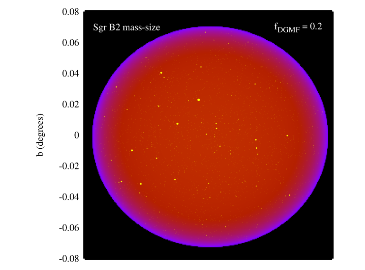
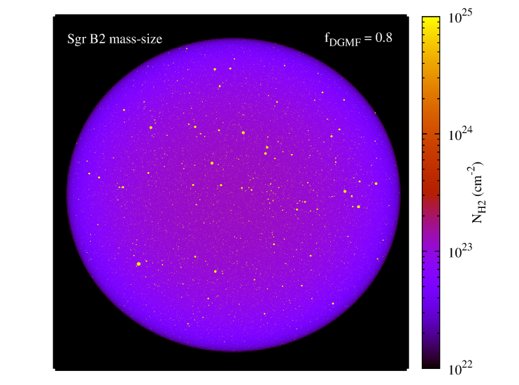
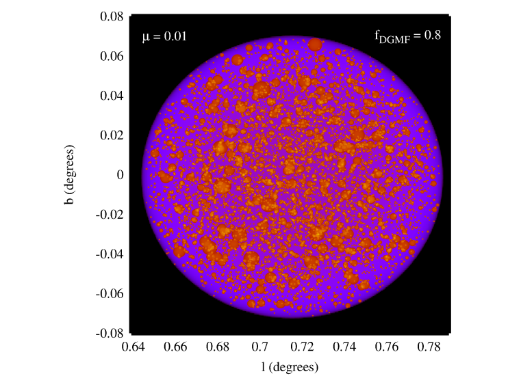
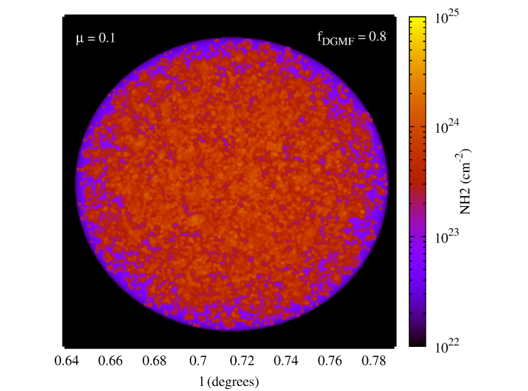
Figure 1: Cumulative column density ($N_{\text{H2}}$) along line of sights, excluding ISM and diffuse envelope contributions. The maps show Sgr B2 models with fixed parameters $\alpha=1.35$, $m_{min}=10M_{\sun}$ and Sgr B2 mass-size relation, and two values of $f_{\text{DGMF}}$. The concentration of mass into small dense regions reduces the interclump density, as seen from the figures. For the case of $f_{\text{DGMF}}=0.8$, we also show clump populations with mass-size relations tuned to obtain a volume filling fraction of $\mu=0.01$ and $\mu=0.1$.

3.1.1 Clump Mass Function

The clump mass function (CMF) of clump populations observed in Galactic plane GMCs takes the following form (McKee & Ostriker 2007):

$$m\frac{\text{d}N}{\text{d}m}\propto m^{-\alpha}$$ (1)

The slope of the clump mass function is similar to that for GMCs as a whole, possibly because both are determined by turbulent processes within larger, gravitationally bound systems (McKee & Ostriker 2007). The parameter $\alpha$ takes different values in different mass ranges. The low mass end of the function is known as the core mass function. Its shape is particularly important in relation to the Initial Mass Function (IMF) of stellar populations (McKee & Ostriker 2007). Evidence of similarity in the core mass function with the IMF were first studied by Nutter & Ward-Thompson (2007) in the Orion complex, which for the first time observed a turnover at $\sim 1.3M_{\sun}$, which mimics the turnover seen in the stellar IMF at  0.1 $M_{\sun}$. Fitting the data with a three part power law function similar to that observed in the stellar IMF:

$$\alpha=\begin{cases}-0.3&\mbox{if }0.4M_{\sun}<m<1.3M_{\sun}\\ 0.3&\mbox{if }1.3M_{\sun}\leq m\leq 2.4M_{\sun}\\ 1.35&\mbox{if }m>2.4M_{\sun}\end{cases}$$ (2)

for clump mass ranges below 100$M_{\sun}$. The physical significance of the turnover mass is not clear, as the same work highlights that similar studies in the lower-mass and nearer cloud complex $\rho$ Ophiuchi showed no turnover in their CMF ((Motte et al. 1998)). Later studies on the low-mass end of the CMF in the Aquila rift cloud complex also confirmed a variation in this parameter: Könyves et al. (2010) found a turnover mass of $\sim 0.6M_{\sun}$ in the starless core sample, and $\sim 0.9M_{\sun}$ prestellar (starless and gravitationally bound) sub-sample.
The similarity of the CMF with the Salpeter (1955) stellar IMF has been further confirmed in higher mass ranges by Tsuboi & Miyazaki (2012) (range ¿ 900 $M_{\sun}$) and Parsons et al. (2012) (range ¿ 200 $M_{\sun}$).
Despite the fact that the CMF appears to be consistent throughout Galactic Plane GMCs, the extreme environment of Sgr B2, as previously discussed, suggests the CMF for this GMC could be significantly different. Unfortunately, because of a lack of exhaustive data, how this function should differ is not obvious. We therefore adopt the Nutter & Ward-Thompson (2007) three-part power law fitting, but consider different $\alpha$ values in the highest mass interval. In particular, we consider $\alpha=1.35$ (i.e. Galactic Plane value)$,1,0.5,1.8$ (see Fig. 2). We sample this range up to clump masses $10^{4}M_{\sun}$, to be consistent with the observed massive cores in Sgr B2 (eg Qin et al. (2011)). We maintain the low-mass threshold of the CMF as a parameter in the model, $m_{min}$, and investigate its effect on the reflected X-ray signal.

Figure 2: Clump mass functions for different $\alpha$ with $f_{\text{DGMF}}=0.4$. The grey solid lines show the distributions sampled, while the coloured lines show the actual realisation. The vertical lines show the values at which the CMF changes in slope.

3.1.2 Clumps mass-size relation

The mass-size relation of individual clumps is particularly important for our study, as it determines the volume filling fraction, $\mu$, of the clump population given its $\alpha$, $m_{min}$ and $f_{\text{DGMF}}$ parameters. The volume filling fraction in return determines how effectively clumps ”hide” part of the cloud’s mass, by concentrating it into small volumes which X-rays have a low probability of intercepting.
For clumps formed inside GMCs via turbulent fragmentation, one would expect a mass-density, or similarly a mass-size, relation (Donkov et al. 2011). A first suggestion of this relation based on observations was formulated in the seminal paper of Larson (1981), which claimed a universal power-law mass-size relationship should describe all clouds and clumps found in the Galaxy. This is commonly referred to as ”Larson’s third law”, and it suggested that the relation should go as:

$$m=m_{norm}r^{\gamma}$$ (3)

with $\gamma=2$. Since being first formulated, this empirical observation has been extensively studied both in observations (eg Kauffmann et al. (2010); Lombardi et al. (2010)) and in simulations (Shetty et al. 2010; Donkov et al. 2011), which all find a deviation from the power of 2 originally found by Larson (1981). The latter two find that on scales $<1$pc, the mass size relation studied in eleven different GMC structures in the Galactic Plane, can be described as $m(r)=400M_{\sun}(r/pc)^{1.7}$ and $m(r)=380M_{\sun}(r/pc)^{1.6}$ respectively. By looking at these clouds individually, Lombardi et al. (2010) find that these clouds have quite similar exponents, but rather different normalisation masses (ranging from 170 to 710 $M_{\sun}$).
Although such studies haven’t been performed for the clump population of Sgr B2, we can use observational data currently available to get a rough estimate of what this relation should look like for this GMC.
We use the data available from the 14 cores within Sgr B2(N) and SgrB2(M) resolved in the subarsec observations of Qin et al. (2011) (see section 3) to infer a mass-size relation for Sgr B2. Assuming a homogeneous density distribution inside the clumps, we fit the power law to these observations and find:

$$m(r)=4.68\times 10^{5}M_{\sun}(r/pc)^{1.77}$$ (4)

which we refer to here-forth as the ”Sgr B2 mass-size relation”. We see that the exponent is consistent with the results of Lombardi et al. (2010), but that the normalisation mass is considerably higher. This is somehow expected, considering that the average density in Sgr B2 is considerably higher than that found in Galactic plane GMCs. Note that the range of sizes of these cores is considerably below the Lombardi et al. (2010) range. In our model, we assume this relation, inferred in a somewhat limited mass range, holds for all possible clump masses.
As already mentioned, the mass-size relation is particularly important for our study as it effectively determines the volume filling factor of a given population. The volume filling factor, $\mu$, can be expressed in terms of other clump population parameters as follows:

$$\mu=\frac{4\pi}{3V_{SgrB2}}\frac{C}{m_{norm}^{3/\gamma}}\frac{[m^{-{\alpha}+3/\gamma}]^{m_{max}}_{m_{min}}}{-{\alpha}+3/\gamma}$$ (5)

where

$$C=\begin{cases}M_{DGMF}(1-\alpha)([m^{-\alpha+1}]^{m_{max}}_{m_{min}})^{-1}&\mbox{if }\alpha\neq 1\\ M_{DGMF}[\text{ln}m]^{m_{max}}_{m_{min}}&\mbox{if }\alpha=1\end{cases}$$ (6)

Using equation 5, and assuming the mass-size relation given in Eqn. 4, we obtain a maximum filling fraction, among all $f_{\text{DGMF}},\alpha$ and $m_{min}$ values considered, of only $10^{-4}$ (see Fig. 3). Therefore the probability of X-rays intercepting the clumps will be extremely low. Hence, we don’t expect parameters related to the mass distribution of the clumps, i.e. $\alpha$ and $m_{min}$, to significantly affect the X-ray signal when assuming this mass-size relation. We will also consider how the X-ray signal should be affected by increasingly large values of $\mu$, by varying the $m_{norm}$ value in the mass-size relation accordingly (see section 4.2).
The mass-size relation can be alternatively expressed as a column density-mass relation to the center of the cloud. Defining $\tau_{\text{H2}}=rn_{\text{H2}}\sigma$, this takes the following form:

$$\tau_{\text{H2}}=m_{norm}^{2/\gamma}\frac{3\sigma}{m4\pi}m^{-2/\gamma+1}$$ (7)

The effect of the mass-size relation on the clumps’ contribution to the column density of the GMC is shown in Fig. 1.

Figure 3: Normalisation parameter $m_{norm}$ in the mass-size relation as a function of the volume filling factor $\mu$, calculated using Eqn. 5, for different $f_{\text{DGMF}}$ at fixed $\alpha=1.35$, $m_{min}=100M_{\sun}$ and $\gamma=1.77$. We also show the $\mu$ values obtained using the fixed Sgr B2 relation. Note that for high $\mu$ and low $f_{\text{DGMF}}$ values, we obtain mass-size relations yielding clump populations where the least dense clump, given by the clump with the highest mass ($m_{max}$), is less dense than the interclump density $n_{interclump}$, in contradiction with the very definition of clump as an overdensity; we clearly mark these models in red in the plot. We will use the $f_{\text{DGMF}}$ value that allows us to explore a widest possible range of $\mu$, $f_{\text{DGMF}}=0.8$, to investigate the impact of increasing $\mu$ on the reflected X-ray signal (see Fig. 7).

3.1.3 Dense gas mass fraction

Studies of this parameter in Galactic GMCs, as for example in W51 (Battisti & Heyer 2014; Ginsburg et al. 2015), show a variety of possible stages of fragmentation in different clouds, reflecting the different evolutionary stages GMCs are found in. We therefore span a wide range of $f_{\text{DGMF}}$ values: $f_{\text{DGMF}}=0.2,0.4,0.6$ and 0.8.

3.1.4 Spatial distribution of clumps

In our model we assume clumps are not overlapping and are isotropically distributed inside the cloud.
The latter assumption is a clear simplification of what is currently being observed in CMZ GMCs (eg Chen & Ostriker (2015)). In the case of very low volume filling factors, as in the case of clumps following the Sgr B2 mass-size relation, this assumption should have a negligible effect on the reflected signal. In the case of larger volume filling factors, on the other hand, this may become relevant. The percolation of the X-ray photons will be dependent on the projected area filling on the plane perpendicular to the source-cloud direction, rather than on the volume filling factor itself. The maximum possible projected area occupied by the clumps, in the case where no line of sight from the source intercepts more than one clump, is $\propto\pi\sum_{i=1}^{N}v_{i}^{2/3}$, where $v_{i}$ is the volume of the single clump $i$. The minimum possible project area on the other hand, in the case where all clumps are centered along a single line of sight, is $\propto\pi v(r_{max})^{2/3}$, where $v(r_{max})$ is the volume of the largest clump in the population. The actual value of the projected area occupied by the clumps will be somewhere between these two extremes, and will be determined by the distribution of the clumps inside the cloud. We postpone an investigation of how the spatial distribution of discrete over-dense regions affects the reflected X-ray signal to a later study.

4 Results

We consider a persistent Sgr A^∗ flare of luminosity $1.3\times 10^{39}$ erg/s, modeled with a power law photon index of 1.8 and assumed to be completely unpolarised. For each model considered, we plot the energy spectrum and polarisation fraction of the reflected X-ray emission. The polarisation fraction is calculated as the fraction of the Stokes Q parameter (with the frame of reference chosen so that U=0) intensity over the total intensity reaching the observer.
First, we consider the case where the mass-size relation of the clumps is the Sgr B2 relation discussed in section 3.1.2. We then consider, for fixed $f_{\text{DGMF}},\alpha$ and $m_{min}$ parameters, the effect of varying the normalisation of the mass-size relation, and therefore the volume filling factor of the clump population, on the reflected signal.

4.1 Fixed Sgr B2 mass-size relation

We consider a fiducial model given by $f_{\text{DGMF}}=0.4,m_{min}=10M_{\sun},\alpha=1.35$, and vary each parameter individually around it while maintaining the mass-size relationship constant at $m_{norm}=4.68\times 10^{5}M_{\sun}$ and $\gamma=1.77$ according to Eqn. 4.

Figure 4: Reflected energy spectrum and polarisation fraction for varying $f_{\text{DGMF}}$ cloud models. The energy spectrum is shown with resolution of 20 eV.

Figure 5: Reflected energy spectrum and polarisation around the 6.4 keV Fe K-$\alpha$ line for varying $f_{\text{DGMF}}$. The spectral resolution is 5 eV. The rightmost panel shows the ratio of EW for the 6.4 keV shoulder to the line.

In Fig. 4, we compare the reflected X-ray emission for different values of the fragmentation parameter $f_{\text{DGMF}}$. For all models considered, we observe that an increase in the fragmentation level of the cloud into clumps results in: a slight increase in the flux of low energy photons, a decrease in the flux of higher energy photons, and a decrease in the Fe shoulder’s flux (see Fig. 5).

These three effects can all be accounted for by considering percolation: because the probability of intercepting the clumps will be extremely low, due to the small ($<10^{-4}$) volume filling fraction of the clumps, the X-ray photons will mainly interact with the atoms and molecules in the interclump medium. The resulting reflected spectra will therefore be consistent with those resulting from reflection off homogeneous clouds with the same size, and density equal to the interclump density. In Fig. 6 we compare the X-ray emission obtained from cloud models where a fraction $f_{\text{DGMF}}$ of the total cloud’s mass is found in clumps and homogeneous cloud models with a total mass of $M_{B2}\times(1-f_{\text{DGMF}})$. We find indeed that the fractional difference between the two cases is negligible for all energies, and that the $f_{\text{DGMF}}=0.2,0.4,0.6$ and $0.8$ models can be approximated by homogeneous clouds with $\tau_{\text{HI}}\sim 0.32,0.24,0.16$ and 0.08 respectively (where $\tau=R\times n_{\text{HI}}\times\sigma_{Thoms}$).

The decrease in the number of scatterings due to an increase in the dense gas mass fraction can also be observed in the plots of the polarisation fraction of the reflected spectra (Fig. 4). An analytic approximation to the polarisation fraction of an X-ray photon undergoing $n$ scatterings is given by (Churazov et al. 2002):

$$P_{n}=\frac{1-\eta^{2}}{1+\eta^{2}+\frac{20}{15}\big{(}\big{(}\frac{10}{7})^{n-1}-1\big{)}}$$ (8)

where $\eta=cos(\theta)$ and $\theta$ is the average scattering angle. From this analytic prescription, it is indeed for the geometry considered in these calculations, the polarisation fraction should be close to unity for singly scattered photons, in the case of scattering close to  90^∘ as is the case here, as and should progressively decrease from unity as the number of scatterings increases. With increasing energy the absorption optical depth decreases and the relative contribution to the radiation escaping from the cloud from multiple scatterings increases. This is evident in Fig. 4 as decrease in degree of polarisation with increasing energy.

In Fig. 4, we can clearly see that the polarisation fraction of the shoulder progressively increases with the dense gas mass fraction. This means that the higher the fraction of the cloud’s gas found in dense regions, the lower the number of multiple scatterings photons experience, in agreement with a picture of an increasing rate of percolation. Fluorescent photons, on the other hand, are emitted isotropically by photoionised atoms, and therefore are completely unpolarised. For varying $\alpha$ and $m_{min}$ parameters we find that, on the other hand, these have no effect on the overall reflected signal. This reinforces the idea that the dominant effect of clumping within the XRN (in the case of the Sgr B2 mass-size relation) is percolation, and that the mass concentrated in clumps is effectively ”hidden” from incoming X-ray photons because of the small volume it occupies.

Figure 6: Fractional difference between the reflected energy spectrum for a cloud model with mass $M_{B2}$ and a fraction $f_{\text{DGMF}}$ of its mass found in clumps and a homogeneous cloud model with total mass $M_{B2}\times(1-f_{\text{DGMF}})$. The fractional difference is negligible for all energies, reinforcing the idea that the clumping of part of the cloud’s mass into very dense region effectively ”hides” that mass from the incoming X-rays.

4.2 Variable mass-size relation

The picture painted in section 4.1 of course only holds if the volume filling fraction of the clump population is low enough to effectively reduce the probability of interaction between photons and overdensities to a negligible value. Should the volume filling fraction increase, as would result from a variation in the mass-size relation of the clumps (see section 3.1.2), then X-rays should start intercepting the clumps at a more significant rate, with consequences to the reflected spectrum.
In particular, an increase in the absorption probability should result in an increase in the fluorescent lines, while an increase in the scattering probability should result in an increase in the fraction of fluorescent photons scattered, and therefore of the fluorescent line’s shoulder’s flux. In Fig. 7, we show the energy and polarisation spectrum around the 6.4 keV K-$\alpha$ line for cases of increasing high volume filling factor. We find that, as expected, both the line and the shoulder’s flux increase with increasing $\mu$.
Once the probability of intercepting clumps increases, we expect properties of the clump populations such as $m_{min}$ and $\alpha$ to play a more significant role in shaping the reflected X-ray signal. In Fig. 8, we compare, for fixed $\mu=0.01$, the reflected signal in the case of varying $\alpha$ and $m_{min}$ parameters respectively. Indeed, we observe that already for this volume filling fraction the slope shows a dependence on the two population parameters: a higher CMF slope will result in a higher number of clumps with larger masses (and hence radii) being selected. Because these are more likely to intercept the incident X-rays, we expect an increase in the Fe shoulder’s flux in correspondence with increasing $\alpha$, as it is indeed observed in the figure. A decrease in $m_{min}$ puts more mass in smaller clumps, resulting in a decrease in the fluorescent lines and shoulders in Fig. 8. However, a photon which is emitted inside a denser clump is also more likely to be scattered before it escapes, and therefore the ratio of the shoulder to line increases with decreasing $m_{min}$, as seen in the EW ratio plot in the same figure.

Figure 7: Reflected energy (top plot) and polarisation (bottom plot) around the 6.4 keV Fe K-$\alpha$ line for varying $\mu$, shown with resolution of 5 eV. Values of $\mu$ illustrated were obtained by adjusting the $m_{norm}$ parameter in the mass-relation of clumps using Eqn. 5. As expected, for increasingly large volume filling factors, the probability of fluorescent photons intercepting the clumps increases, resulting in an increase in the shoulder’s flux. Note that, because the X-ray signal is really dependent on the projected area (see section 3.1.4), which roughly goes as $\mu^{2/3}$, we would expect a volume filling factor of $\mu\sim 0.001$ (project area $\sim 0.01$) to already produce a visible signature in the X-ray spectrum. Indeed, from the polarisation fraction plot, it is clearly visible that at $\mu=0.001$ the signal starts deviating from the virtually homogeneous case.

Figure 8: Reflected energy (left plots) and polarisation (centre plots) around the 6.4 keV Fe K-$\alpha$ line (shown with resolution of 5 eV) and shoulder to line ratio (right plots) for varying $\alpha$ (top plots) and $m_{min}$ (bottom plots) parameters at fixed $\mu=0.01$. Values of $\mu$ illustrated were obtained by adjusting the $m_{norm}$ parameter in the mass-relation of clumps using Eqn. 5. For increasing $\alpha$, we expect an increase in the number of clumps being sampled from the higher mass range, resulting in a greater average size of the clumps in the population. In return, this results in an increase in the probability of X-rays intercepting them. Indeed, an increase in the Fe shoulder for increasing $\alpha$ is observed both in the energy and polarisation spectrum. The fragmentation of the clumps to lower and lower $m_{min}$, on the other hand, results in a larger projected area of the clump population, which increases the probability of interaction with incoming X-rays. This effect in also observed in the plots.

5 Time-evolution of the XRN morphology as a probe of the 3d distribution of substructures

Figure 9: Schematic representation (not to scale) of parameters used in Eqn. 9

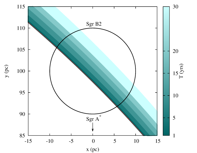
Figure 10: Top plot: Regions of the x-y plane visible to the observer at different times through scattered X-ray photons, in the case of photons originally emitted by an instantaneous flare of Sgr A^∗ (i.e. all photons emitted at $t=0$). Bottom plot: Regions of the x-y plane visible to the observer through scattered X-rays at time $t=320$ yrs in the case of an instantaneous flare (dashed line) and in the case of flares of duration $T$ (coloured maps). The longer the duration of the flare, the thicker the region of the sky observable simultaneously.

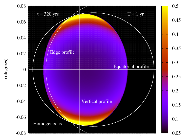
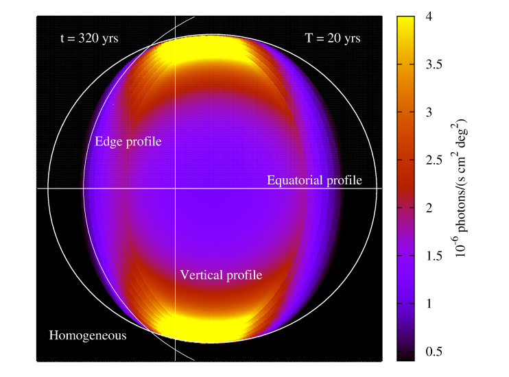
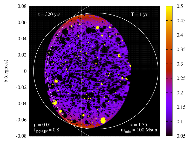
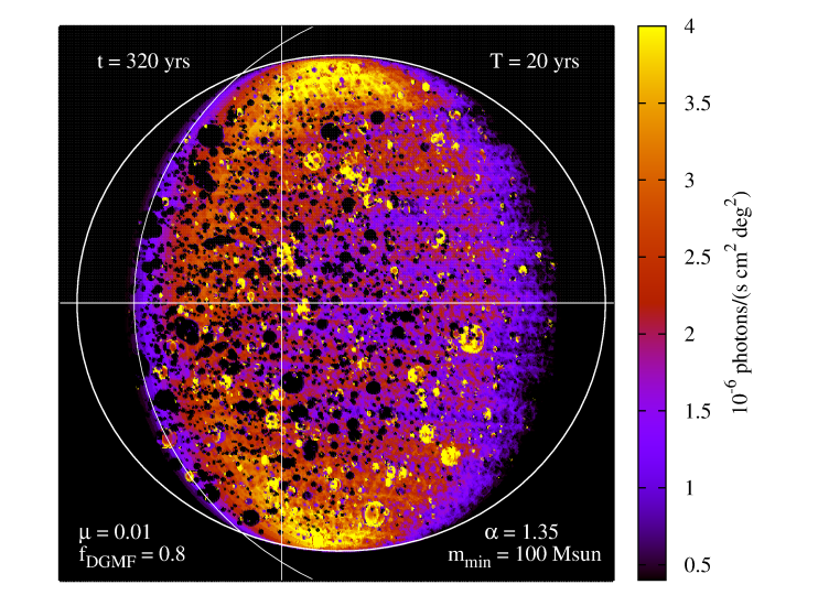
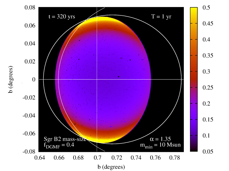
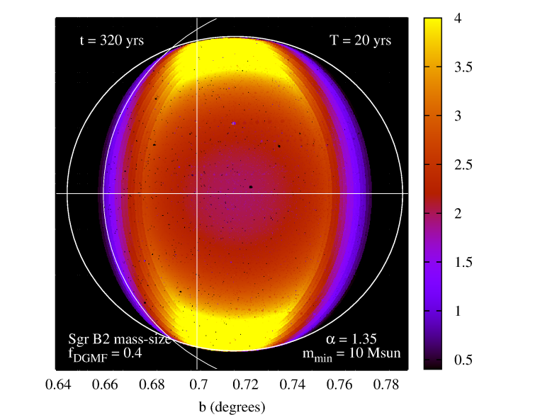
Figure 11: Analytic, single scattering approximation of the 3-20keV reflected X-ray intensity observed at time $t=320$ yrs for the three cloud models discussed in the text, and for the case of a short (1 yr) and long (20 yr) flare. The angular resolution used is of 1 arcsec. The intensity and column density profiles for the equatorial, vertical and edge profiles indicated in the maps are shown in Figs. 12 and 13 respectively.

Figure 12: Scattered intensity profiles for the homogeneous and $\mu=0.01$ model for the $T=1$ yr (thick lines) and $T=20$ yrs (thin lines).

Figure 13: Column density from the source to the point of scattering (darker colours) and from the point of scattering to the observer (lighter colours) along profiles indicated in Fig. 11, excluding the contribution of the diffuse envelope. The plots show the case of minimum column density ($t^{\prime}=0$) at time $t=320$ yrs. The different mass-size relations assumed in clump models ”Sgr B2 mass-size” and ”$\mu=0.01$” result in the latter case presenting: a higher probability of intercepting clumps, broader absorption features in the intensity profiles, and lower column density peaks.

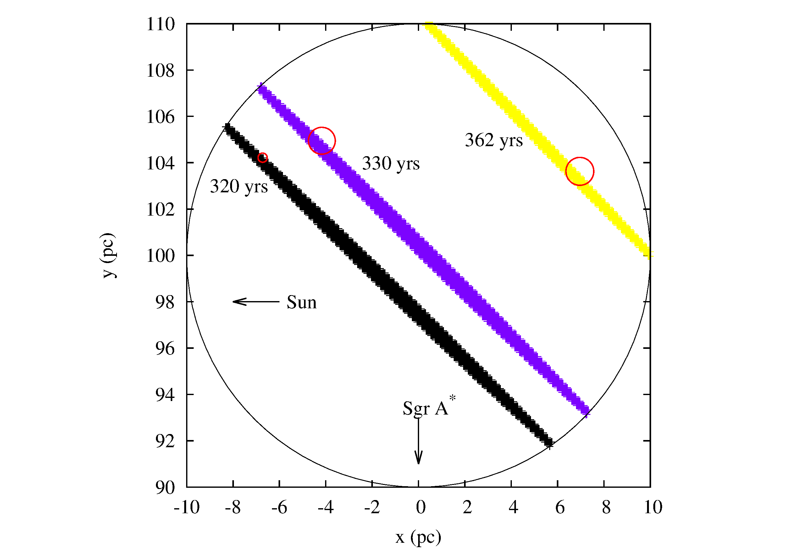
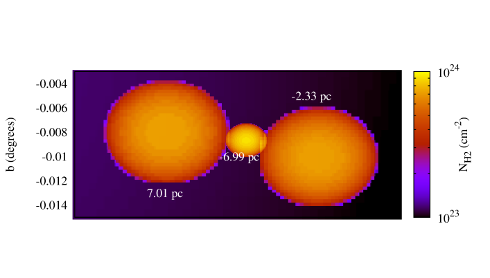
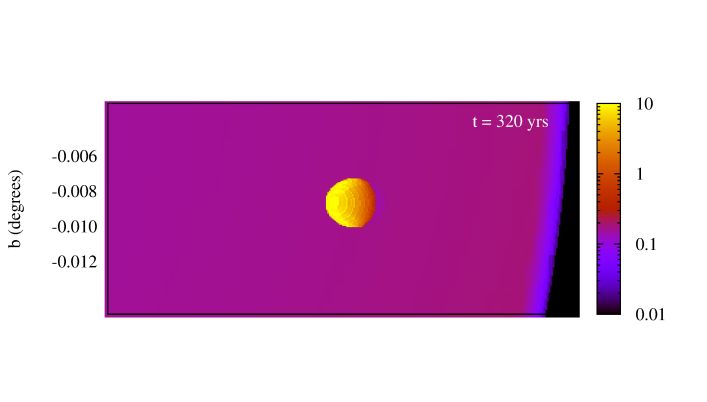
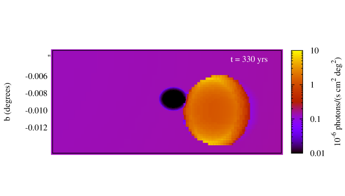
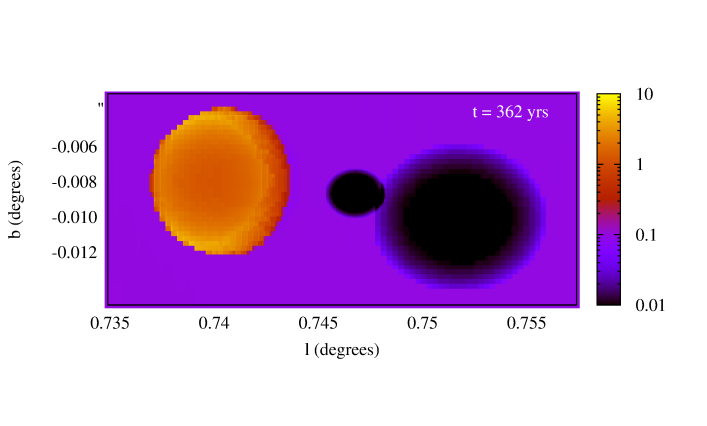
Figure 14: Top plot: Column density map of three simulated clumps within Sgr B2, found in a small region of the sky (labels in plot indicate the clumps’ distance from the center of the cloud, approximated as $D-D_{\text{SgrB2}}$). Second plot: projected location of the clumps inside Sgr B2 and regions inside Sgr B2 visible to the observer at times when the substructures should become visible (assuming illumination by an instantaneous flare). Third, fourth and fifth plot: reflected X-ray intensity reaching the observer at different times. Despite the apparent proximity of the clumps on the sky, because of the different distance at which they are located along the line of sight, the clumps are visible through their reflected X-ray emission at different times, so that when one is visible, the others are not.

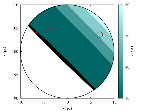
Figure 15: Projected regions inside the cloud observed simultaneously at time 320 yrs by flares of different durations $T$ (where the black region corresponds to illumination by an instantaneous flare). In the case of the three clumps considered in Fig. 14, the minimum flare duration required for the two most further apart clumps (shown with solid red lines in the plot) to both be visible to the observer at the same time is $T\sim 40$ yrs. In the case in which both substructures are visible simultaneously in the reflected X-ray intensity maps, one can infer that the source’s flare must have lasted at least $T\sim 40$ yrs.

Due to the finite speed of light, illumination by a flare of duration shorter than the light-crossing time of the cloud results in different regions of the GMC being visible to the observer, in the form of reflected X-ray emission, at different times. The evolution of the reflected X-ray intensity, therefore, acts as a scan of the density structure of the cloud as the wavefront propagates through it (Sunyaev & Churazov 1998). In this section we discuss the importance of this effect in the context of the study of the GMC’s clumps properties and distribution.

For these calculations we focus on three of the Sgr B2 models considered in the previous sections:

• the fiducial model, which assumes parameters $f_{\text{DGMF}}=0.4$, $m_{min}=10M_{\sun}$, $\alpha=1.35$ and the Sgr B2 mass-size relation consistent with observations of real Sgr B2 clumps (see section 3.1.2). We refer to this model as the ”Sgr B2 mass-size” model;

• the homogeneous model, where we assume no clumps at all;

• a more “visible” clump population model, which considers a case in which most of the gas ($f_{\text{DGMF}}=0.8$) is contained in relatively massive ($m_{min}=100M_{\sun}$) clumps, which are described by a mass-size relation constrained to obtain a volume filling fraction as large as $\mu=0.01$ (see section 3.1.2). This case ensures clumps will be numerous and voluminous enough to be easily recognisable in our calculations. We refer to this model as the ”$\mu=0.01$” model;

While these calculations were being performed, NuSTAR was able to resolve the Sgr B2 clumps Sgr B2(N) and Sgr B2(M) in X-rays for the first time (Zhang et al. 2015). This new result shows the feasibility and potential that high-resolution studies of the X-ray morphology of GMCs in the CMZ have in the study of the internal structure of these XRNe. We stress, however, that the mass-size relation assumed in our Sgr B2 mass-size model makes use of the Qin et al. (2011) observations of the clumps, which were able to resolve the Sgr B2(N) and Sgr B2(M) clumps into distinct and independent substructures. The clumps for this model obtained in our simulation will therefore be more compact than the region of gas considered by the Zhang et al. (2015) observations.

In a single scattering approximation, the distance $D$ along the line of sight $(l,b)$ at which light has to be scattered in order to reach the observer at time $t$, defined such that $t=0$ is the time at which the flare was last observed directly, is given by:

$$D(t,t^{\prime})=\frac{ct^{2}-O_{x}^{2}+2ct(|O_{x}|-t^{\prime}c)+(|Ox|-t^{\prime}c)^{2}}{2(ct+(|O_{x}|-t^{\prime}c)+O_{x}\text{cos}(b)\text{cos}(l))}$$ (9)

where $O_{x}=-8$ kpc is the Sun’s location with respect to the emitting source (assuming $O_{y}=O_{z}=0$), and $-T\leq t^{\prime}\leq 0$ is the time during the flare of duration $T$ at which the photon was emitted, as illustrated in Fig. 9. The region illuminated at a given time is therefore an ellipsoid, with its focus at the observer’s position. For the case of an observer located at the Sun’s position, this can be approximated, in the proximity of Sgr B2, by a paraboloid (Cramphorn & Sunyaev 2002). The propagation of the section of the ellipsoid on the x-y plane is illustrated, for the case of an instantaneous flare ($T=0$), in Fig. 10.

In the case of a flare with finite duration, that is $T>0$, the duration of the flare determines the “thickness” of the ellipsoid, or in other words the thickness of the region simultaneously visible to the observer, as illustrated in Fig. 10. The surface brightness observed along a line of sight at a given moment, $I(l,b,t)$, will therefore be determined not by the total optical depth of the cloud in that direction, but rather by the surface density in the section of the cloud delimited by the thick paraboloid (Sunyaev & Churazov 1998), whose boundaries are determined by the beginning and end of the flare. The reflected intensity can therefore be described, under a single scattering approximation, as:

$$I(l,b,t,\nu)=\int_{-T}^{0}\sum_{Z}\frac{\rho(\nu)}{4\pi R^{2}}n_{Z}\frac{\text{d}\sigma_{Z}}{\text{d}\Omega}\text{exp}(-\tau_{Z})c\text{d}t^{\prime}$$ (10)

where $\rho(\nu)$ is the number of photons/(s keV) emitted by the source, $R$ is the distance from the source to the point of scattering, $n_{z}$ is the density at the point of scattering, $\frac{\text{d}\sigma_{Z}}{\text{d}\Omega}$ is the singly-differentiated cross section, computed using the public library xraylib (Schoonjans et al. 2011) and:

$$\tau_{Z}=\text{NHI}(\sigma_{abs,Z}+\sigma_{scatt,Z})$$ (11)

is the total optical depth, from the point of emission to the point of observation. In $\sigma_{scatt}$ we only consider the Raman and Compton scattering cross section, since Rayleigh scattering mainly contributes towards scattering at small angles, and therefore will have a negligible effect towards scattering photons out of the path traveled.

Due to their higher average density, clumps are able to contribute significantly towards $I$, by scattering more X-ray flux towards the observer compared to the interclump medium, and hence should be clearly recognisable in the morphology of the XRN at times when they are intercepted by the propagating paraboloid, as first suggested by Sunyaev & Churazov (1998). Once the paraboloid has passed them, the clumps should significantly contribute towards the intervening column density NHI, and therefore still be visible in the morphology of the XRN as regions of absorption.

In Fig. 11, we illustrate this in the case of the three clump models described at the beginning of the section, both in the case of a short ($T=1$ yr) and longer ($T=20$ yr) flare, in a snapshot at time $t=320$ yr. The intensity and column density for the equatorial, vertical and edge profiles indicated on the maps are shown in Figs. 12 and 13 respectively.

In the maps, the main visible effects are the following:

• the contribution of clumps towards the scattered intensity is indeed clearly visible in the form of bright spots, consistently with the findings of Zhang et al. (2015);

• intervening clumps located between the source and the point of scattering, or between the point of scattering and the observer (see Fig. 13) considerably contribute to the absorption of the X-ray radiation, and are therefore observable as regions of absorption in the maps;

• The effect of the duration of the flare is also recognisable: the longer the duration of the flare, the thicker the region of the cloud probed by the ellipsoid at the same time, hence the higher the number of clumps probed by the paraboloid simultaneously, as clearly seen in the $\mu=0.01$ model maps.

• In the case of clumps with Sgr B2 mss-size relation, the very small volume they occupy means the probability of a short flare intercepting them is very low, and in fact very few clumps are intercepted at all for this particular distribution, and most clumps are therefore only seen in absoprtion;

• the intensity of the interclump regions in the Sgr B2 mass-size model (average density $n_{H2}\sim 1\times 10^{3}$ cm^-3), is higher than that of the homogeneous model (average density $n_{H2}\sim 1\times 10^{4}$ cm^-3) in the central region of the cloud. This is due to the fact that, although contributing a larger surface density within the thick paraboloid, the homogeneous cloud also results in a larger absorbing column density, as shown in Fig. 13;

The reflected intensity at a given time can therefore reveal information on the column density of both the clump and the interclump medium. But it also contains information on the distribution of the clumps inside the cloud.

In the case of a short flare, the distance along the line of sight observed at a given time is uniquely defined by the time of observation, since $D(t,t^{\prime})\sim D(t,t^{\prime}=0)$. In this case, by comparing the time at which a clump becomes visible on the reflected intensity map with its location on the sky, it is possible to constrain its position $D$ along the line of sight, as illustrated in Fig. 14. This kind of analysis could therefore prove to be important in the study of the 3d distribution of substructures within GMCs.

For flares of finite duration, on the other hand, there will be a range of distances observable at the same time along a given line of sight, as photons are emitted by the source over a period of time $T$, which determines the “thickness” of the region observed at a given time. In the case of known duration of flares, as is the case for many X-ray sources in the Galaxy, the time-evolution of the reflected intensity could still be used in this kind of analysis. In the case of illumination by a flare of unknown duration, on the other hand, it will be impossible to constrain the distance $D$ of each clump along its line of sight, since the range of possible values will be proportional to the duration of the flare itself. On the other hand, if the position of at least two clumps is known, it would be possible to reverse the problem and infer a lower-bound to the duration of the flare, as illustrated in Fig. 15.

The visibility of clumps in the reflected X-ray intensity, their localised nature, and the non-persistent illumination from external flaring sources such as Sgr A^∗, make the time-evolution of the X-ray morphology of Sgr B2 and similar XRNe an ideal target in the study of the spatial distribution of clumps within them. We leave the study of the intensity light curve of individual clumps, as a function of photon energy, for different clump sizes and optical depths, for future work.

6 Conclusions

We studied the effect of clumps on the X-ray emission of GMCs that act as XRNe by modeling Sgr B2, one of the brightest and most massive XRNe in our Galaxy.
We studied the effect of the internal structure of GMCs on the properties of X-ray spectrum, polarisation and morphology reflected from them. We have considered both persistent sources and transients, in particular giant flares, as the source of incident X-rays. We use Sgr B2 as a case study, but most of our results are generally applicable to any GMC in the Galaxy. We defined a simple clump model for simplicity. We investigated the effect of different clump population model parameters on the reflected X-ray energy and polarisation spectrum. The parameters investigated included the fraction of the total mass of the cloud contained in clumps ($f_{\text{DGMF}}$), the slope of the clump mass function ($\alpha$), the minimum mass of clumps found in the population ($m_{min}$) and the mass-size relation of individual clumps ($m=m_{norm}(r/pc)^{\gamma}$). We first considered a fixed mass-size relation consistent with the clumps observed in Sgr B2, and varied each of the remaining parameters around a fiducial model given by ${}_{DGMF}=0.4$, $m_{min}=10M_{\sun}$ and $\alpha=1.35$, assessing their effect on the overall reflected X-ray spectrum.
In this case, the volume filling fraction of the clumps, and therefore the relative probability of X-rays being scattered by gas in clumps compared to the interclump medium, is negligible. The cloud therefore appears in X-rays as having a mass smaller than the total mass by the amount that is clumped. The extremely low volume filling fraction obtained when assuming the mass-size relation observed in Sgr B2 allows these clumps to effectively ”hide” a fraction $f_{\text{DGMF}}$ of the cloud’s mass in an extremely small fraction of the cloud’s volume. We explicitly check this hypothesis by considering the case of homogeneous clouds containing (1-$f_{\text{DGMF}}$) of the cloud’s original mass and no clumps at all. In cases where the mass-size relation of clumps means these occupy a much higher volume filling fraction, we find that clumps do contribute towards reflection, and that the reflected X-rays contain information about the internal structure of the cloud. The parameters of the clumpying model could therefore be constrained by X-ray observations.

We also investigated how the time evolution of the spatially-resolved images of the reflected X-ray intensity can be used to probe the location of individual substructures along the line of sight in the case where the incident X-rays have a transient origin, such as a short-duration flare from a X-ray binary or the supermassive black hole at the centre of our Galaxy. We have shown that in the case of transient sources, the timing information, retreivable both in emission and in absorption, can be used to probe the third dimension along the line of sight, opening up the possibility of 3d tomography of the cloud. Future X-ray observatories such as Astro-H (Takahashi et al. 2010), Athena (Barcons et al. 2012) and the X-ray Surveyor (Weisskopf et al. 2015) could therefore open up a new probe of the internal structure of GMCs.