Non-equilibrium relaxation in a stochastic lattice Lotka-Volterra model

Abstract

We employ Monte Carlo simulations to study a stochastic Lotka-Volterra model on a two-dimensional square lattice with periodic boundary conditions. If the (local) prey carrying capacity is finite, there exists an extinction threshold for the predator population that separates a stable active two-species coexistence phase from an inactive state wherein only prey survive. Holding all other rates fixed, we investigate the non-equilibrium relaxation of the predator density in the vicinity of the critical predation rate. As expected, we observe critical slowing-down, i.e., a power law dependence of the relaxation time on the predation rate, and algebraic decay of the predator density at the extinction critical point. The numerically determined critical exponents are in accord with the established values of the directed percolation universality class. Following a sudden predation rate change to its critical value, one finds critical aging for the predator density autocorrelation function that is also governed by universal scaling exponents. This aging scaling signature of the active-to-absorbing state phase transition emerges at significantly earlier times than the stationary critical power laws, and could thus serve as an advanced indicator of the (predator) population’s proximity to its extinction threshold.

Keywords: stochastic particle dynamics, population dynamics, extinction threshold,
    critical dynamics, aging scaling, early warning signals.

1 Introduction

There is growing interest in quantitatively understanding biodiversity in ecology [1, 2] and population dynamics [3, 4, 5]. The motivations for this very active research field range from seeking a fundamental and comprehensive understanding of noise-induced pattern formation and phase transitions in far-from-equilibrium systems to potential practical applications in protecting endangered species in threatened ecosystems.

Unfortunately, the full complexity of interacting species in coupled ecosystems in nature cannot yet be reliably modeled with the required faithful incorporation of demographic fluctuations and internal stochasticity induced by the involved reproduction and predation reactions. One therefore typically resorts to detailed investigations of idealized, simplified models that however are intended to capture the important system ingredients and ensuing characteristic properties. The Lotka–Volterra predator-prey model [6, 7] has served as such a simple but intriguing and powerful paradigm to study the emerging coexistence of just two species, predators and prey, as a first step to grasp the initially counter-intuitive appearance of biodiversity among competing species. In the model’s original formulation, the authors just analyzed the associated coupled mean-field rate equations, whose solution remarkably entails a stable active coexistence state in the form of a neutral cycle: the densities of both populations hence display periodic non-linear oscillations.

Yet this classical deterministic Lotka–Volterra model has been aptly criticized for its non-realistic feature of the oscillations being fully determined by the system’s initial state, and for the lack of robustness of the marginally stable neutral cycle against model perturbations [4]. The importance of stochasticity as well as spatio-temporal correlations, both entirely neglected in the mean-field approximation, was subsequently recognized in a series of numerical simulation studies of several stochastic spatially extended lattice Lotka-Volterra model variants [8]–[22]. Even in the absence of spatial degrees of freedom, stochastic Lotka–Volterra models display long-lived but ultimately decaying random population oscillations rather than strictly periodic temporal evolution; these can be understood as resonantly amplified demographic fluctuations [23]. Sufficiently large spatially extended predator-prey systems with efficient predation are similarly characterized by large initial erratic population oscillations. Ultimately, a quasi-stationary state (in the limit of large particle numbers) is reached, where both population densities remain non-zero [12]–[22]. The exceedingly long transients towards this asymptotic predator-prey coexistence state are characterized by strong spatio-temporal correlations associated with the spontaneous formation of spreading activity fronts, depicted in Fig. 1, which induce marked renormalizations of the oscillation parameters as compared to the mean-field predictions [21, 22, 24].

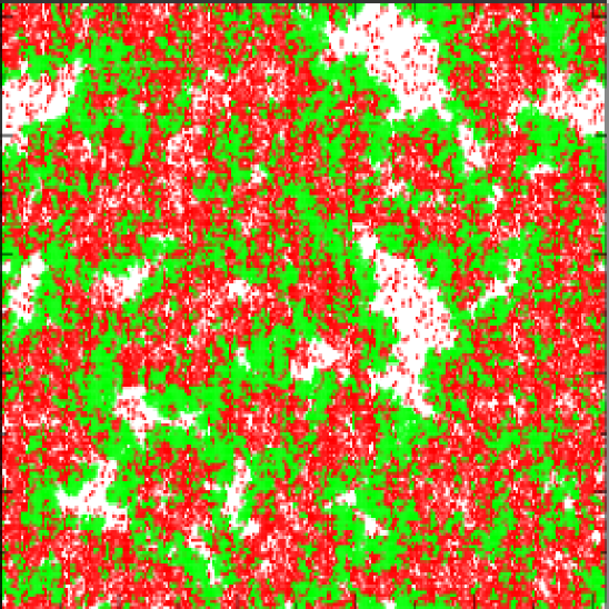
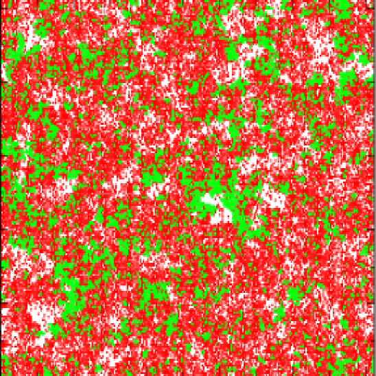
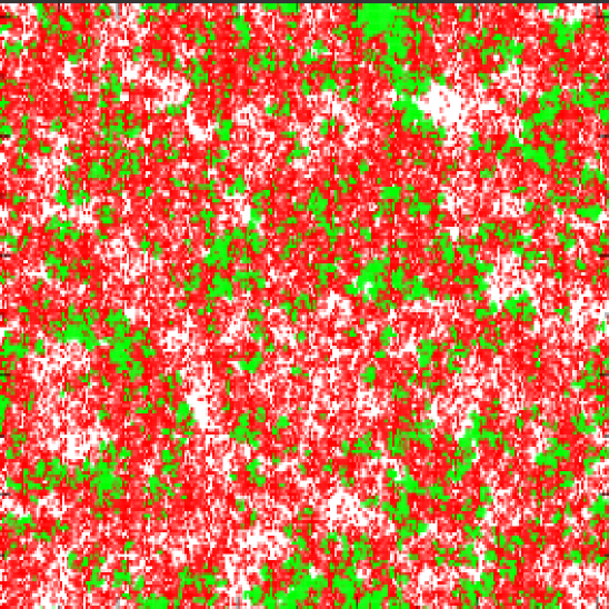
Figure 1: Snapshots of the spatial particle distribution for a single Monte Carlo simulation run of a stochastic Lotka–Volterra model on a $256\times 256$ square lattice with periodic boundary conditions, successively from left to right at $t=500$ Monte Carlo steps (MCS), $t=1000$ MCS, and $t=2000$ MCS, with reaction probabilities (see text) $\mu=0.025$, $\lambda=0.25$, and $\sigma=1.0$; only at most one particle per lattice site is allowed: sites occupied by predators are indicated in red, prey in green, while empty sites are shown white.

To model finite population carrying capacities caused by limited resources, one may restrict the local particle density or lattice site occupation number [14, 15, 20, 21, 22]. For the Lotka–Volterra model, this in turn introduces a new absorbing state, where the predator population goes extinct, while the prey proliferate through the entire system. By tuning the reaction rates as control parameters, one thus encounters a continuous active-to-absorbing state non-equilibrium phase transition [9, 10, 15, 16, 17, 20, 21]. In addition, near the predator extinction threshold, population oscillations cease, and both predator and prey concentrations directly relax exponentially to their quasi-stationary values [21]; c.f. Fig. 2.

Note that the existence of an absorbing state for the predator population, which cannot ever recover from extinction under the system’s stochastic dynamics, explicitly breaks the detailed balance conditions required for systems to effectively reside in a thermal equilibrium state. Generically, one expects continuous active-to-absorbing state transitions to be governed by the universal scaling properties of the directed percolation universality class (see, e.g., the overviews in Refs. [25, 26, 27]). This is in accord with the numerical data obtained in lattice Lotka–Volterra models; moreover, via representing the corresponding stochastic master equation through an equivalent Doi-Peliti pseudo-Hamiltonian and associated coherent-state functional integral, one can explicitly map the Lotka–Volterra model near the predator extinction threshold to Reggeon field theory that describes the directed percolation universality class [21, 24].

Induced by severe environmental changes in nature, certain ecosystems may collapse and at least some of its species face the danger of extinction. In order to monitor viability of populations and maintain ecological diversity, it is of great importance to identify appropriate statistical indicators that signify impending population collapse and may thus serve as early warning signals. In our simulations, we simply perform sudden predation rate switches to mimic fast environmental changes. If such a rate quench leads near the predator species extinction threshold, we observe the characteristic critical slowing-down and aging features expected at continuous phase transitions [25, 26, 27]. We demonstrate how either of these two characteristic dynamical signatures, but specifically the emergence of aging scaling, might be utilized as advanced warning signals for species extinction [28].

In the following Sec. 2, we describe our stochastic lattice Lotka–Volterra model with restricted site occupations and the Monte Carlo simulation algorithm. We then demonstrate in Sec. 3.1 that sudden rate changes within the two-species coexistence phase lead to exponentially fast relaxation. In contrast, Sec. 3.2 explores quenches to the critical predator extinction threshold, the ensuing critical slowing-down and algebraic predator density decay, as well as the critical aging scaling that we observe for the predator density autocorrelation function. Finally, Sec. 4 provides our conclusions.

2 Model Description and Simulation Protocol

We study a spatially extended stochastic Lotka-Volterra model by means of Monte Carlo simulations performed on a two-dimensional square lattice with $1024\times 1024$ sites, subject to periodic boundary conditions; we largely follow the procedures described in Refs. [20, 21, 22]. In this work, we impose locally limited carrying capacities for each species through implementing lattice site occupation restrictions: The number of particles per lattice site can only be either $0$ or $1$; i.e., each lattice site can either be empty, occupied by a ‘predator’ $A$, or occupied by a ‘prey’ $B$ particle. The individual particles in the system undergo the following stochastic reaction processes:

$$A\binrel@{\rightarrow}\binrel@@{\mathop{\kern 0.0pt\rightarrow}\limits^{\widetilde{\mu}}}\emptyset\,,\quad A+B\binrel@{\rightarrow}\binrel@@{\mathop{\kern 0.0pt\rightarrow}\limits^{\widetilde{\lambda}}}A+A\,,\quad B\binrel@{\rightarrow}\binrel@@{\mathop{\kern 0.0pt\rightarrow}\limits^{\widetilde{\sigma}}}B+B\,.$$ (1)

The predators $A$ thus spontaneously die with decay rate $\widetilde{\mu}>0$. Upon encounter, they may also consume a prey particle $B$ located on a lattice site adjacent to theirs, and simultaneously reproduce with ‘predation’ rate $\widetilde{\lambda}>0$. Hence the $B$ particle on the nearest-neighbor site to the predator becomes replaced by another $A$ particle. We remark that in a more realistic description, predation and predator offspring production should naturally be treated as separate stochastic processes. While such an explicit separation induces very different dynamical behavior on a mean-field rate equation level, it turns out that in dimensions $d<4$ the corresponding stochastic spatially extended system displays qualitatively the very same features as the simplified reaction scheme (1) [20].

Prey in turn may reproduce with birth rate $\widetilde{\sigma}>0$, with the offspring particles placed on one of their parent’s nearest-neighbor sites. Note that we do not include nearest-neighbor hopping processes here. Instead, diffusive particle spreading is effectively generated through the reproduction processes that involve placement of the offspring onto adjacent lattice sites; earlier work has ascertained that incorporating hopping processes (with rate $\widetilde{D}$) independent of particle production yields no qualitative changes [21], except for extremely fast diffusion $\widetilde{D}\gg\widetilde{\mu},\widetilde{\lambda},\widetilde{\sigma}$, which leads to effective homogenization and consequent suppression of spatial correlations. One Monte Carlo Step (MCS) is considered completed when on average all particles have participated in the above reactions once. In our present study, we will hold the rates $\widetilde{\mu}$ and $\widetilde{\sigma}$ fixed while varying $\widetilde{\lambda}$ as our control parameter.

In general, the detailed Monte Carlo algorithm for the stochastic lattice Lotka–Volterra model proceeds as follows [21]:

• Select a lattice occupant at random and generate a random number $r$ uniformly distributed in the range $[0,1]$ to perform either of the following four possible reactions (with probabilities $D$, $\mu$, $\lambda$, and $\sigma$ in the range $[0,1]$):

• If $r<1/4$, select one of the four sites adjacent to this occupant, and move the occupant there with probability $D$, provided the selected neighboring site is empty (nearest-neighbor hopping).

• If $1/4\leq r<1/2$ and if the occupant is an $A$ particle, then with probability $\mu$ the site will become empty (predator death, $A\rightarrow\emptyset$).

• If $1/2\leq r<3/4$ and if the occupant is an $A$ particle, choose a neighboring site at random; if that selected neighboring site holds a $B$ particle, then with probability $\lambda$ it becomes replaced with an $A$ particle (predation reaction, $A+B\rightarrow A+A$).

• If $3/4\leq r<1$ and if the occupant is a $B$ particle, randomly select a neighboring site; if that site is empty, then with probability $\sigma$ a new $B$ particle is placed on this neighboring site (prey offspring production, $B\rightarrow B+B$).

To clarify our algorithm, we discuss a simple example: If $r$ is generated to be $0.1$, the first case applies, whence we need to perform nearest-neighbor hopping with probability $D$. Since for simplicity we set $D=0$ in our simulation, we just skip this step and proceed to generate a new random number $r$. We remark that different versions of similar simulation algorithms can naturally be implemented wherein the microscopic reaction processes and their ordering are varied. However, macroscopic long-time simulation results should not qualitatively differ for such variations, only the effective reaction rates $\widetilde{\mu}$, $\widetilde{\lambda}$, $\widetilde{\sigma}$ in (1), and the diffusivity $\widetilde{D}$ that result from the microscopic probabilities $\mu$, $\lambda$, $\sigma$, and $D$, and the overall time scale will need to be rescaled accordingly.

Figures 1 and 2 show the results of typical Monte Carlo simulation runs in two-dimensional stochastic lattice Lotka–Volterra models with periodic boundary conditions and site occupations restricted to at most a single predator ($A$) or prey ($B$) particle; thus both their local and mean densities are restricted to the range $\rho_{A}+\rho_{B}\leq 1$. Here, $\rho_{A/B}(t)$ is defined as the total predator (prey) number at time $t$ divided by the number of lattice sites $(1024)^{2}$. The snapshots at various simulation times in Fig. 1 visualize the early spreading activity fronts in the two-species coexistence phase, i.e., prey (green) invading empty (white) regions followed by predators (red), which induce the initial large-amplitude population oscillations. At longer run times, the prey here localize into fluctuating clusters, and the net population densities reach their quasi-stationary values. In the prey vs. predator density phase plot depicted in Fig. 2, the associated trajectory (iii) is a spiral converging to the asymptotic density values. Upon approaching the predator extinction threshold (holding $\mu$ and $\sigma$ fixed, at lower values of $\lambda)$, the population oscillations cease and the trajectory (ii) relaxes directly to the quasi-stationary coexistence state. Finally, below the extinction threshold (i), the predator population dies out, and the prey particles eventually fill the entire lattice.

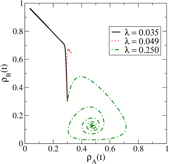
Figure 2: Monte Carlo simulation trajectories for a stochastic Lotka–Volterra model on a $1024\times 1024$ square lattice with periodic boundary conditions and restricted site occupancy (at most one particle allowed on each lattice site) shown in the predator $\rho_{A}(t)$ versus prey density $\rho_{B}(t)$ phase plane ($\rho_{A}+\rho_{B}\leq 1$) with initial values $\rho_{A}(0)=0.3=\rho_{B}(0)$, fixed reaction probabilities $\mu=0.025$, $\sigma=1.0$, and different predation efficiencies: (i) $\lambda=0.035$ (solid black): predator extinction phase; (ii) $\lambda=0.049$ (red dashed): direct exponential relaxation to the quasi-stationary state just above the extinction threshold in the predator-prey coexistence phase; (iii) $\lambda=0.250$ (green dash-dotted): the trajectories spiral into a stable fixed point, signifying damped oscillations deep in the coexistence phase.

3 Results

3.1 Relaxation dynamics within the coexistence phase

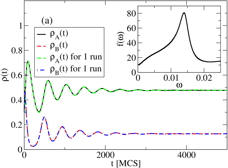
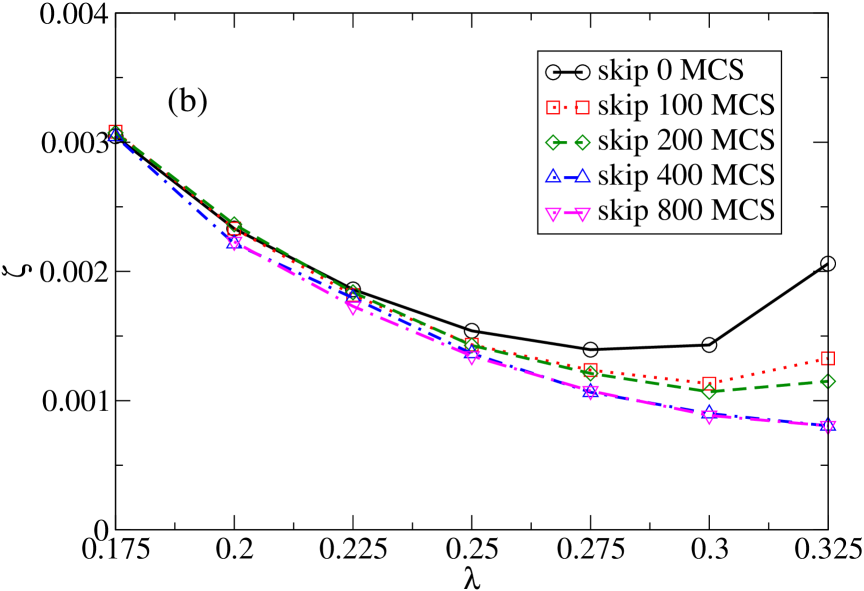
Figure 3: Monte Carlo simulation data for a stochastic Lotka–Volterra model on a $1024\times 1024$ square lattice with periodic boundary conditions: (a) Temporal evolution of the mean predator density $\rho_{A}(t)$ and the mean prey density $\rho_{B}(t)$ for fixed reaction probabilities $\mu=0.025$, $\lambda=0.25$, and $\sigma=1.0$, with initial densities $\rho_{A}(0)=0.3=\rho_{B}(0)$ (single runs shown in green / blue; the black and red curves are from data averaged over $200$ independent simulation runs). The inset shows the absolute value of the Fourier transform $f_{A}(\omega)$ of $\rho_{A}(t)$ (black curve). (b) Measured damping rate $\zeta$ in MCS^-1, as obtained from the peak half-width of $f_{A}(\omega)$, as function of the predation rate $\lambda$, when respectively $\Delta t=0$, $100$, $200$, $400$, and $800$ (top to bottom) initial MCS are skipped in the time series $\rho_{A}(t)$ as the Fourier transform is performed.

To set the stage, we first consider the time evolution of our stochastic Lotka–Volterra system on a two-dimensional lattice starting from a random initial configuration with the rate parameters set such that the model resides within the active coexistence state: the mean densities for both predator and prey species will thus remain positive and asymptotically reach constant values. Figure 3(a) shows the time evolution of the mean population densities $\rho_{A}(t)$ and $\rho_{B}(t)$, averaged over the entire lattice, both for single Monte Carlo simulations as well as data that result from averaging over $200$ independent runs. As is apparent in Fig. 1, already in moderately large lattices there emerge almost independent spatially separated population patches. The system is thus effectively self-averaging; as a consequence, the mean data from multiple runs essentially coincide with those from single ones. The reaction rates in the scheme (1) constitute the only control parameters in our system. Thus, if we fix the probabilities $\sigma$ and $\mu$, the predation probability $\lambda$ fully determines the final state. For generating the data in Fig. 3, we used constant reaction probabilities $\mu=0.025$, $\lambda=0.25$, and $\sigma=1.0$. The particles of both species are initially distributed randomly on the lattice with equal densities $\rho_{A}(0)=0.3=\rho_{B}(0)$.

In the early-time regime, the population densities are non-stationary and oscillate with an exponentially decreasing amplitude $\sim e^{-\zeta t}=e^{-t/t_{c}}$. We may utilize the damping rate $\zeta$ or decay time $t_{c}=1/\zeta$ to quantitatively describe the relaxation process towards the quasi-steady state. Since $\zeta$ is identical for both species, we just obtain this relaxation rate from the predator density decay via measuring the half-peak width of the absolute value of the Fourier transform of the time signal, $f_{A}(\omega)=\left|\int\rho_{A}(t)\,e^{i\omega t}\,dt\right|$. Alternatively, one might employ a direct fit in the time domain to damped oscillations. However, such a procedure is usually less accurate, as the early-time regime tends to be assigned too much weight in determining the fit parameters. Using the temporal Fourier transform and deducing the damping rate from the peak width in frequency space constitutes a numerically superior method. For example, for the predator density $\rho_{A}(t)$ shown in Fig. 3(a), the Fourier transform displayed in the inset yields $t_{c}\approx 650$ MCS. Indeed, by $t=3000$ MCS $\approx 5\,t_{c}$, the system has clearly reached its quasi-stationary state.

In the following, we aim to ascertain that the stochastic lattice Lotka–Volterra model loses any memory of its initial configuration once it has evolved for a duration $t>t_{c}$. We set the initial configuration at $t=0$ to be a random spatial distribution of particles with densities $\rho_{A}(0)=0.3=\rho_{B}(0)$, and hold $\mu=0.025$ and $\sigma=1.0$ fixed. We then record the relaxation kinetics for various values of $\lambda$, all in the interval $[0.175,0.325]$ to ensure that the final states reside deep within the species coexistence region, and measure the associated damping rates $\zeta$. The full black line in Fig. 3(b) plots the resulting function $\zeta(\lambda)$; the relaxation rate is indeed predominantly determined just by the reaction rates, but also influenced by the system’s initial state. The initial configuration effects can however be removed in a straightforward manner as follows: In the evaluation of the Fourier transform $f_{A}(\omega)$, we skip a certain initial MCS interval $\Delta t$ and just use the remaining data for $\rho_{A}(t)$ rather than the entire time sequence. If in fact the initial configuration only affects the system up to time $t\approx t_{c}$, the thereby obtained values of the function $\zeta(\lambda)$ should become independent of the length of the discarded initial time interval $\Delta t$ once $\Delta t>t_{c}(\lambda)$.

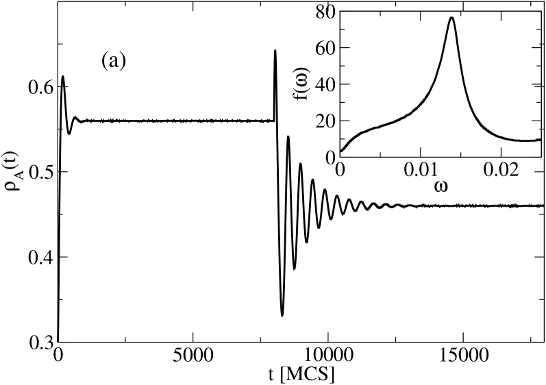
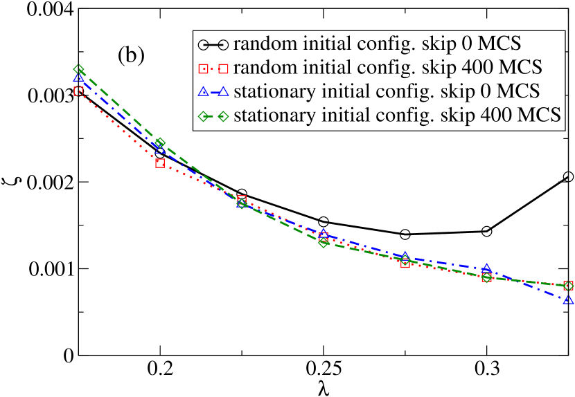
Figure 4: Monte Carlo simulation data for the predation rate quench scenario within the predator-prey coexistence phase on a $1024\times 1024$ square lattice with periodic boundary conditions (data averaged over $200$ independent simulation runs): (a) The main plot shows the temporal evolution of the mean predator density $\rho_{A}(t)$ for $\mu=0.025$, $\sigma=1.0$, $\rho_{A/B}(0)=0.3$. At $t_{1}=8000$ MCS, the predation probability is suddenly switched from $\lambda_{1}=0.125$ to $\lambda_{2}=0.275$. The inset displays the absolute value of the Fourier transform $f_{A}(\omega)$ of the time series after the quench ($t>t_{1}$). (b) Measured damping rate $\zeta(\lambda)$ when the system starts from a random initial condition with skipped initial time interval duration $\Delta t=0$ (full black line) or $400$ MCS (red dotted line; same data as in Fig. 3(b)), and following a quench from a quasi-steady state, where $\Delta t=0$ (blue dash-dotted) and $\Delta t=400$ MCS (green dashed).

In Fig. 3(b), we display the functions $\zeta(\lambda)$ obtained for various skipped initial time interval lengths $\Delta t$, ranging from $0$ to $800$ MCS. For large values of the predation probability $\lambda$, and ensuing long relaxation times $t_{c}(\lambda)=1/\zeta(\lambda)$, a marked dependence on $\Delta t$ is apparent. Yet for the entire $\lambda$ range under investigation, the two curves for $\Delta t=400$ MCS and $800$ MCS overlap (and we have checked this holds also for other values of $\Delta t>400$ MCS). Consequently, any dependencies on the initial configurations in the function $\zeta(\lambda)$ have been removed once $\Delta t>400$ MCS. This already gives a rough estimate for the typical relaxation rate, $\zeta\approx 0.0025$ MCS^-1, which indeed nicely matches the actual values seen in Fig. 3(b).

Next we check and confirm the above conclusions by considering a set of completely different initial configurations: Starting again from a random particle distribution with initial particle densities $\rho_{A}(0)=0.3=\rho_{B}(0)$, we first let the system relax to its quasi-steady state at prescribed reaction probabilities $\mu=0.025$, $\sigma=1.0$, and $\lambda_{1}=0.125$. Then we suddenly switch the predation probability to a new value $\lambda_{2}$. As a consequence, the system is driven away from the close to stationary, spatially highly correlated configurations that are characterized by well-formed domains of predators and prey, and relaxes towards a new stable quasi-steady state. Figure 4(a) illustrates such a ‘quench’ scenario: At $t_{1}=8000$ MCS, the predation probability is instantaneously changed from the initial value $\lambda_{1}=0.125$ to $\lambda_{2}=0.275$; it is apparent that the predation rate switch once again induces large transient population oscillations. We measure the ensuing relaxation rate $\zeta(\lambda)$ as function of the post-quench predation probability $\lambda=\lambda_{2}$ following the procedures outlined above, and with $\lambda_{2}$ in the interval $[0.175,0.325]$. In Fig. 4(b) we plot the result, if in the computation of the Fourier transform $f_{A}(\omega)$ an initial time interval of duration $\Delta t=400$ MCS is skipped (green dashed curve). For comparison, we also show the data for $\Delta t=0$ (blue dash-dotted) and replot the corresponding graphs for $\Delta t=0$ (black line) and $\Delta t=400$ MCS (red dotted) obtained for spatially random initial configurations. Both functions $\zeta(\lambda)$ with $\Delta t=400$ MCS overlap with the one for $\Delta t=0$ initiated in the quasi-steady state: Once $\Delta t>t_{c}(\lambda)$, the system’s initial states (here, spatially random or correlated) have no noticeable influence on the functional dependence of the relaxation rate on $\lambda$.

3.2 Relaxation kinetics following critical quenches

In the stochastic lattice Lotka–Volterra model with limited local carrying capacity, there exists an active-to-absorbing phase transition, namely an extinction threshold for the predator population, as illustrated in Fig. 2 and Fig. 5. Here, our Monte Carlo simulation runs were initiated with randomly placed predator and prey particles with densities $\rho_{A}(0)=0.3=\rho_{B}(0)$ and reaction probabilities $\mu=0.025$, $\sigma=1.0$, and $\lambda_{1}=0.250$. After $t_{1}=8000$ MCS, when the system has clearly reached its quasi-steady state, we suddenly switch the predation probability from $\lambda_{1}$ to much lower values $\lambda_{2}$ in the range $[0.03,0.05]$, which reside in the vicinity of the extinction critical point. The curves in Fig. 5 show the ensuing time evolution for the mean predator density $\rho_{A}(t)$. For small $\lambda_{2}$, all predator particles disappear, and eventually only the prey species survives, in contrast to the active two-species coexistence phase at larger $\lambda_{2}$ values, where both species persist with finite, stable mean population densities. In this subsection, we investigate in detail the non-equilibrium relaxation properties and ensuing dynamic scaling behavior following the quench from a quasi-steady coexistence state to the critical point.

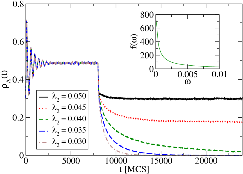
Figure 5: Monte Carlo simulation data (single runs) for the mean predator density $\rho_{A}(t)$ with $\rho_{A/B}(0)=0.3$ on a $1024\times 1024$ square lattice with periodic boundary conditions: The initial reaction probabilities are set to $\mu=0.025$, $\sigma=1.0$, and $\lambda_{1}=0.250$; at $t_{1}=8000$ MCS the system is quenched into the vicinity of the critical predator extinction point via switching the predation probability to $\lambda_{2}=0.050$, $0.045$, $0.040$, $0.035$, and $0.030$ (top to bottom). The inset shows the absolute value $f_{A}(\omega)$ of the Fourier transform of $\rho_{A}(t)$ for $\lambda_{2}=0.040$ after the quench.

$d=2$	SLLVM	DP sim.	DP exp.
$\alpha$	0.540(7)	0.4505(10) [29]	0.48(5) [31]
$z\,\nu$	1.208(167)	1.2950(60) [30]	1.29(11) [31]
$\Lambda_{c}/z$	2.37(19)	2.8(3) [32]	2.5(1) [31]
$b$	0.879(5)	0.901(2) [32]	0.9(1) [31]

Table 1: Monte Carlo simulation results for the critical exponents near the predator extinction threshold in the stochastic lattice Lotka–Volterra model (SLLVM) on a square lattice. For comparison, the table also lists the accepted literature scaling exponents for the directed percolation (DP) universality class [29, 30] as well as experimental values measured in turbulent liquid crystals (MBBA) [31]. The critical aging scaling exponents as obtained in our simulations along with earlier numerical results for the contact process [32] and experimental data [31] are included as well. The numbers in brackets indicate the estimated uncertainty in the last digits.

Near the active-to-absorbing phase transition, in our two-dimensional stochastic Lotka–Volterra model located at $\lambda_{c}=0.0416\pm 0.0001$ for fixed $\mu=0.025$ and $\sigma=1.0$, one should anticipate the standard critical dynamics phenomenology for continuous phase transitions [25, 27]: Fluctuations become prominent, and increasingly large spatial regions behave cooperatively, as indicated by a diverging correlation length $\xi(\tau)\sim|\tau|^{-\nu}$, where $\tau=(\lambda/\lambda_{c})-1$. Consequently, the characteristic relaxation time should scale as

$$t_{c}(\tau)\sim\xi(\tau)^{z}\sim|\tau|^{-z\,\nu}\ ,$$ (2)

implying a drastic critical slowing-down of the associated dynamical processes. Thus, exponential relaxation with time becomes replaced by much slower algebraic decay of the predator population density precisely at its extinction threshold $\lambda_{c}$,

$$\tau=0:\ \rho_{A}(t)\sim t^{-\alpha}\ .$$ (3)

The values of the three independent critical scaling exponents $\nu$, $z$, and $\alpha$ characterize certain dynamical universality classes. Generically, one expects active-to-absorbing phase transitions to be governed by the critical exponents of directed percolation (DP) [25, 27]; the middle column in Table 1 lists the established numerical literature values (from Refs. [29, 30]) for $\alpha$ and the product $z\,\nu$ in two dimensions. Indeed, standard field-theoretic procedures allow a mapping of the near-critical stochastic spatial Lotka–Volterra system to Reggeon field theory [21, 24], which represents the effective field theory for critical directed percolation [33, 27].

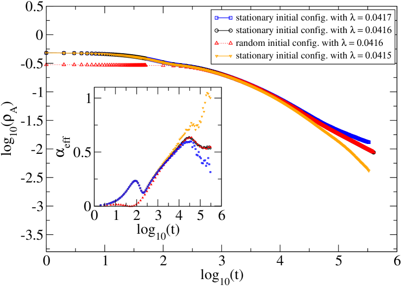
Figure 6: Double-logarithmic plot of the mean predator density decay $\rho_{A}(t)$ at the critical extinction threshold $\lambda_{c}=0.0416$ for fixed $\mu=0.025$ and $\sigma=1.0$, for both quasi-stationary (top, black) and random (lower curve, red dotted) initial configurations (data averaged over $2000$ independent simulation runs). For comparison, the predator density decay data are shown also for $\lambda=0.0417$ (blue, active coexistence phase) and $\lambda=0.0415$ (orange, absorbing predator extinction phase). The graphs in the inset show the local negative slopes of the curves in the main panel (using intervals of size $0.05$), i.e., the time-dependent effective critical decay exponent $\alpha_{\rm eff}(t)$.

In order to analyze the dynamic critical scaling behavior at the predator population extinction threshold, we follow the protocol outlined above and shown in Fig. 5, and first let the system relax to its quasi-steady state with a large predation probability $\lambda_{1}=0.250$. After $8000$ MCS, we quench the system to its critical point by switching this probability instantaneously to $\lambda_{c}=0.0416$. In order to acquire decent statistics, we perform $2000$ independent Monte Carlo simulation runs and then average our results. Figure 6 shows a double-logarithmic plot of the decay of the mean predator density $\rho_{A}(t)$ following the quench (top black curve); the inset displays the measured local slope of this graph (taken with intervals of size $0.05$), which can be interpreted as a time-dependent effective critical decay exponent $\alpha_{\rm eff}(t)=-d\log\rho_{A}(t)/d\log t$. A clean power law decay is thus reached when the slope stays constant, which in our data happens only quite late, at $t>10^{5}$ MCS. An asymptotically constant slope is observed as long as the value of $\lambda_{2}$ is sufficiently close to the critical point $\lambda_{c}$. Our simulation data (in the rather short time interval with constant $\alpha_{\rm eff}$) yield the critical decay exponent value $\alpha=0.54\pm 0.007$; we note that the accepted directed percolation universality class value is $\alpha\approx 0.4505$, which has been obtained by performing activity spreading simulations [29], see also Ref. [21]. For comparison, we also display the data for quenches to $\lambda=0.0417$ (blue curve) and $\lambda=0.0415$ (orange): In the former case, the predator density approaches a finite value as the system is still, albeit barely, in the active two-species coexistence phase, while for the lower predation rate the absorbing state is reached, with the predator population going extinct.

We wish to ascertain the independence of the asymptotic critical exponent $\alpha=\alpha_{\rm eff}(t\to\infty)$ from the starting configurations in our simulations. To this end, we directly initialize our stochastic lattice Lotka–Volterra system with reaction probabilities $\mu=0.025$, $\sigma=1.0$, and $\lambda=\lambda_{c}=0.0416$. The resulting Monte Carlo data, averaged over again $2000$ independent runs, are also shown in Fig. 6 (lower, dotted red curve). It is apparent that for the selected parameter values, the initial conditions become irrelevant for $t>1000$ MCS, whereafter our results for random and correlated quasi-steady state initial conditions perfectly overlap.

As visible in Fig. 5, the stochastic spatial Lotka–Volterra system immediately senses the predation rate change and the predator density decreases rapidly after the quench; for a very brief time period (about $200$ MCS), this decay is in fact independent of the new predation probability $\lambda_{2}$. Subsequently, the relaxation curves are quite sensitive to the selected value of $\lambda_{2}$. We measure the ensuing relaxation times $t_{c}(\lambda_{2})$ through evaluating the temporal Fourier transform, while skipping an initial time interval of duration $\Delta t=200$ MCS right after the quench in accord with the previous observation, averaging over $500$ independent Monte Carlo simulation runs. Figure 7 depicts our numerically determined relaxation time data for $t_{c}$ as a function of $\lambda_{2}$ in the vicinity of the critical predator extinction threshold $\lambda_{c}$. Note in the left inset that since we only consider a finite time interval (at most $128000$ MCS) after the quench for the computation of $f_{A}(\omega)$, our thus measured relaxation times do not diverge, but display a peak as function of $\lambda_{2}$ that becomes both more pronounced and sharper as the duration of the Monte Carlo simulation is increased. Indeed, we can estimate the critical value $\lambda_{c}$ from the peak position of the data curve for the longest simulations runs.

Since the left part of the graph turns out considerably smoother than the right part, we perform a power law fit only to the corresponding data subset ($\tau<0$). As shown in the main panel of Fig. 7, this yields the critical exponent product $z\,\nu=1.208\pm 0.167$; within our statistical error bars this is in reasonable agreement with the two-dimensional directed percolation literature values $\nu\approx 0.7333$ and $z=1.7660$ [25], i.e., $z\,\nu\approx 1.295$ [30]. The right inset displays the local time-dependent effective exponent $(z\,\nu)_{\rm eff}(t)=-d\log t_{c}(\tau)/d\log|\tau|$ for the longest simulation runs; the data appear not settled at a constant value yet, but indeed rather tend towards the slightly larger asymptotic DP value. Even with our longest Monte Carlo simulation runs, we have at best just barely reached the asymptotic scaling regime, and thus cannot very precisely determine the associated critical exponents for quasi-stationary observables.

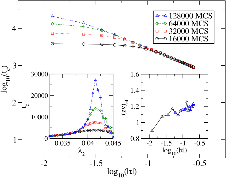
Figure 7: Characteristic relaxation time $t_{c}$ for the near-critical stochastic Lotka–Volterra model on a $1024\times 1024$ square lattice. The left inset shows the relaxation time $t_{c}(\lambda_{2})$ when the system is quenched from a quasi-stationary state at $\lambda_{1}=0.25$ to smaller values $\lambda_{2}$ in the vicinity of the predator extinction threshold $\lambda_{c}=0.0416$. The different curves indicate the resulting relaxation time estimates when respectively $128000$, $64000$, $32000$, and $16000$ MCS (top to bottom) were performed after the quench (all data averaged over $500$ independent simulation runs). The main panel displays the same data in double-logarithmic form. For $|\tau|=|(\lambda_{2}/\lambda_{c})-1|>0.1$, the different graphs overlap, collapsing onto a straight line with slope $-z\,\nu=-1.208\pm 0.167$. The right inset shows the associated local slope or effective exponent $(z\,\nu)_{\rm eff}(t)$ that appears to tend towards $z\,\nu\approx 1.3$.

A remarkable experiment with yeast cells has recently demonstrated a drastic increase in the relaxation time of the dynamics for a biological system near its population extinction threshold [28]. The authors therefore propose to utilize critical slowing-down as an indicator to provide advanced warning of an impending catastrophic population collapse. However, as we have demonstrated in our simulations, c.f. Figs. 6 and 7, the unique and universal power law features in the population density decay and divergence of the relaxation time are asymptotic phenomena and emerge only rather late, in our system after $t\approx 10^{5}$ MCS. Such a long required time period to unambiguously confirm an ecological system’s proximity to an irreversible tipping point may preclude timely interventions to save the endangered ecosystem. As we shall see in the following, the appearance of physical aging features in appropriate two-time observables may serve as more advantageous warning signals for population collapse, as they provide both earlier and often more accurate indications for critical behavior (see, e.g., Ref. [34]).

As a consequence of the drastic slowing-down of relaxation processes, near-critical systems hardly ever reach stationarity. During an extended transient period, time translation invariance is broken, and the initial configuration strongly influences the system: both these features characterize the phenomenon of physical aging [26]. In the vicinity of critical points as well as in a variety of other instances where algebraic growth and decay laws are prominent, the non-equilibrium aging kinetics is moreover governed by dynamical scaling laws. In our context, aging scaling is conveniently probed in the two-time particle density autocorrelation function

$$C(t,s)=\langle n_{i}(t)\,n_{i}(s)\rangle-\langle n_{i}(t)\rangle\,\langle n_{i}(s)\rangle\ ,$$ (4)

where $n_{i}(t)=0$ or $1$ indicates the occupation number (here, for the predators $A$) on lattice site $i$ at time $t$. The cumulant (4) thus measures local temporal correlations as function of the two time instants $s$ and $t>s$; we shall refer to $t$ and $s$ as the observation and waiting time, respectively.

In a stationary dynamical regime, reached for both $t,s>t_{c}$, time translation invariance should hold, implying that $C(t,s)$ becomes a function of the evolved time difference $t-s$ only. In the transient aging window, characterized by double time scale separation $t_{c}\gg t,s,t-s\gg t_{\rm mic}$, where $t_{\rm mic}$ represents typical microscopic time scales, one often encounters a simple aging scenario described by the dynamical scaling form

$$C(t,s)=s^{-b}\,f_{c}(t/s)\,,\quad f_{c}(y)\sim y^{-\Lambda_{c}/z}$$ (5)

with the aging scaling exponent $b$, and a scaling function $f_{c}$ that asymptotic obeys a power law decay in the long-time limit, governed by the ratio of the autocorrelation exponent $\Lambda_{c}$ and dynamic critical exponent $z$ [26]. Near continuous phase transitions both in and far from thermal equilibrium, the simple aging dynamical scaling form (5) can be derived by means of renormalization group methods [33, 27]. For directed percolation, the aging exponents are related to the quasi-stationary critical exponents through the scaling relations (in $d$ space dimensions) [26]

$$b=2\,\alpha\ ,\quad\Lambda_{c}/z=1+\alpha+d/z\ .$$ (6)

In perhaps the simplest lattice realization of the directed percolation universality class, the contact process, numerical simulations have confirmed the simple aging scaling form (5), with scaling exponents $b\approx 0.9$ and $\Lambda_{c}/z\approx 2.8$ in two dimensions, see Table 1 [32]. If universality holds near active-to-absorbing phase transitions, we should observe the same scaling properties at the predator extinction threshold in our stochastic lattice Lotka–Volterra model.

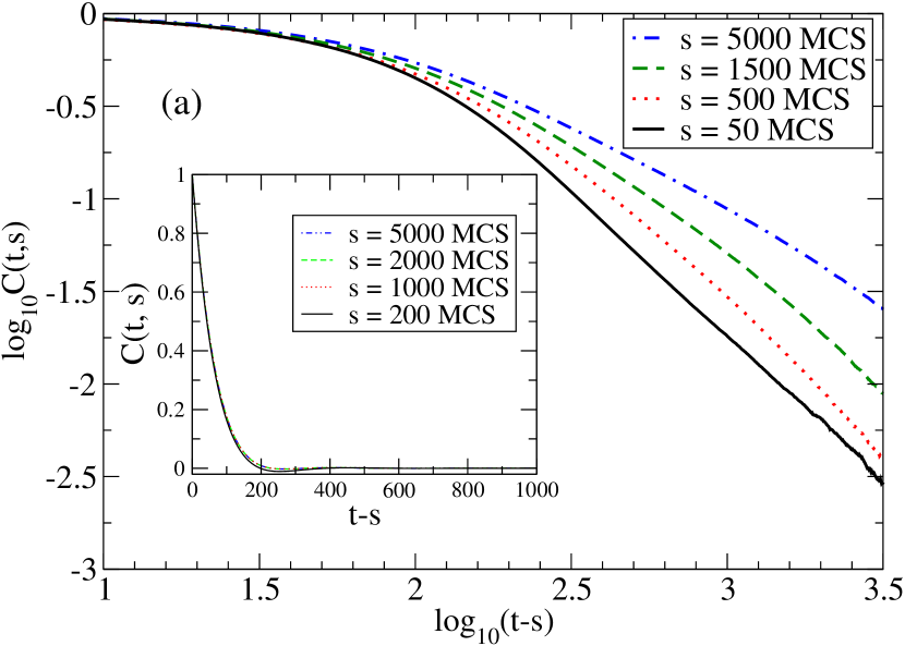
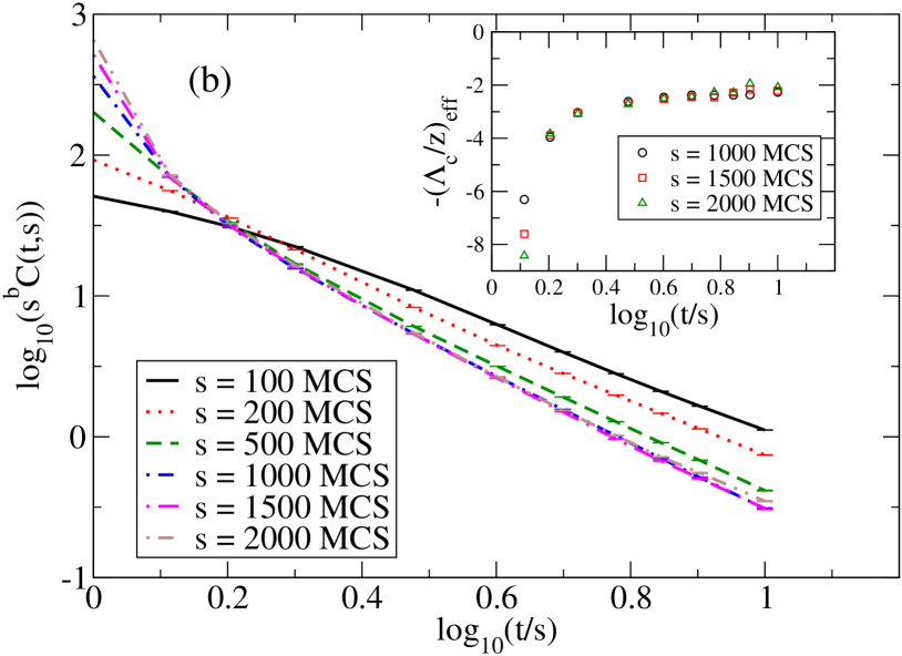
Figure 8: (a) Double-logarithmic plot of the predator density autocorrelation function $C(t,s)$ as a function of the time difference $t-s$ for various waiting times $s=50,500,1500,5000$ MCS (left to right) at the predator extinction critical point $\lambda_{c}=0.0416$; the data are averaged over $100$ independent simulation runs for each value of $s$. The inset shows that in contrast $C(t,s)$ decays exponentially fast for $\lambda_{2}=0.125$, i.e., a quench within the coexistence phase, and demonstrates that time translation invariance holds in this situation (data averaged over $400$ simulation runs for the waiting times $s=5000,2000,1000$, and $200$ (top to bottom). (b) Simple aging dynamical scaling analysis: $s^{b}\,C(t,s)$ is graphed versus the time ratio $t/s$, for $1000$ independent simulation runs for each waiting time $s$. The straight-slope section of the curves with large waiting times $s\geq 1000$ MCS yields $\Lambda_{c}/z=2.37\pm 0.19$, and the aging scaling exponent is determined to be $b=0.879\pm 0.005$. The inset displays the local effective exponent $-(\Lambda_{c}/z)_{\rm eff}(t)$.

In our Monte Carlo simulations, the predator density autocorrelation function $C(t,s)$ is obtained in a straightforward manner by monitoring the occupations of the lattice sites with $A$ particles following the previously discussed predation probability quench scenario to its critical value $\lambda_{c}$ after the system had first reached a quasi-stationary state. If time translation invariance applies, the ensuing curves of $C(t,s)$ plotted against $t-s$ should overlap for different values of the waiting time $s$. Indeed, this is clearly seen in the inset of Fig. 8(a) for the expected exponentially fast relaxation of the predator density autocorrelation function following a sudden quench from $\lambda_{1}=0.250$ to $\lambda_{2}=0.125$, whence the system remains within the two-species coexistence phase. In stark contrast, as becomes apparent in Fig. 8(a), time translation invariance is manifestly broken at the critical point.

In Fig. 8(b), we plot our data for the critical density autocorrelations, now averaged over $1000$ simulation runs, in the form of $s^{b}\,C(t,s)$ versus the time ratio $t/s$, for a set of waiting times $100$ MCS $\leq s\leq 2000$ MCS, in order to test for the simple aging dynamical scaling scenario (5). The aging exponent $b$ is determined by attempting to collapse the data for the three large waiting times $s\geq 1000$ MCS onto a single master curve. With the choice $b=0.879\pm 0.005$, the predator density autocorrelation function displays simple aging scaling for $s=1000$, $1500$, and $2000$ MCS. However, for small $s\leq 500$ MCS, the curves cannot be properly rescaled and collapsed. Depending on how many data points in the $t/s$ plot are used, one obtains slightly different values for $b$; their standard deviation gives our estimated errors. Within these error bars, the directed percolation scaling relation $b=2\,\alpha$ is just marginally fulfilled. We also remark that since our estimate for the location of the critical point $\lambda_{c}$ is inevitably measured only with limited accuracy, and we cannot meaningfully extend our finite-system simulation runs for arbitrarily long time periods, we also do not observe aging scaling anymore for $s\gg 2000$ MCS; to extend the aging analysis to larger waiting times would require both a more accurate measurement of $\lambda_{c}$ and larger simulation domains.

Finally, the exponent ratio $\Lambda_{c}/z$ may be estimated from the slope of the master curve in Fig. 8(b) resulting from the data collapse at large waiting times; see also the inset that shows the associated effective exponent. We find $\Lambda_{c}/z=2.37\pm 0.19$, which within the estimated error bars is in fair agreement with the value $2.8$ measured for the contact process in $d=2$ dimensions [32], and in accord with the scaling relation (6). To ascertain that the critical aging exponents do not depend on the initial configurations, we have repeated the above procedures for Monte Carlo simulations initiated with randomly distributed particles at the critical predation probability $\lambda_{c}$ rather than starting with the spatially correlated initial configurations prepared in quasi-steady states. We have confirmed that we thereby obtain identical values for $b$ and $\Lambda_{c}/z$, as listed in the first column of Table 1. Within our error bars these are in accord with the two-dimensional values obtained for the contact process [32] and in experiments on turbulent liquid crystals [31].

Figure 8(b) demonstrates that convincing critical aging scaling collapse is achieved for $t/s\geq 5$, or $t\approx 10^{4}$ MCS even for the longest waiting time $s=2000$ MCS under consideration here. Note that aging scaling thus appears by about a factor of $10$ earlier in the system’s temporal evolution than the critical power laws describing the quasi-stationary predator density decay and the divergence of the characteristic relaxation time. Just as critical slowing-down, the emergence of physical aging and certainly the associated dynamical scaling is an unambiguous indicator of the ecosystem’s proximity to population extinction. Critical aging scaling hence provides a complementary warning signal for impending collapse, yet becomes manifestly visible markedly earlier in the system’s time evolution.

We end our discussion of non-equilibrium relaxation processes in spatially extended stochastic Lotka–Volterra models by briefly addressing the sole remaining quench scenario, which takes the system from the active two-species coexistence state to the absorbing phase wherein the predator population goes extinct. Outside the critical parameter region, the characteristic relaxation time $t_{c}$ is finite; i.e., the mean predator density will decay to zero exponentially fast, as local predator clusters become increasingly dilute, while the prey gradually fill the entire system. In the absorbing state, population density fluctuations eventually cease, whence no interesting dynamical features remain.

4 Conclusion

To conclude, we have investigated non-equilibrium relaxation features in a stochastic Lotka–Volterra Model on a two-dimensional lattice via detailed Monte Carlo simulations. If the prey carrying capacity is limited, i.e., in the presence of site restrictions (and for sufficiently large system size), there appears a predator extinction threshold that separates an inactive phase wherein the prey proliferate and the predators die out, from an active phase where both species coexist and compete. In a first set of numerical experiments, we observe the system’s relaxation either from a random initial configuration or between two quasi-stationary states within the active coexistence phase via suddenly changing the predation rate. As expected, we find that the initial state generically only influences the subsequent oscillatory dynamics for the duration of about one characteristic relaxation time, implying that the system exponentially quickly loses any memory of the initial configuration.

Our main focus has thus been the analysis of critical quenches and the ensuing dynamical scaling behavior. Following a quench of the predation rate to its critical value for the predator species extinction threshold, we have measured the dynamic scaling exponents for the diverging relaxation time and the algebraic decay of the predator density. Within our systematic and statistical errors, we obtained the expected values for the directed percolation universality class that generically characterizes active-to-absorbing phase transitions. In addition, we have studied the critical aging properties of this system: Reflecting critical slowing-down, the characteristic relaxation time diverges at the extinction threshold; as a consequence, time translation invariance is broken, and physical aging governed by universal scaling features emerges. Our measured aging scaling exponents are close to those found previously for the contact process, which is perhaps the simplest lattice realization of the directed percolation universality class. We remark that at least to our knowledge, this present study constitutes only the second investigation of aging scaling at an active-to-absorbing phase transition, and hence provides a crucial test of universality for non-equilibrium critical phenomena.

We also emphasize that universal aging scaling sets in considerably earlier during the system’s time evolution than asymptotic quasi-stationary power laws emerge, and in addition often yields more accurate exponent estimates [34]. In comparison with detecting critical slowing-down, this critical aging effect might thus serve as a preferable and more reliable early warning signal for impending population collapse.

References

References

- [1] May R M 1973 Stability and complexity in model ecosystems vol 6 (Princeton: Princeton University Press)
- [2] Maynard Smith J 1974 Models in ecology (Cambridge: Cambridge University Press)
- [3] Hofbauer J and Sigmund K 1998 Evolutionary games and population dynamics (Cambridge: Cambridge University Press)
- [4] Murray J D 1989 Mathematical biology (New York: Springer-Verlag)
- [5] Neal D 2004 Introduction to population biology (Cambridge: Cambridge University Press)
- [6] Lotka A J 1920 Undamped oscillations derived from the law of mass action J. Am. Chem. Soc. 42 1595
- [7] Volterra V 1926 Fluctuations in the abundance of a species considered mathematically Nature 118 558
- [8] Matsuda H, Ogita N, Sasaki A and Satō K 1992 Statistical mechanics of population – the lattice Lotka–Volterra model Progr. Theor. Phys. 88 1035
- [9] Satulovsky J E and Tomé T 1994 Stochastic lattice gas model for a predator-prey system Phys. Rev. E 49 5073
- [10] Boccara N, Roblin O and Roger M 1994 Automata network predator-prey model with pursuit and evasion Phys. Rev. E 50 4531
- [11] Durrett R 1999 Stochastic spatial models SIAM Review 41 677
- [12] Provata A, Nicolis G and Baras F 1999 Oscillatory dynamics in low-dimensional supports: a lattice Lotka–-Volterra model J. Chem. Phys. 110 8361
- [13] Rozenfeld A F and Albano E V 1999 Study of a lattice-gas model for a prey–-predator system Physica A 266 322
- [14] Lipowski A 1999 Oscillatory behavior in a lattice prey-predator system Phys. Rev. E 60 5179
- [15] Lipowski A and Lipowska D 2000 Nonequilibrium phase transition in a lattice prey-predator system Physica A 276 456
- [16] Monetti R, Rozenfeld A and Albano E 2000 Study of interacting particle systems: the transition to the oscillatory behavior of a prey-predator model Physica A 283 52
- [17] Droz M and Pȩkalski A 2001 Coexistence in a predator-prey system Phys. Rev. E 63 051909
- [18] Antal T and Droz M 2001 Phase transitions and oscillations in a lattice prey-predator model Phys. Rev. E 63 056119
- [19] Kowalik M, Lipowski A and Ferreira A L 2002 Oscillations and dynamics in a two-dimensional prey-predator system Phys. Rev. E 66 066107
- [20] Mobilia M, Georgiev I T and Täuber U C 2006 Fluctuations and correlations in lattice models for predator-prey interaction Phys. Rev. E 73 040903
- [21] Mobilia M, Georgiev I T and Täuber U C 2007 Phase transitions and spatio-temporal fluctuations in stochastic lattice Lotka-–Volterra models J. Stat. Phys. 128 447
- [22] Washenberger M J, Mobilia M and Täuber U C 2007 Influence of local carrying capacity restrictions on stochastic predator–-prey models J. Phys. Cond. Matt. 19 065139
- [23] McKane A J and Newman T J 2005 Predator-prey cycles from resonant amplification of demographic stochasticity Phys. Rev. Lett. 94 218102
- [24] Täuber U C 2012 Population oscillations in spatial stochastic Lotka–-Volterra models: a field-theoretic perturbational analysis J. Phys. A: Math. Theor. 45 405002
- [25] Henkel M, Hinrichsen H and Lübeck S 2008 Non-equilibrium phase transitions vol 1: Absorbing phase transitions (Bristol, UK: Springer)
- [26] Henkel M and Pleimling M 2010 Non-equilibrium phase transitions vol 2: Ageing and dynamical scaling far from equilibrium (Bristol, UK: Springer)
- [27] Täuber U C 2014 Critical dynamics – A field theory approach to equilibrium and non-equilibrium scaling behavior (Cambridge: Cambridge University Press)
- [28] Dai L, Vorselen D, Korolev K S and Gore J 2012 Generic indicators for loss of resilience before a tipping point leading to population collapse Science 336 1175
- [29] Voigt C A and Ziff R M 1997 Epidemic analysis of the second-order transition in the Ziff-Gulari-Barshad surface-reaction model Phys. Rev. E 56 R6241
- [30] Grassberger P and Zhang Y-C 1996 Self-organized formulation of standard percolation phenomena Physica A 224 169
- [31] Takeuchi K A, Kuroda M, Chaté H and Sano M 2009 Experimental realization of directed percolation criticality in turbulent liquid crystals Phys. Rev. E 80 051116
- [32] Ramasco J J, Henkel M, Santos M A and da Silva Santos C A 2004 Ageing in the critical contact process: a Monte Carlo study J.Phys.A Math.Gen. 37 10497
- [33] Janssen H K and Täuber U C 2005 The field theory approach to percolation processes Ann. Phys. (NY) 315 147
- [34] Daquila GL and Täuber U C 2012 Nonequilibrium relaxation and critical aging for driven Ising lattice gases Phys. Rev. Lett. 108 110602