Monopole-Antimonopole Scattering

Abstract

We numerically study the head-on scattering of a ’t Hooft-Polyakov magnetic monopole and antimonopole for a wide range of parameters. In contrast to the scattering of a $\lambda\phi^{4}$ kink and antikink in 1+1 dimensions, we find that the monopole and antimonopole annihilate even when scattered at relativistic velocities. If the monopole and antimonopole have a relative twist, there is a repulsive force between them and they can initially be reflected. However, in every case we have examined, the reflected monopoles remain bound and eventually annihilate. We also calculate the magnetic helicity in the aftermath of monopole-antimonopole annihilation and confirm the conversion of relative twist to magnetic helicity as discussed earlier in the electroweak case.

Beautiful results have been obtained on the scattering of monopoles on monopoles Manton:1981mp ; AtiyahHitchinbook ; MantonSutcliffebook . For example, analytical techniques show that head-on collision leads to $90^{\circ}$ scattering for a certain value of the coupling constant (in the so-called Bogomolny-Prasad-Sommerfield (BPS) limit) AtiyahHitchinbook . Monopole-antimonopole scattering, though, has received less attention, perhaps because the process is less amenable to analysis.

A general expectation is that monopole-antimonopole (${\rm M\overline{M}}$ ) scattering will lead to their annihilation and the energy will be dissipated in the form of radiation. However this is not the result obtained in the analogous process of $Z_{2}$ kink-antikink scattering in 1+1 dimensions. Numerical studies of kink-antikink scattering show annihilation at low kinetic energy, reflection at higher incoming energy, followed by annihilation at yet higher energies, etc., yielding a band structure reminiscent of solutions of the Mathieu equation Campbell:1983xu ; Anninos:1991un . One motivation for the present work is to check for chaotic behavior in ${\rm M\overline{M}}$ scattering.

A second motivation for studying ${\rm M\overline{M}}$ scattering comes from the recent interest in the possible existence and detection of a helical inter-galactic magnetic field Tashiro:2013ita . Early work had speculated on the production of magnetic fields during monopole-antimonopole annihilation Vachaspati:1991nm ; Vachaspati:1994xc . The connection to baryogenesis was made when the electroweak sphaleron solution that mediates baryon number violation was interpreted in terms of electroweak ${\rm M\overline{M}}$ pairs Vachaspati:1994ng ; Hindmarsh:1993aw . It is crucial for this connection that monopole-antimonopole pairs can have a relative “twist” and the (unstable) electroweak sphaleron solution is really an ${\rm M\overline{M}}$ pair that is prevented from annihilating by the presence of a twist. In sphaleron decay, the twist is believed to be the reason that the resultant magnetic field has non-zero helicity, $h$, defined by

$$h=\int d^{3}x~{}{\bm{A}}\cdot{\bm{B}}$$ (1)

where ${\bm{A}}$ is the electromagnetic gauge potential and ${\bm{B}}$ is the magnetic field. In this paper, we will also study the scattering of twisted ${\rm M\overline{M}}$ pairs and confirm that magnetic field helicity originates in the relative twist of the ${\rm M\overline{M}}$ .

The results of our investigations are easily summarized: numerical evolution for a wide range of ${\rm M\overline{M}}$ initial conditions show that untwisted ${\rm M\overline{M}}$ scattering always leads to annihilation. Thus we do not see any evidence for chaotic behavior similar to that seen in 1+1 dimensions. However, when the monopoles are initially twisted, there is a repulsive force between the monopoles. At low velocities, the monopoles slow down or may even reflect back. Yet this reflection is temporary and soon reversed, and the ${\rm M\overline{M}}$ then annihilate. Further, the annihilation of twisted ${\rm M\overline{M}}$ results in the production of a helical magnetic field.

We start out in Sec. I by defining the field theory, describing the magnetic monopoles and the twisted ${\rm M\overline{M}}$ ansatz in which the monopoles are also Lorentz boosted. The ${\rm M\overline{M}}$ field ansatz will form the initial conditions for the numerical evolution described in Sec. II, where we also show sample plots of the scattering, the trajectories of the ${\rm M\overline{M}}$ , and the magnetic helicity generated during annihilation. We conclude in Sec. III.

I SO(3) Model, Monopoles, and ${\rm M\overline{M}}$ Ansatz

I.1 ${\rm SO(3)}$model

The model we study contains an ${\rm SO(3)}$adjoint scalar and gauge field, $\{\phi^{a},W_{\mu}^{a}\}$ ($a=1,2,3$) with the Lagrangian

$$L=\frac{1}{2}(D_{\mu}\phi)^{a}(D^{\mu}\phi)^{a}-\frac{1}{4}W^{a}_{\mu\nu}W^{a\mu\nu}-\frac{\lambda}{4}(\phi^{a}\phi^{a}-\eta^{2})^{2}$$ (2)

where,

$$(D_{\mu}\phi)^{a}=\partial_{\mu}\phi^{a}-igW^{c}_{\mu}(T^{c})^{ab}\phi^{b}$$ (3)

and the ${\rm SO(3)}$generators are $(T^{a})^{bc}=-i\epsilon^{abc}$. The gauge field strengths are defined by

$$W_{\mu\nu}^{a}=\partial_{\mu}W_{\nu}^{a}-\partial_{\nu}W_{\mu}^{a}+g\epsilon^{abc}W_{\mu}^{b}W_{\nu}^{c}.$$ (4)

The scalar field equations of motion are

$$\partial_{t}^{2}\phi^{a} = \partial_{i}\partial_{i}\phi^{a}+igW^{\mu c}(T^{c})^{ab}\partial_{\mu}\phi^{b}$$ (5)

$$+igW^{\mu c}(T^{c})^{ab}(D_{\mu}\phi)^{b}-\lambda(\phi^{b}\phi^{b}-\eta^{2})\phi^{a}.$$

We will work in the Lorenz gauge given by the equation

$$\partial_{t}W^{a}_{0}=\partial_{i}W^{a}_{i}$$ (6)

and then the gauge field equations are

$$\partial_{t}^{2}W^{a}_{\mu} = \partial_{i}\partial_{i}W^{a}_{\mu}-g\epsilon^{abc}W^{\nu b}\partial_{\nu}W_{\mu}^{c}-g\epsilon^{abc}W_{\nu}^{b}W^{\nu c}_{~{}\mu}$$ (7)

$$-g\epsilon^{abc}\phi^{b}(D_{\mu}\phi)^{c}.$$

By rescaling the coordinates and the fields, as we shall do from now on, we can set $g=1$ and $\eta=1$. Then $\lambda$ is the only free parameter left in the model. The BPS case is when $\lambda=0$. We will numerically evolve the 15 second order partial differential equations (PDE) in (5) and (7).

The energy density for the model is given by

$${\cal E} = \frac{1}{2}(D_{t}\phi)^{a}(D_{t}\phi)^{a}+\frac{1}{2}(D_{i}\phi)^{a}(D_{i}\phi)^{a}$$ (8)

$$+\frac{1}{2}(W^{a}_{0i}W^{a}_{0i}+W^{a}_{ij}W^{a}_{ij})+\frac{\lambda}{4}(\phi^{a}\phi^{a}-1)^{2}$$

where the sum over the repeated index $j$ is restricted to $j>i$.

Once $\phi^{a}$ acquires its vacuum expectation value, the model contains two massive gauge fields and one massless gauge field. The massless gauge field is

$$A_{\mu}=n^{a}W^{a}_{\mu}$$ (9)

where $n^{a}\equiv\phi^{a}/\sqrt{\phi^{b}\phi^{b}}$ is a unit vector at all spatial points. The field strength corresponding to the gauge field $A_{\mu}$ is defined as 'tHooft:1974qc

$$A_{\mu\nu} = n^{a}W^{a}_{\mu\nu}-\epsilon^{abc}n^{a}(D_{\mu}n)^{b}(D_{\nu}n)^{c}$$ (10)

$$= \partial_{\mu}A_{\nu}-\partial_{\nu}A_{\mu}-\epsilon^{abc}n^{a}\partial_{\mu}n^{b}\partial_{\nu}n^{c}.$$

This field strength definition correspond to the usual Maxwell electric and magnetic field only when the magnitude $|\phi|$ is constant. We shall apply them at late times after the monopoles have annihilated and when $|\phi|$ is approximately constant and non-zero everywhere.

I.2 Monopoles

The monopole solution takes the form

$$\phi^{a}=P(r){\hat{x}}^{a}$$ (11)

$$W^{a}_{i}=\frac{(1-K(r))}{r}\epsilon^{aij}{\hat{x}}^{j}$$ (12)

where ${\hat{x}}={\bm{x}}/r$ and $r$ is the (rescaled) spherical radial distance centered on the monopole. The profile functions $P(r)$, $K(r)$ are not known in closed form except in the BPS ($\lambda=0$) case Prasad:1975kr ; Bogomolny:1975de

$$P_{\rm BPS}(r)=\frac{1}{\tanh(r)}-\frac{1}{r},$$ (13)

$$K_{\rm BPS}(r)=\frac{r}{\sinh(r)}.$$ (14)

We will be studying the evolution of monopoles for a range of $\lambda$. A functional form that reduces to the BPS profile functions for $\lambda=0$ and has the correct asymptotic properties is

$$P(r)=\frac{1}{\tanh(r)}-(1+mr)\frac{e^{-mr}}{r}$$ (15)

$$K(r)=\frac{r}{\sinh(r)}$$ (16)

where $m=\sqrt{2\lambda}$ is the scalar particle mass (in $\eta=1$ units).

Next we will need to patch together a monopole and an antimonopole, with a relative twist, and also boost the monopole and antimonopole towards each other.

I.3 ${\rm M\overline{M}}$ Ansatz

A twisted monopole-antimonopole ansatz is known in the context of the electroweak model where the scalar field is an ${\rm SU(2)}$ doublet Vachaspati:1994ng . The form is

$$\Phi=\left(\begin{array}[]{c}\sin(\theta/2)\sin({\bar{\theta}}/2)e^{i\gamma}+\cos(\theta/2)\cos({\bar{\theta}}/2)\\ \sin(\theta/2)\cos({\bar{\theta}}/2)e^{i\varphi}-\cos(\theta/2)\sin({\bar{\theta}}/2)e^{i(\varphi-\gamma)}\end{array}\right)$$ (17)

where $\theta$ and ${\bar{\theta}}$ are the spherical angles centered on the monopole and antimonopole respectively (see Fig. 1), $\varphi$ is the azimuthal angle, and $\gamma$ is the twist. A little algebra shows that $\Phi^{\dagger}\Phi=1$.

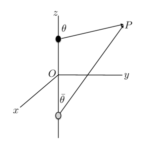
Figure 1: Monopole and antimonopole are chosen to be on the $z-$axis with some initial separation $2z_{0}$. The spherical angles $\theta$ and ${\bar{\theta}}$ are defined as shown.

From $\Phi$, we construct the corresponding unit vector field $n^{a}$ using

$$n^{a}=\Phi^{\dagger}\sigma^{a}\Phi$$ (18)

where $\sigma^{a}$ are the Pauli spin matrices. The result, with the replacement $\varphi\to\varphi-\gamma/2$ to make the expressions more symmetrical, is

$$n^{1} = (\sin\theta\cos{\bar{\theta}}\cos\gamma-\sin{\bar{\theta}}\cos\theta)\cos(\varphi-\gamma/2)$$ (19)

$$-\sin\theta\sin\gamma\sin(\varphi-\gamma/2)$$

$$n^{2} = (\sin\theta\cos{\bar{\theta}}\cos\gamma-\sin{\bar{\theta}}\cos\theta)\sin(\varphi-\gamma/2)$$ (20)

$$+\sin\theta\sin\gamma\cos(\varphi-\gamma/2)$$

$$n^{3} = \cos\theta\cos{\bar{\theta}}+\sin\theta\sin{\bar{\theta}}\cos\gamma$$ (21)

Close to the monopole, we have ${\bar{\theta}}\to 0$ and then

$$n^{1} \to \sin\theta\cos(\varphi+\gamma/2)$$ (22)

$$n^{2} \to \sin\theta\sin(\varphi+\gamma/2)$$ (23)

$$n^{3} \to \cos\theta$$ (24)

as we would expect around a monopole. Close to the antimonopole, we have $\theta\to\pi$ and then

$$n^{1} \to \sin{\bar{\theta}}\cos(\varphi-\gamma/2)$$ (25)

$$n^{2} \to \sin{\bar{\theta}}\sin(\varphi-\gamma/2)$$ (26)

$$n^{3} \to -\cos{\bar{\theta}}$$ (27)

which corresponds to an antimonopole (because of the minus sign in $n^{3}$). Also note the relative twist along $\varphi$ of the monopole and antimonopole.

Our ansatz has the nice feature that ${\hat{n}}\propto{\hat{z}}$ far away from the ${\rm M\overline{M}}$ in all directions when the twist vanishes. To check this we set $\gamma=0$, ${\bar{\theta}}\to\theta$ and obtain ${\hat{n}}=(0,0,1)$.

Now we are ready to write down the scalar field for a twisted monopole-antimonopole pair:

$$\phi^{a}(x,y,z)=P(r_{m})P(r_{\bar{m}})n^{a}$$ (28)

where $P(r)$ is the profile function in Eq. (15) and $r_{m}$, $r_{\bar{m}}$ are the distances of the spatial point $(x,y,z)$ from the monopole and antimonopole respectively.

At this stage the monopole-antimonopole are at rest. To boost the monopole along the $-z$ direction and the antimonopole along the $+z$ direction we first re-express $r_{m}$, $r_{\bar{m}}$ and $n^{a}$ in Cartesian coordinates

$$r_{m}=|{\bm{x}}-{\bm{x}}_{m}|,\ \ r_{\bar{m}}=|{\bm{x}}-{\bm{x}}_{\bar{m}}|$$ (29)

where ${\bm{x}}_{m}=(0,0,z_{0})$ and ${\bm{x}}_{\bar{m}}=(0,0,-z_{0})$ are the locations of the monopole and the antimonopole respectively. The unit vector $n^{a}$ is also expressed in Cartesian coordinates,

$$r_{m}r_{\bar{m}}n^{1} = (cx+sy)[(z+z_{0})\cos\gamma-(z-z_{0})]$$ (30)

$$-(cy-sx)r_{\bar{m}}\sin\gamma$$

$$r_{m}r_{\bar{m}}n^{2} = (cy-sx)[(z+z_{0})\cos\gamma-(z-z_{0})]$$ (31)

$$+(cx+sy)r_{\bar{m}}\sin\gamma$$

$$r_{m}r_{\bar{m}}n^{3} = (z-z_{0})(z+z_{0})+(x^{2}+y^{2})\cos\gamma$$ (32)

where $c\equiv\cos(\gamma/2)$, $s\equiv\sin(\gamma/2)$. Here we have been careful to distinguish the $(z\pm z_{0})$ factors coming from the monopole and antimonopole, since these will be boosted differently,

$$(z\pm z_{0})\to(z\pm z_{0})^{(b)}=\gamma_{L}((z\pm z_{0})\mp v_{z}t)$$ (33)

where, $\gamma_{L}=(1-v_{z}^{2})^{-1/2}$. Note that these boosts also have to be included in $r_{m}$ and $r_{\bar{m}}$. (We will denote boosted quantities by a $(b)$ superscript.) Then the scalar fields at $t=0$ for a boosted, twisted monopole-antimonopole pair are:

$$\phi^{a}(x,y,z)=\left[P(r_{m}^{(b)})P(r_{\bar{m}}^{(b)})n^{{(b)}a}\right]_{t=0}$$ (34)

We also need the first time derivative (denoted by an overdot) of the scalar field at $t=0$ and this is given by

$${\dot{\phi}}^{a}(x,y,z)=\left[\partial_{t}\left(P(r_{m}^{(b)})P(r_{\bar{m}}^{(b)})n^{{(b)}a}\right)\right]_{t=0}$$ (35)

The partial time derivative can be expressed in terms of spatial derivatives as discussed below.

Now that we have the initial scalar fields, we move on to specify the initial gauge fields. This is most simply done numerically using the following scheme. We fix the internal space orientation of the gauge fields by minimizing the covariant derivative. The vacuum solution of $D_{\mu}{\hat{n}}=0$ is

$$W^{a}_{\mu}|_{\rm vacuum}=-\epsilon^{abc}{\hat{n}}^{b}\partial_{\mu}{\hat{n}}^{c}$$ (36)

To this we attach profile functions so that the gauge fields are well defined at the locations of the monopole and antimonopole. So

$$\hskip-28.45274ptW^{a}_{\mu}|_{t=0} = -\biggl{[}(1-K(r_{m}^{(b)}))(1-K(r_{\bar{m}}^{(b)}))$$ (37)

$$\hskip 71.13188pt\times\epsilon^{abc}{\hat{n}}^{(b)b}\partial_{\mu}{\hat{n}}^{(b)c}\biggr{]}_{t=0}$$

Finally we need the initial time derivative of $W^{a}_{\mu}$. We shall treat the spatial and temporal components differently to enforce the Lorenz gauge condition. For the spatial components, as in the case of the scalar field, the time derivative is given by

$$\hskip-14.22636pt{\dot{W}}^{a}_{i}|_{t=0} = -\biggl{[}\partial_{t}\biggl{(}(1-K(r_{m}^{(b)}))(1-K(r_{\bar{m}}^{(b)}))$$ (38)

$$\hskip 71.13188pt\times\epsilon^{abc}{\hat{n}}^{(b)b}\partial_{i}{\hat{n}}^{(b)c}\biggr{)}\biggr{]}_{t=0}$$

For the time component of the gauge field, we use the Lorenz gauge condition

$${\dot{W}}^{a}_{0}|_{t=0}=[\partial_{i}W^{a}_{i}]_{t=0}$$ (39)

Although the form of the initial conditions is quite involved, they are not too difficult to implement since temporal derivatives can be related to spatial derivatives using

$$[(z\pm z_{0})^{(b)}]_{t=0}=\gamma_{L}(z\pm z_{0})$$ (40)

$$[\partial_{t}(z\pm z_{0})^{(b)}]_{t=0}=\mp\gamma_{L}v_{z}$$ (41)

and spatial derivatives can be evaluated numerically.

II Evolution

We discretize the $15\times 2$ first-order equations of motion and evolve the system using the iterated Crank-Nicholson method with two iterations Teukolsky:1999rm . Our code has the novelty that all field theory specific routines are generated symbolically and are then inserted into a PDE integrating routine. We have also implemented absorbing boundary conditions by assuming that all fields only depend on $t-r$ where $r$ is the distance from the center of the lattice. For the specific problem at hand, all the non-trivial dynamics is well within the simulation volume and the choice of boundary conditions is not crucial.

The initial energy of our ansatz for $\gamma=0$ matches the analytic result for untwisted BPS monopoles. During the numerical evolution we have checked energy conservation at the few percent level at early times, before energy can start leaving the simulation volume. The Lorenz gauge condition is also approximately satisfied at all times in the parameter space we have investigated.

The free parameters in the model are the coupling constant $\lambda$, the boost velocity $v_{z}$, and the twist $\gamma$. The initial separation is taken to be 0.3 times the semi-lattice size plus an offset that ensures that the magnitude of $\phi$ does not vanish on a lattice point at the initial time. (This simplifies some of the numerics.) We have also chosen $\lambda=1$ for our runs, and experimentation with a few other values (including $\lambda=0$) showed similar results. The initial boost velocity $v_{z}$ was varied in the interval $(0.1,0.9)$, and the twist angle was chosen to range from 0 to $2\pi$ in steps of $\pi/4$. The only runs where we do not explicitly see annihilation until the end of the simulation is in the case when $\gamma=\pi$ and for some low values of $v_{z}$. However, even in the cases when the ${\rm M\overline{M}}$ do not annihilate, they form a bound system and do not escape to infinity. In some cases, we have let the system evolve much longer and always found that the ${\rm M\overline{M}}$ eventually annihilate. In Fig. 2 we show snapshots of untwisted ${\rm M\overline{M}}$ and they simply come together and annihilate. In Fig. 3 we show snapshots of twisted ($\gamma=\pi$) ${\rm M\overline{M}}$ at the same times as for the untwisted case and we see that they have not yet annihilated.

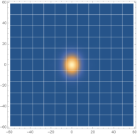
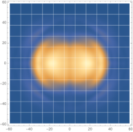
Figure 2: Snapshots of a planar slice of annihilating monopole and antimonopole for $\lambda=1$, $\gamma=0$, and $v_{z}=0.5$. The colors represent energy density.

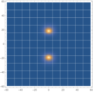
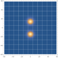
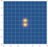
Figure 3: Snapshots of a planar slice of non-annihilating monopole and antimonopole for $\lambda=1$, $\gamma=\pi$, and $v_{z}=0.5$. Except for the twist, all parameters, including snapshot times, are identical to those in Fig. 2. The colors represent energy density. At yet later times, the monopoles back-scatter but are still bound and return to annihilate as discussed in the text.

We plot the location of the monopole as a function of time for a few sample parameters in Figs. 4 and 5. The monopole location is defined by the location of the minimum of $\phi^{a}\phi^{a}$ over the simulation volume for $z>0$ provided ${\rm min}[\sqrt{\phi^{a}\phi^{a}}]<0.25$. In Fig. 4, we hold the velocity fixed at 0.5 and vary the twist from 0 to $\pi$. (The dynamics for twist of $\gamma$ is the same as that for a twist of $2\pi-\gamma$.) It is clear from the plot that the twist slows down the monopole and can even cause it to bounce back. In Fig. 5 we show $z(t)$ for the monopole when the twist is held fixed at $\pi$ and $v_{z}=0.25,0.50,0.75$. Here the bounce back is very apparent. However, the monopoles are still bound after they bounce back and will eventually annihilate.

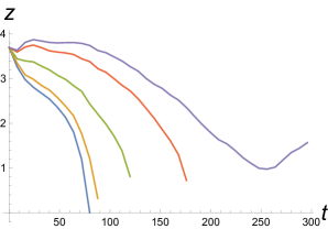
Figure 4: The z-coordinate of the monopole as a function of time for $\lambda=1$, $v_{z}=0.50$ and $\gamma/(\pi/4)=0,1,2,3,4$ (curves from left to right). The curves terminate once ${\rm min}[\sqrt{\phi^{a}\phi^{a}}]\geq 0.25$ (a condition that is met after the ${\rm M\overline{M}}$ have annihilated) except in the $\gamma=\pi$ case, when the ${\rm M\overline{M}}$ have not annihilated even by the end of the simulation run (300 time steps with $dt=dx/2=0.1$).

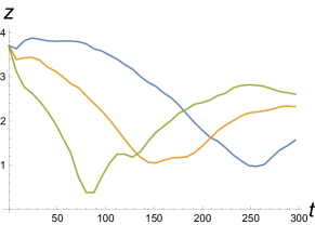
Figure 5: The z-coordinate of the monopole as a function of time for $\lambda=1$, $\gamma=\pi$, and $v_{z}=0.25,0.50,0.75$ (blue, orange and green curves). The ${\rm M\overline{M}}$ have not annihilated until the end of the simulation.

The untwisting and annihilation of the ${\rm M\overline{M}}$ is expected to radiate magnetic fields that are helical Copi:2008he ; Chu:2011tx . To test this expectation, we have calculated the helicity defined in Eq. (1) using (9) and (10). The plot of the magnetic helicity as a function of time is shown in Fig. 6 where we hold the velocity fixed at 0.75 and vary the twist. The plot shows that the helicity vanishes if there is no twist ($\gamma=0$). Also, we see that the $h(\gamma)=-h(2\pi-\gamma)$, and the helicity vanishes in the case $\gamma=\pi$ (though in this case the ${\rm M\overline{M}}$ survive until the end of the simulation). These observations can be understood if the helicity is due to the untwisting motion of the ${\rm M\overline{M}}$ . If $\gamma<\pi$, the ${\rm M\overline{M}}$ untwist in one direction and then annihilate, while if $\gamma>\pi$, the ${\rm M\overline{M}}$ untwist in the other direction so that $\gamma\to 2\pi$. The opposite senses of untwisting lead to the production of magnetic fields with opposite helicity. The value $\gamma=\pi$ is an unstable point where the ${\rm M\overline{M}}$ are unable to decide which way to untwist. Eventually numerical instabilities will cause untwisting in one way or the other. In Fig. 6 we also observe oscillations in the magnetic helicity, suggesting that there may be oscillations in the twist.

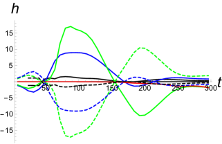
Figure 6: Magnetic helicity in the aftermath of ${\rm M\overline{M}}$ annihilation as a function of time for $\lambda=1$, $v_{z}=0.75$ and $\gamma/(\pi/4)=0,1,2,3,4,5,6,7$. The curves for $\gamma/(\pi/4)=0,4$ essentially coincide with $h=0$ and are not visible. The dashed curves are for $\gamma/(\pi/4)=5,6,7$ (green, blue, black), and mirror the solid curves for $\gamma/(\pi/4)=3,2,1$ (green, blue, black). This shows that $h(\gamma)=-h(2\pi-\gamma)$.

In Fig. 7 we plot the magnetic helicity for $\lambda=1$, $\gamma=3\pi/4$ and for $v_{z}=0.25,0.50,0.75$. The plots are similar in shape but shifted to earlier times for higher velocities. This can be understood because the ${\rm M\overline{M}}$ scatter at earlier times for higher velocities.

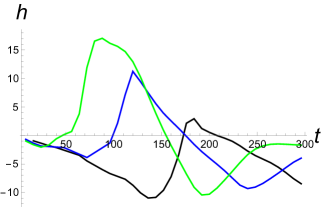
Figure 7: Magnetic helicity in the aftermath of ${\rm M\overline{M}}$ annihilation as a function of time for $\lambda=1$, $\gamma=3\pi/4$, and $v_{z}=0.25,0.50,0.75$ (black, blue and green curves).

III Conclusions

We have studied ${\rm M\overline{M}}$ scattering by numerical methods. Part of the challenge was to devise initial conditions that are suitable to describe boosted and twisted ${\rm M\overline{M}}$ . Our ansatz for initial conditions are given in Sec. I.3 but there may be other choices.

The numerical evolution of ${\rm M\overline{M}}$ shows that, unlike the scattering of kinks in 1+1 dimensions, ${\rm M\overline{M}}$ scattering is not chaotic, as the ${\rm M\overline{M}}$ are always found to annihilate over the wide range of parameters we have investigated. A twist in the initial conditions produces a repulsive force between the monopole and antimonopole that can have an important effect on the scattering dynamics. An interpretation of our results is that, as the ${\rm M\overline{M}}$ approach each other, they also tend to untwist. The untwisting dynamics is damped due to radiation and eventually the ${\rm M\overline{M}}$ can annihilate. However, damping of the untwisting dynamics leads to the production of helical magnetic fields and the sign of the magnetic helicity is related to the direction of untwisting.

- (1) N. S. Manton, Phys. Lett. B 110, 54 (1982).
- (2) “The Geometry and Dynamics of Magnetic Monopoles”, M. F. Atiyah and N. J. Hitchin, Princeton University Press (1988).
- (3) “Topological Solitons”, N. S. Manton and P. Sutcliffe, Cambridge University Press (2004).
- (4) D. K. Campbell, J. F. Schonfeld and C. A. Wingate, Physica 9D, 1 (1983).
- (5) P. Anninos, S. Oliveira and R. A. Matzner, Phys. Rev. D 44, 1147 (1991).
- (6) H. Tashiro, W. Chen, F. Ferrer and T. Vachaspati, Mon. Not. Roy. Astron. Soc. 445, no. 1, L41 (2014) doi:10.1093/mnrasl/slu134 [arXiv:1310.4826 [astro-ph.CO]].
- (7) T. Vachaspati, Phys. Lett. B 265, 258 (1991).
- (8) T. Vachaspati, in: J.C. Romão, F. Friere (Eds.), Proceedings of the NATO Workshop on “Electroweak Physics and the Early Universe”, Sintra, Portugal, 1994; Series B: Physics Vol. 338, Plenum Press, New York (1994).
- (9) T. Vachaspati and G. B. Field, Phys. Rev. Lett. 73, 373 (1994) [hep-ph/9401220]; Erratum Phys. Rev. Lett. 74, 1258 (1995).
- (10) M. Hindmarsh and M. James, Phys. Rev. D 49, 6109 (1994) [hep-ph/9307205].
- (11) G. ’t Hooft, Nucl. Phys. B 79, 276 (1974).
- (12) M. K. Prasad and C. M. Sommerfield, Phys. Rev. Lett. 35, 760 (1975).
- (13) E. B. Bogomolny, Sov. J. Nucl. Phys. 24, 449 (1976) [Yad. Fiz. 24, 861 (1976)].
- (14) S. A. Teukolsky, Phys. Rev. D 61, 087501 (2000) [gr-qc/9909026].
- (15) C. J. Copi, F. Ferrer, T. Vachaspati and A. Achúcarro, Phys. Rev. Lett. 101, 171302 (2008) [arXiv:0801.3653 [astro-ph]].
- (16) Y. Z. Chu, J. B. Dent and T. Vachaspati, Phys. Rev. D 83, 123530 (2011) [arXiv:1105.3744 [hep-th]].