White-Light Continuum in Stellar Flares
Abstract
In this talk, we discuss the formation of the near-ultraviolet and optical continuum emission in M dwarf flares through the formation of a dense, heated chromospheric condensation. Results are used from a recent radiative-hydrodynamic model of the response of an M dwarf atmosphere to a high energy flux of nonthermal electrons. These models are used to infer the charge density and optical depth in continuum emitting flare layers from spectra covering the Balmer jump and optical wavelength regimes. Future modeling and observational directions are discussed.
keywords:
acceleration of particles, atomic processes, hydrodynamics, radiative transfer, stars: flare, low-mass, chromospheres, Sun: flares1 Introduction
M dwarf flares produce bright white-light (broadband) continuum emission, which is most easily characterized at the near-ultraviolet (NUV) and blue optical wavelengths because of the large luminosities and the high contrast against the background stellar photosphere. The impulsive phase NUV and optical broadband color distribution exhibits the trend of a hot ( K) blackbody spectrum (Hawley & Pettersen, 1991; Hawley & Fisher, 1992; Hawley et al., 2003; Zhilyaev et al., 2007; Lovkaya, 2013), which is not readily produced by any plausible flare heating mechanism thus far considered (Hawley & Fisher, 1992). Broad wavelength coverage spectra around the Balmer jump have shown that the impulsive phase color temperature is consistent with a hot blackbody at wavelengths Å and Å, but there is a relatively small jump in flux in the wavelength range from Å. In this spectral region, the higher order Balmer lines apparently blend together (Zarro & Zirin, 1985; Doyle et al., 1988; Hawley & Pettersen, 1991), which is a phenomenon that is also observed in spectra of solar flares (Donati-Falchi et al., 1985).
The most widely accepted impulsive heating mechanism in solar flares is collisional heating by nonthermal electron beams accelerated in the corona, which was modeled in an M dwarf atmosphere in Allred et al. (2006) using beam parameters obtained at the peak of a large solar flare (Holman et al., 2003). Specifically, nonthermal electron energy fluxes of erg cm-2 s-1 were modeled with a low-energy cutoff of keV in the electron distribution. The model NUV and optical continuum spectra were found to exhibit bright chromospheric Balmer continuum emission and a cool color temperature at optical wavelengths which is due to chromospheric Paschen continuum emission and enhanced photospheric radiation. The continuum flux ratios in these model spectra are inconsistent with the impulsive phase observations of many M dwarf flares (Kowalski et al., 2013), suggesting that alternative energy deposition scenarios are required to produce hotter, denser flare atmospheres. However, a large range of reasonable parameters for nonthermal electron beams has not been investigated with radiative-hydrodynamic flare models, and a detailed exploration of the predictions for the extreme values in this range is necessary before turning to alternative heating mechanisms. Unprecedented energy fluxes of erg cm-2 s-1 in electron beams have been inferred for the brightest solar flare kernels from recent high spatial resolution images (Krucker et al., 2011; Gritsyk & Somov, 2014; Milligan et al., 2014), and these large energy fluxes may help explain the flare continuum radiation from stars that are more magnetically active compared to the Sun.
In this paper, we summarize the results of Kowalski et al. (2015) (hereafter K15), which presented the atmospheric response to very high nonthermal electron beam fluxes as high as erg cm-2 s-1, which is one- to two orders of magnitude higher than was previously possible with the available computational resources. In K15, we found that the instantaneous NUV and optical continuum distribution after s was consistent with the spectral observations of the impulsive phase of M dwarf flares. In addition, we applied a new modeling technique to the spectral region just redward ( Å) of the Balmer jump ( Å) where the highest order Balmer lines broaden significantly from the Stark effect and form a (pseudo-)continuum. The hot blackbody-like continuum inferred from broadband color observations was found to originate from a compression of the chromosphere by hydrodynamic shocks and heating of this region by precipitating nonthermal electrons. In K15, we discussed the detailed formation of three wavelengths (3550 Å, 4300 Å, and 6690 Å) in the F13 model. In these proceedings, we discuss the formation of the continuum radiation at all NUV and optical wavelengths in the F13 flare atmosphere.
2 The Continuum Radiation from the F13 Beam-Heated Atmosphere
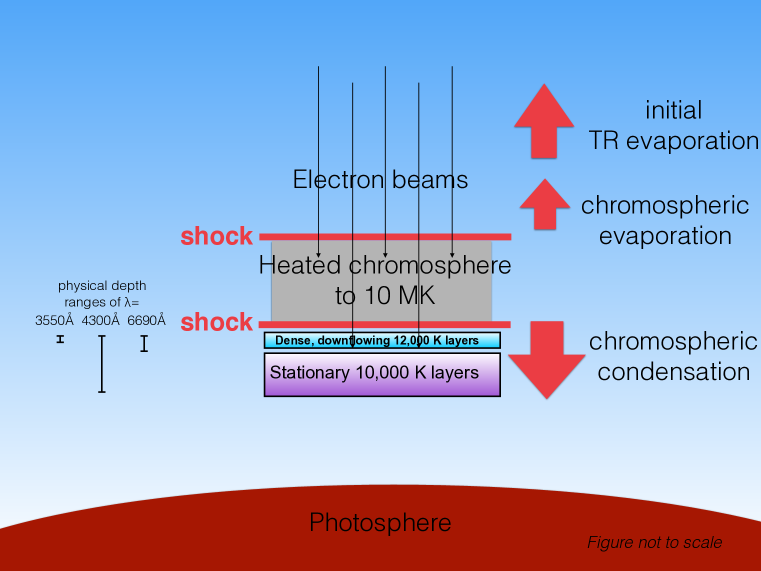
In this talk, we consider the atmospheric response of an M dwarf to a nonthermal electron beam with a constant energy flux of erg cm-2 s-1 (F13) and a double power-law distribution with a minimum (cutoff) energy of 37 keV. The simulation was calculated with the RADYN (Carlsson & Stein, 1997) and RH (Uitenbroek, 2001) codes, and is described in detail in K15. The F13 beam produces two hydrodynamic shocks in the mid to upper chromosphere, and the thermal pressure from these shocks drives material upward (chromospheric evaporation) and downward (chromospheric condensation, hereafter “CC”). The flare atmosphere is illustrated in Figure 1.
The NUV and optical continuum radiation originates from the CC with densities as high as cm-3 and from non-moving (hereafter, the “stationary”) dense ( cm-3) layers below the CC. The CC and stationary layers are indicated in Figure 1; the large number of low-energy electrons in the F13 beam ( keV) is responsible for the rapid heating of the upper chromosphere to MK, which occurs within a short time after helium is completely ionized. The higher energy beam electrons ionize and heat the lower atmospheric heights (the CC and stationary flare layers).
The properties of the surface flux distribution at s are consistent with the impulsive phase constraints from the spectral flare atlas of Kowalski et al. (2013). The F13 surface flux distribution exhibits a Balmer jump ratio (the ratio of NUV continuum to blue continuum flux) of 2 and a color temperature at NUV wavelengths ( Å) and at blue-optical wavelengths ( Å) of K, which are typical properties of observed impulsive phase spectra. In contrast, an F11 model (also considered in K15) exhibits a Balmer jump ratio of and a color temperature of K at blue-optical wavelengths.
To determine the origin of the emergent intensity (and thus the surface flux) at all continuum wavelengths, we use the atmospheric parameters from RADYN to calculate the contribution function, , to the emergent intensity:
| (1) |
which is the total continuum emissivity () at a given height and frequency multiplied by the attenuation of the radiation (determined by ) as it propagates outward in the direction of . The continuum optical depth is obtained by integrating the total continuum opacity () over height. The NLTE spontaneous bound-free (b-f) emissivity and b-f opacity corrected for stimulated emission (Equations 7-1 and 7-2 of Mihalas, 1978) are calculated using the NLTE populations computed in RADYN for a six-level hydrogen atom. Other continuum transitions (involving higher levels of hydrogen, H-, and metals111Although the population of H- is not considered in the equation of radiative transfer and level population equation, its population density is calculated from the NLTE densities of electrons and neutral hydrogen atoms.) are calculated in LTE, as done internally in RADYN. We also consider the NLTE opacity and emissivity from induced recombination, Thomson scattering, and Rayleigh scattering.
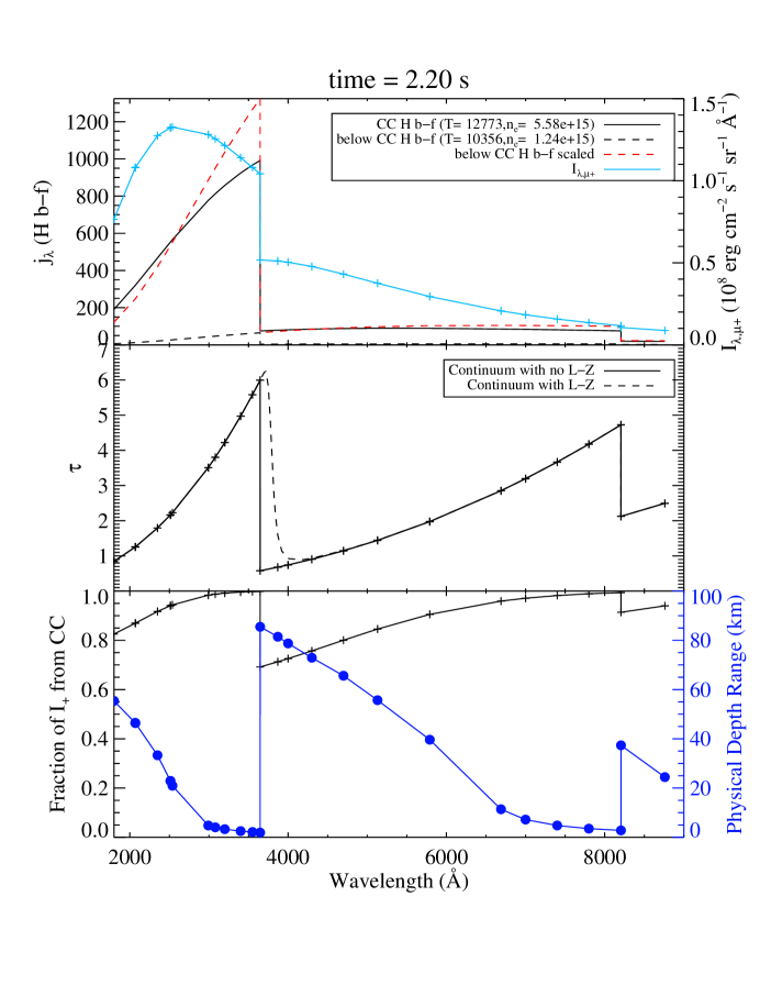
The emissivity and optical depth vary as a function of wavelength and depth in the atmosphere and thus lead to the properties of the spectral energy distribution of the emergent intensity. The dominant emissivity in this model is spontaneous hydrogen Balmer and Paschen recombination emissivity, with lesser (but non-negligible) contributions from hydrogen free-free (f-f) and induced hydrogen recombination. The NLTE spontaneous hydrogen b-f emissivity spectra for representative layers in the CC and the stationary flare layers are shown in the top panel of Figure 2. In the middle panel, we show the total continuum optical depth () at the bottom of the CC (where the downward-directed gas speed decreases below 5 km s-1). Hydrogen has large population densities in the and levels in the CC, which leads to optical depths of nearly at blue wavelengths and optical depths at NUV and red wavelengths. The optical depth variation reflects the hydrogenic b-f cross-section variation.
The emergent intensity spectrum (blue curve in top panel of Figure 2) can be understood as the integral of the contribution function (Equation 1) over height where the emissivity at each height is exponentially attenuated by the optical depth. The hydrogen b-f emissivity spectrum decreases quickly in the NUV, has a large Balmer jump ratio, and has a relatively flat spectrum between the blue (4000 Å) and red (6690 Å) wavelengths. Between recombination edges, the wavelength dependence of the hydrogen b-f emissivity (in units of erg cm-3 s-1 sr-1 Å-1) is proportional to , and the color temperature of the emissivity is related to the emissivity ratio at two wavelengths (through Equation 3 of K15). The color temperature is K for optically thin hydrogen recombination emission at K, and K would also correspond to the color temperature of the emergent intensity if the hydrogen b-f emissivity (e.g., either emissivity curve in the top panel of Figure 2) originates only from layers with low optical depth. Due to the large optical depths and the wavelength dependent variation of the optical depth in the CC (middle panel of Figure 2), the attenuation, given by , multiplies by the top panel222The other non-negligible emissivities from H f-f and H induced b-f are first added to the H spontaneous b-f emissivity. and results in the modified spectral energy distribution of the emergent intensity compared to the spectral energy distribution of the emissivity.
Both the condensation and stationary flare layers contribute to the spectral energy distribution of the emergent spectrum. However, only the blue wavelengths (e.g., Å) are (semi)transparent in the stationary flare layers because these wavelengths have the lowest optical depths. Other wavelengths become opaque in the CC. The fraction of the emergent intensity that originates from the chromospheric condensation is shown in the bottom panel of Figure 2): about 25% of the blue continuum radiation originates in the stationary layers below the CC. Although the emissivity (top panel) is relatively low in these layers because of the lower electron density, the stationary flare layers have a larger vertical extent and the integration of the contribution function over height gives a large value. We compare the transparency of photons using a physical depth range, . The (normalized) cumulative contribution function is given as
| (2) |
where is the emergent intensity and is the height variable (the height variable is defined as at ; Mm corresponds to the top of the model corona). Here we define the physical depth range333In K15, the physical depth range of the CC was calculated as the FHWM of the contribution function within the CC. as the height difference between and . The value of thus defines the height range over which the majority of the emergent intensity is formed.
In Figure 2 (bottom), we show the physical depth range as a function of wavelength. For wavelengths in the NUV (3550Å), blue (4300Å), and red (6690Å), the physical depth ranges are , 72, and 11 km, respectively. These are indicated qualitatively as vertical bars in Figure 1, which illustrates that the physical depth range of blue light extends to the stationary layers, whereas the physical depth ranges of the opaque wavelengths are confined to the CC. The larger transparency of blue photons leads to more photons that can escape from the deeper layers, thus increasing the blue emergent intensity relative to the NUV and red intensities. For a similar reason, the larger transparency of Å NUV photons compared to Å NUV photons produces the ratio of the emergent intensities (apparent from the light blue curve in the top panel of Figure 2) that gives a hot color temperature at wavelengths Å. At Å, the spontaneous hydrogen b-f emissivity rapidly decreases (top panel of Figure 2) and the larger physical depth range at these wavelengths is not large enough to compensate, which results in a peak and turnover towards shorter wavelengths in the emergent intensity spectrum. The physical depth range variation of hydrogen b-f (and f-f) emissivity thus produces an apparently hot color temperature of K and a smaller Balmer jump ratio than are characteristic of optically thin hydrogen recombination radiation.
The Balmer jump ratio and the color temperature of the continuum at the blue and red wavelength sides of the Balmer jump are the result of large optical depths of the continuum emission. Surprisingly, the values of the color temperature of the continuum is not a priori the temperature of the emitting plasma. However, the large optical depths directly result from atmospheric temperatures between K, which produces large thermal populations in the and levels of hydrogen.
2.1 Opacities from Landau-Zener Transitions
Using the RH code, we included the opacity effects from Landau-Zener transitions of electrons within hydrogen atoms with upper energy levels that overlap. The modeling technique is employed in state-of-the art white dwarf model atmosphere codes (Tremblay & Bergeron, 2009). Perturbations from an electric microfield due to ambient charge density perturbs the highest energy levels of hydrogen, which is the Stark effect. At a critical microfield value (which is determined by the proton density; Hummer & Mihalas, 1988), the highest Stark state of an upper level of hydrogen will overlap with the lowest Stark state of , and all levels are “dissolved”. As a result, bound-bound opacity is transferred to b-f opacity via a reverse cascade of electrons that undergo Landau-Zener transitions among the dissolved upper levels. Opacity effects are produced near the Balmer edge because the highest energy levels are most easily perturbed and the energy separation converges for the upper principal quantum states. The modifications to the opacities resulting from Landau-Zener transitions give Balmer recombination emission at wavelengths longer than the Balmer edge and results in a continuous transition from Balmer to Paschen continuum opacity (and emissivity).
The Landau-Zener bound-free opacity at Å is the Balmer continuum opacity extrapolated longward of the Balmer edge which is then multiplied by the dissolved fraction, (Dappen et al., 1987). This opacity is added to the total continuum opacity longward of the Balmer edge. The resulting continuum optical depth at the bottom of the CC is shown as the dashed line in the middle panel of Figure 2; the wavelength extent of the extrapolation of the Balmer opacity longward of the edge () is related to the ambient proton density in the flare atmosphere (see Figure 9 of K15). The maximum ambient proton density attained in the F13 atmosphere is cm-3, and thus Å. The Landau-Zener transitions decrease the bound-bound opacity for transitions with dissolved upper levels, which causes the flux of the highest order Balmer lines to fade into the Balmer continuum emission that is produced redward of Å. Thus, the bluest Balmer line in emission is also related to the ambient proton density. In the F13 model at s, the bluest identifiable Balmer line is H10 or H11, which is similar to some impulsive phase spectra of dMe flares (Kowalski et al., 2013; García-Alvarez et al., 2002); in other flares however, the H15 and H16 lines have been detected (Hawley & Pettersen, 1991; Fuhrmeister et al., 2008; Kowalski et al., 2010).
3 Future Modeling Work
The F13 beam model reproduces the observed continuum flux ratios and the continuum properties within the complicated spectral region near the Balmer edge. These spectral properties can thus be used to infer the physical properties of the flare plasma: continuum flux ratios (the Balmer jump ratio and the color temperature of the continuum) can be used to infer the optical depth, and the wavelength extent of continuum redward of the Balmer jump – or the relative intensity of a higher order Balmer line (H11-H16) – can be used to infer the charge density of the continuum-emitting layers.
In Kowalski et al. (2013), the instantaneous s F13 model was compared to time-resolved spectra during a large flare on the dM4.5e star YZ CMi; agreement between the model and observations was found in the mid rise-phase spectrum. The burst-averaged spectrum (over the 5 s simulation) gives a more direct comparison to the observations, and was in better agreement with the early rise phase or the early gradual decay phase spectra. In future models, the persistence of bright continuum emission needs to be extended for longer times using a sequence of flare bursts in order to be consistent with the observed timescales of white-light flares, which can persist for hours.
The generation of CC’s has long thought to be an important aspect of the standard solar flare model, which includes the precipitation of electrons into the chromosphere producing explosive mass motions (Livshits et al., 1981; Fisher et al., 1985a, b; Fisher, 1989; Gan et al., 1992). The role of chromospheric condensations in solar and M dwarf flares is supported by observed redshifts in the chromospheric lines of H (Ichimoto & Kurokawa, 1984; Canfield et al., 1990) and Mg ii (Graham & Cauzzi, 2015) and the transition region lines of Si iv and C iv (Hawley et al., 2003). Thus, the origin of the white-light continuum in stellar flares in CC’s (and the stationary layers just below) allows us to place this enigmatic phenomenon in the context of the standard solar flare model, albeit with a larger energy flux than usually considered for solar flares. Beam fluxes ranging from erg cm-2 s-1 were also considered in K15, but these fluxes (keeping all else the same as the F13 beam parameters) produce an unsatisfactory match to the observed continuum and emission line flux ratio properties.
We note that the F13 model predicts redshifted, broad chromospheric emission lines, such as H. Though there are only a few high-time resolution observations of M dwarf flares around H with sufficient spectral resolution to infer mass motions, these typically show blueshifts of several tens of km s-1 in the impulsive phase (Hawley et al., 2003; Fuhrmeister et al., 2008).
A number of improvements will be made to our radiative-hydrodynamic flare modeling. First, the F13 beam experiences significant energy loss from a return current electric field, which is discussed in K15. In future models, we will incorporate the energy loss from the return current electric field into the updated RADYN flare code (Allred et al., 2015) and compare to the continuum emission produced by the F13 beam in K15. We will also consider an M dwarf flare model with a higher low-energy cutoff in the electron energy distribution, which mitigates return current effects. We plan to implement an improved prescription for Stark broadening using the Vidal et al. (1973) theory in place of the analytic approximations that are currently used (see K15 for discussion). Thus, we will rigorously determine if charge densities attained in M dwarf flares are as high as cm-3. Future observations with high cadence echelle flare spectra around the Balmer jump and H can provide critical constraints for the formation of such dense CC’s in M dwarf flares. If high density CC’s are formed in M dwarf flares, then we may need to consider a physical mechanism, such neutral beams (Karlický et al., 2000), re-acceleration processes (Varady et al., 2014), or in-situ chromospheric acceleration (Fletcher & Hudson, 2008), to allow F13 beams to penetrate into the lower atmosphere.
4 Implications for Superflares
Recently, superflares in rapidly rotating G stars have been observed with Kepler, revealing energies in the white-light continuum of erg (Maehara et al., 2012; Shibayama et al., 2013; Maehara et al., 2015). These energies are comparable to or even larger than the largest flares observed in M dwarf stars (Hawley & Pettersen, 1991; Osten et al., 2010; Kowalski et al., 2010; Schmidt et al., 2014; Drake et al., 2014). Thus, the energy and duration of the white-light superflares in G stars pose a similar challenge for flare models. Recently, lower nonthermal electron beam energy fluxes of erg cm-2 s-1 have been used to model the areal extent of the white-light emission in superflares (Katsova & Livshits, 2015), but NUV/optical spectra during a superflare would be invaluable for determining if higher energy fluxes are necessary. These spectra would provide new constraints on the color temperature, the Balmer jump ratio, and the properties of the highest order Balmer lines to be directly compared to flare spectra of M dwarf flares. Despite the large peak luminosities, superflares in G stars produce a low contrast against the background emission. Therefore, obtaining high signal-to-noise flare spectra (such as those obtained during a flare on the early type K dwarf AB Doradus from Lalitha et al. (2013)) will be an important observational challenge in the future.
Acknowledgments
AFK thanks the organizers of IAUS #320 for the opportunity to present this work. AFK thanks S. Hawley, K. Shibata, L. Fletcher, G. Cauzzi, and P. Heinzel for stimulating discussions at IAUS #320. AFK acknowledges travel support from HST GO 13323 from the Space Telescope Science Institute, operated by the Association of Universities for Research in Astronomy, Inc., under NASA contract NAS 5-26555, and for travel support from the International Astronomical Union.
References
- Allred et al. (2006) Allred, J. C., Hawley, S. L., Abbett, W. P., & Carlsson, M. 2006, ApJ, 644, 484
- Allred et al. (2015) Allred, J. C., Kowalski, A. F., & Carlsson, M. 2015, ApJ, 809, 104
- Canfield et al. (1990) Canfield, R. C., Penn, M. J., Wulser, J.-P., & Kiplinger, A. L. 1990, ApJ, 363, 318
- Carlsson & Stein (1997) Carlsson, M., & Stein, R. F. 1997, ApJ, 481, 500
- Dappen et al. (1987) Dappen, W., Anderson, L., & Mihalas, D. 1987, ApJ, 319, 195
- Donati-Falchi et al. (1985) Donati-Falchi, A., Falciani, R., & Smaldone, L. A. 1985, A&A, 152, 165
- Doyle et al. (1988) Doyle, J. G., Butler, C. J., Bryne, P. B., & van den Oord, G. H. J. 1988, A&A, 193, 229
- Drake et al. (2014) Drake, S. A., Osten, R. A., Page, K. L., et al. 2014, in AAS/High Energy Astrophysics Division, Vol. 14, AAS/High Energy Astrophysics Division, # 404.06
- Fisher (1989) Fisher, G. H. 1989, ApJ, 346, 1019
- Fisher et al. (1985a) Fisher, G. H., Canfield, R. C., & McClymont, A. N. 1985a, ApJ, 289, 434
- Fisher et al. (1985b) —. 1985b, ApJ, 289, 414
- Fletcher & Hudson (2008) Fletcher, L., & Hudson, H. S. 2008, ApJ, 675, 1645
- Fuhrmeister et al. (2008) Fuhrmeister, B., Liefke, C., Schmitt, J. H. M. M., & Reiners, A. 2008, A&A, 487, 293
- Gan et al. (1992) Gan, W. Q., Rieger, E., Zhang, H. Q., & Fang, C. 1992, ApJ, 397, 694
- García-Alvarez et al. (2002) García-Alvarez, D., Jevremović, D., Doyle, J. G., & Butler, C. J. 2002, A&A, 383, 548
- Graham & Cauzzi (2015) Graham, D. R., & Cauzzi, G. 2015, ApJ, 807, L22
- Gritsyk & Somov (2014) Gritsyk, P. A., & Somov, B. V. 2014, Astronomy Letters, 40, 499
- Hawley & Fisher (1992) Hawley, S. L., & Fisher, G. H. 1992, ApJS, 78, 565
- Hawley & Pettersen (1991) Hawley, S. L., & Pettersen, B. R. 1991, ApJ, 378, 725
- Hawley et al. (2003) Hawley, S. L., Allred, J. C., Johns-Krull, C. M., et al. 2003, ApJ, 597, 535
- Holman et al. (2003) Holman, G. D., Sui, L., Schwartz, R. A., & Emslie, A. G. 2003, ApJ, 595, L97
- Hummer & Mihalas (1988) Hummer, D. G., & Mihalas, D. 1988, ApJ, 331, 794
- Ichimoto & Kurokawa (1984) Ichimoto, K., & Kurokawa, H. 1984, Sol. Phys., 93, 105
- Karlický et al. (2000) Karlický, M., Brown, J. C., Conway, A. J., & Penny, G. 2000, A&A, 353, 729
- Katsova & Livshits (2015) Katsova, M. M., & Livshits, M. A. 2015, Sol. Phys., arXiv:1508.00254
- Kowalski et al. (2015) Kowalski, A. F., Hawley, S. L., Carlsson, M., et al. 2015, Sol. Phys., arXiv:1503.07057
- Kowalski et al. (2010) Kowalski, A. F., Hawley, S. L., Holtzman, J. A., Wisniewski, J. P., & Hilton, E. J. 2010, ApJ, 714, L98
- Kowalski et al. (2013) Kowalski, A. F., Hawley, S. L., Wisniewski, J. P., et al. 2013, ApJS, 207, 15
- Krucker et al. (2011) Krucker, S., Hudson, H. S., Jeffrey, N. L. S., et al. 2011, ApJ, 739, 96
- Lalitha et al. (2013) Lalitha, S., Fuhrmeister, B., Wolter, U., et al. 2013, A&A, 560, A69
- Livshits et al. (1981) Livshits, M. A., Badalian, O. G., Kosovichev, A. G., & Katsova, M. M. 1981, Sol. Phys., 73, 269
- Lovkaya (2013) Lovkaya, M. N. 2013, Astronomy Reports, 57, 603
- Maehara et al. (2015) Maehara, H., Shibayama, T., Notsu, Y., et al. 2015, Earth, Planets, and Space, 67, 59
- Maehara et al. (2012) Maehara, H., Shibayama, T., Notsu, S., et al. 2012, Nature, 485, 478
- Mihalas (1978) Mihalas, D. 1978, Stellar atmospheres /2nd edition/
- Milligan et al. (2014) Milligan, R. O., Kerr, G. S., Dennis, B. R., et al. 2014, ApJ, 793, 70
- Osten et al. (2010) Osten, R. A., Godet, O., Drake, S., et al. 2010, ApJ, 721, 785
- Schmidt et al. (2014) Schmidt, S. J., Prieto, J. L., Stanek, K. Z., et al. 2014, ApJ, 781, L24
- Shibayama et al. (2013) Shibayama, T., Maehara, H., Notsu, S., et al. 2013, ApJS, 209, 5
- Tremblay & Bergeron (2009) Tremblay, P.-E., & Bergeron, P. 2009, ApJ, 696, 1755
- Uitenbroek (2001) Uitenbroek, H. 2001, ApJ, 557, 389
- Varady et al. (2014) Varady, M., Karlický, M., Moravec, Z., & Kašparová, J. 2014, A&A, 563, A51
- Vidal et al. (1973) Vidal, C. R., Cooper, J., & Smith, E. W. 1973, ApJS, 25, 37
- Zarro & Zirin (1985) Zarro, D. M., & Zirin, H. 1985, A&A, 148, 240
- Zhilyaev et al. (2007) Zhilyaev, B. E., Romanyuk, Y. O., Svyatogorov, O. A., et al. 2007, A&A, 465, 235