Delay times in chaotic quantum systems

Abstract

By an inductive reasoning, and based on recent results of the joint moments of proper delay times of open chaotic systems for ideal coupling to leads, we obtain a general expression for the distribution of the partial delay times for an arbitrary number of channels and any symmetry. This distribution was not completely known for all symmetry classes. Our theoretical distribution is verified by random matrix theory simulations of ballistic chaotic cavities.

I Introduction

The delay experienced by a quantum particle due to the interaction with a scattering region has been the subject of intense investigation for more than thirty years in several areas that include nuclear and condensed matter physics.Wigner ; Smith ; Lyuboshits ; Bauer ; Landauer ; Price ; Iannaccone The interest in this subject has resurged due to the recent appearance of theoretical investigations in chaotic systemsBerkolaiko ; Mezzadri1 ; Mezzadri2 ; Kuipers ; Marciani ; Novaes1 ; Novaes2 and atomic physics;Feist2014 ; Ivanov2014 ; Deshmukh2014 ; Chacon2014 the later motivated by experiments of interaction of light with matter during a mean time with attosecond precision.Schultze2010

The delay time first introduced by WignerWigner for one channel and its multichannel generalization by Smith,Smith in the so-called Wigner-Smith time delay matrix, is written in terms of the scattering matrix $S$ and its derivative with respect to the energy $\varepsilon$. In units of the Heisenberg time $\tau_{{}_{\rm{H}}}$, it is given by

$$Q_{{}_{\rm{W}}}=-\mathrm{i}\frac{\hbar}{\tau_{{}_{\rm{H}}}}S^{-1}\frac{\partial S}{\partial\varepsilon}.$$ (1)

The eigenvalues of $Q_{{}_{\rm{W}}}$ represent the delay time on each channel and the Wigner time delay is the average of these proper delay times. In the context of mesoscopic systems the electrochemical capacitance of a mesoscopic capacitor is described by the Wigner time delay.Lambe ; Buttiker1 ; Buttiker2 Some other transport observables that depend on the proper delay times are the thermopower,vanLangen the derivative of the conductance with respect to the Fermi energy,BrouwerdG the DC pumped current at zero bias,BrouwerPumping among others (see for instance Ref. BrouwerWRM, and references there in). For ballistic systems with chaotic classical dynamics, these physical observables fluctuates with respect small variations of external parameters, like an applied magnetic field, the Fermi energy or the system shape,FyodorovJMP ; Frahm1 ; BrouwerWRM the proper delay times are of interest in the characterization of their universal statistics. The distribution of the proper delay times is given in terms of the joint distribution of their reciprocals, known as the Laguerre ensemble,Frahm1 ; BrouwerWRM which depends on the particular symmetry present in the problem; an interesting feature of this ensemble is the presence of level repulsion, as occur in the spectral statistics of several complex quantum-mechanical systems.

Alternatively, the partial delay times defined as the energy derivative of phase shifts are also useful in the characterization of chaotic scattering.FyodorovJMP Although the partial times are correlated, this correlation is of different nature than that between the proper delay times; they do not show the level repulsion.Savin In the one channel situation the proper an partial delay times are identical to the Wigner time delay $\tau$ whose distribution is known for all symmetry classes:FyodorovJMP ; Gopar ; FyodorovPRE55 $\beta=1$ (4) in the presence of time reversal and presence (absence) of spin-rotation symmetry, and $\beta=2$ in the absence of time reversal symmetry. For the general case of arbitrary number of channels, the distribution of a partial time is known for $\beta=2$FyodorovPRL76 ; Seba and for $\beta=1$ an expression in terms of quadratures was obtained for non-ideal coupling.FyodorovPRE55 In the ideal coupling case only the tails of the distribution are known and the corrected prediction does not seem to be right.Seba Moreover, the $\beta=4$ symmetry is seldom discussed and the distribution of partial times for this symmetry class is not given yet.

In the present paper, we obtain, by an inductive reasoning, a general expression for the probability distribution of the partial delay times. This was done by extracting the essence that comes from the level repulsion in the joint distribution of proper delay times, that transcends to the $k$th moment of a proper delay time.Angeljmp We test our formula by random matrix theory simulations for all symmetry classes and for several number of channels.

In the next section we establish the theoretical framework of the proper and partial delay times; we review the known results for the $k$th moment of a proper delay time from which we obtain a general expression of the probability distribution of the partial times, for all symmetry classes and any number of channels. In Sect. III we compare our generalized distribution with the numerical predictions from random matrix theory. We conclude in Sect. IV.

II Distributions of proper and partial delay times

II.1 Scattering approach

Single-electron scattering by a ballistic cavity attached ideally to two leads which support $N_{1}$ and $N_{2}$ propagating modes (channels), respectively, can be described by a $N\times N$ scattering matrix $S$, where $N=N_{1}+N_{2}$. When the dynamics of the cavity is classically chaotic, the scattering matrix belongs to one of the three circular ensembles of random matrix theory (RMT).Mehta ; Dyson The circular unitary ensemble (CUE) is obtained when flux conservation is the only restriction in the problem, such that $S^{\dagger}S=\openone_{N}$, where $\openone_{N}$ denotes de unit matrix of dimension $N$. In the Dyson scheme this case is labeled by $\beta=2$. Additionally, in the presence of time reversal invariance (TRI) and integral spin or TRI, half-integral spin and rotation symmetry, $S$ is a symmetric matrix, $S=S^{T}$ (the upper script $T$ means transpose). This case is denoted by $\beta=1$ and the corresponding ensemble is the circular orthogonal ensemble (COE). In the presence of TRI, half-integral spin, and no rotation symmetry, $S$ is self-dual and the ensemble of self-dual scattering matrices is the circular symplectic ensemble (CSE), labeled by $\beta=4$. In the diagonal form, the $S$ matrix can be written as

$$S=UEU^{\dagger},$$ (2)

where $U$ is a $N\times N$ unitary, the matrix of eigenvectors, and $E$ is the diagonal matrix of eigenphases,

$$E_{ij}=\mathrm{e}^{\mathrm{i}\theta_{i}}\,\delta_{ij},$$ (3)

with $\delta_{ij}$ the Kronecker delta.

II.2 Proper delay times

A symmetrized form of the Wigner-Smith time delay matrix can be written in dimensionless units asFrahm1 ; BrouwerWRM

$$Q=-\mathrm{i}\frac{\hbar}{\tau_{{}_{\rm{H}}}}\,S^{-1/2}\frac{\partial S}{\partial\varepsilon}S^{-1/2},$$ (4)

where $\varepsilon$ is the energy and $\tau_{{}_{\rm{H}}}$ is the Heisenberg time ($\tau_{{}_{\rm{H}}}=2\pi\hbar/\Delta$, with $\Delta$ the mean level spacing). The matrix $Q$ is Hermitian for $\beta=2$, real symmetric for $\beta=1$, and quaternion self-dual for $\beta=4$. Its eigenvalues, $q_{i}$’s ($i=1,\,\ldots,\,N$) are the proper delay times measured in units of $\tau_{{}_{\rm{H}}}$. The distribution of the $q_{i}$’s in terms of their reciprocals $x_{i}=1/q_{i}$ is given by the Laguerre ensembleFrahm1

$$p_{\beta}(\{x_{i}\})=C_{N}^{(\beta)}\prod_{a<b}^{N}\left|x_{b}-x_{a}\right|^{\beta}\prod_{c=1}^{N}x_{c}^{\beta N/2}\,\mathrm{e}^{-\beta x_{c}/2},$$ (5)

where $C_{N}^{(\beta)}$ is a normalization constant. It is worth mentioning that the level repulsion that appears between the proper delay times is inherited of the Hamiltonian eigenvalues. There, its normalization constant is well known;Guhr however, the constant $C_{N}^{(\beta)}$ has not been given yet, although the Laguerre distribution has been widely used. Through the analysis given in Ref. Angeljmp, we find a general expression given by

$$C^{(\beta)}_{N}=\frac{\left[\left(\frac{\beta}{2}\right)^{\beta(N-1/2)+1}\left(\frac{\beta}{2}\right)!\right]^{N}}{\left(\frac{\beta N}{2}\right)!}\prod_{n=0}^{2N-1}\frac{1}{\left(\frac{\beta n}{2}\right)!}\,.$$ (6)

Let us note that the level repulsion of the proper delay times in (5) transcends to the $k$th moment of them; recent results of that $k$th moment, valid for any symmetry and an arbitrary number of channels, shows the underlying part that comes from this repulsion, namelyAngeljmp

$$\left\langle q_{i}^{k}\right\rangle^{(\beta)}=\left(\frac{\beta}{2}\right)^{k}\frac{\left(\frac{\beta N}{2}-k\right)!}{\left(\frac{\beta N}{2}\right)!}\,K_{N}^{(\beta)}(k,0,\ldots,0),$$ (7)

for $k<1+\beta N/2$. The factor $K_{N}^{(\beta)}(k,0,\ldots,0)$ is the inheritance part of the level repulsion according to the above statement. For $k=1$, 2, and 3 it becomes independent of $\beta$,Angeljmp

$$K_{N}^{(\beta)}(k,0,\ldots,0)=\frac{k!N^{k-1}N!}{(N+k-1)!}.$$ (8)

II.3 Partial delay times

Partial delay times, defined as the energy derivative of the diagonal form of the scattering matrix as in Eq. (1), are given, in dimensionless units, byFyodorovJMP ; Seba

$$\hat{\tau}=-\mathrm{i}\frac{\hbar}{\tau_{{}_{\rm{H}}}}E^{-1}\frac{\partial E}{\partial\varepsilon}.$$ (9)

It is an $N\times N$ diagonal matrix with elements

$$\tau_{s}=\frac{\hbar}{\tau_{{}_{\rm{H}}}}\frac{\partial\theta_{s}}{\partial\varepsilon}.$$ (10)

Since the partial delay times dot not show level repulsion, once the inherent part of the level repulsion has been identified, it is easy to arrive at the expression of the $k$th moment of the partial time, that isAngeljmp

$$\left\langle\tau_{s}^{k}\right\rangle^{(\beta)}=\left(\frac{\beta}{2}\right)^{k}\frac{\left(\frac{\beta N}{2}-k\right)!}{\left(\frac{\beta N}{2}\right)!},$$ (11)

This expression is in agreement with the results that can be obtained directly from the distributionGopar for the $N=1$ case and any $\beta$. Also, Eq. (11) is in agreement with the known result for $\beta=2$ and arbitrary $N$.FyodorovJMP ; FyodorovPRL76 Following this inductive line of thought, we arrive at the distribution of the partial delay times for all symmetry classes and any number of channels, namely

$$P_{\beta}(\tau_{s})=\frac{2/\beta}{\left(\frac{\beta N}{2}\right)!}\,\left(\frac{\beta}{2\tau_{s}}\right)^{2+\beta N/2}\mathrm{e}^{-\beta/2\tau_{s}}.$$ (12)

This is our main result in this paper. Our expression encompasses the existing results in the literature.Gopar ; FyodorovPRE55 ; FyodorovJMP ; FyodorovPRL76 ; Seba

In what follows we verify our finding with random matrix theory simulations.

III Numerical calculations

The Hamiltonian approach, also known as the Heidelberg approach, is the best suited for the calculation of the energy derivative of the scattering matrix since it is written explicitly in terms of the energy, namely Guhr ; Verbaarschot ; BeenakkerRMP

$$S(\varepsilon)=\openone_{N}-2{\rm i}\pi W^{\dagger}\frac{1}{\varepsilon\openone_{M}-H+{\rm i}\pi WW^{\dagger}}W,$$ (13)

where $H$ is an $M$-dimensional Hamiltonian matrix that describes the chaotic dynamics of the system, with $M$ resonant single-particle states, and $W$ is a $M\times N$ matrix, independent of the energy, which couples these resonant states with the $N$ propagating modes in the leads; $\openone_{n}$ stands for the unit matrix of dimension $n$. For ideal coupling of uncorrelated equivalent channels, $W_{\mu n}=\sqrt{M\Delta}/\pi$ ($\mu=1,\,\ldots,\,M$ and $n=1,\,\ldots,\,N$) for the matrix elements of $W$.BeenakkerRMP

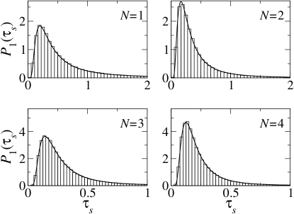
Figure 1: Comparison between the numerical simulations (histograms) and theory (continuous lines), Eq. (12), for the distribution of $\tau_{s}$ (we take $s=1$) in the $\beta=1$ case.

For chaotic systems, $H$ is a random matrix chosen from one of the Gaussian ensembles: orthogonal ($\beta=1$), unitary ($\beta=2$) or symplectic ($\beta=4$). The matrix elements of $H$ are uncorrelated random variables with a Gaussian probability distribution with zero mean and variance $\lambda^{2}/\beta M$; the later determines the mean level spacing at the center of the band, $\Delta=\pi\lambda/M$.Guhr An ensemble of Hamiltonian matrices leads to an ensemble of $S$-matrices, which represents the several realizations of systems for which the statistical analysis is performed. To implement the simulations we followed the same method as in Ref. Mucciolo, for $\beta=1$ and 2, while for $\beta=4$ the subroutine given in Ref. Cappellini, was used to generate the random Hamiltonian.

For each realization we diagonalize the matrix $S$ to determine its eigenvalues. We are interested in one of the eigenvalues only, $E_{s}(\varepsilon)=\exp[\mathrm{i}\theta_{s}(\varepsilon)]$ let say, but evaluated at three energies in order to calculate the energy derivative. That is,

$$\tau_{s}=-\frac{\mathrm{i}}{2\pi\epsilon}\,\frac{E_{s}(\epsilon/2)-E_{s}(-\epsilon/2)}{E_{s}(0)},$$ (14)

where $\epsilon=\varepsilon/\Delta$.

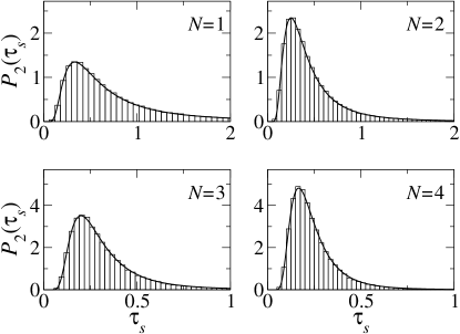
Figure 2: The same as in Fig. 1 but for $\beta=2$.

In Fig. 1 we compare our theoretical distribution for the partial delay times, Eq. (12), for $\beta=1$, with the numerical results obtained from the random matrix simulations with $10^{5}$ realizations of $\tau_{s}$, calculated as in Eq. (14) for $M=100$ and $\epsilon=0.001$. We observe an excellent agreement for the several cases of $N$ presented. This result is an important one since it has not been verified before. Figure 2 shows the corresponding results for $\beta=2$, which is in agreement those of Ref. Seba, . For $\beta=4$ the comparison is shown in Fig. 3 where also we observe an excellent agreement. Let us note that this is the first time that the distribution of the partial times is given and verified for the $\beta=4$ and any number of channels.

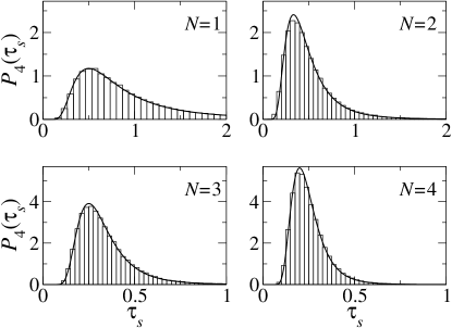
Figure 3: The same as in Fig. 1 but for $\beta=4$.

IV Conclusions

Based on known results of the joint moments of proper delay times, we obtained the distribution of the partial delay times for an arbitrary number of channels and any symmetry. This was done following and inductive method by extracting the underlying part coming from the level repulsion inherited to the $k$th moment of a proper delay time. Our distribution not only reproduces theoretical results previously considered in the literature for unitary symmetry, but also extends it to the orthogonal and symplectic symmetries, for an arbitrary number of channels. Besides, we were able to provide the normalization constant for the joint distribution of proper delay times. We tested our theoretical distribution by random matrix theory simulations of ballistic chaotic cavities with ideal coupling.

- (1) E. P. Wigner, Phys. Rev. 98 145 (1955).
- (2) F. T. Smith, Phys. Rev. 118, 349 (1960).
- (3) L. Lyuboshits, Phys. Lett. B 72, 41 (1977).
- (4) M. Bauer, P. A. Mello, and K. W. McVoy, Z. Phys. A 293, 151 (1979).
- (5) R. Landauer and Th. Martin, Rev. Mod. Phys. 66, 217 (1994).
- (6) P. J. Price, Phys. Rev, B 48, 17301 (1993).
- (7) G. Iannaccone, Phys. Rev. B 51, 4727 (1995).
- (8) G. Berkolaiko and J. Kuipers, J. Phys. A: Math. Theor. 43, 035101 (2010).
- (9) F. Mezzadri and N. J. Simm, J. Math. Phys. 52, 103511 (2011).
- (10) F. Mezzadri and N. J. Simm, J. Math. Phys. 53, 053504 (2012).
- (11) J. Kuipers, D. V. Savin, and M. Sieber, New J. Phys. 16, 123018 (2014).
- (12) M. Marciani, P. W. Brouwer, and C. W. J. Beenakker, Phys. Rev B 90, 045403 (2014).
- (13) M. Novaes, J. Math. Phys. 56, 062110 (2015).
- (14) M. Novaes, J. Math. Phys. 56, 062109 (2015).
- (15) J. Feist, O. Zatsarinny, S. Nagele, R. Pazourek, J. Burgdörfer, X. Guan, K. Bartschat, and B. I. Schneider, Phys. Rev. A 89, 033417 (2014).
- (16) I. A. Ivanov and A. S. Kheifets, Phys. Rev. A 89, 043405 (2014).
- (17) P. C. Deshmukh, A. Mandal, S. Saha, A. S. Kheifets, V. K. Dolmatov, and S. T. Manson, Phys. Rev. A 69, 053424 (2014).
- (18) A. Chacon, M. Lein, and C. Ruiz, Phys. Rev. A 89, 053427 (2014).
- (19) M. Schultze, M. Fie, N. Karpowicz, J. Gagnon, M. Korbman, M. Hofstetter, S. Neppl, A. L. Cavalieri, Y. Komninos, Th. Mercouris, C. A. Nicolaides, R. Pazourek, S. Nagele, J. Feist, J. Burgdörfer, A. M. Azzeer, R. Ernstorfer, R. Kienberger, U. Kleineberg, E. Goulielmakis, F. Krausz, and V. S. Yakovlev, Science 328, 1658 (2010).
- (20) J. Lambe and R. C. Jaklevic, Phys. Rev. Lett. 22, 1371 (1969).
- (21) M. Büttiker, J. Phys.: Condens. Matter 5, 9361 (1993).
- (22) M. Büttiker, A. Prêtre, and H. Thomas, Phys. Rev. Lett. 70, 4114 (1993).
- (23) S. A. van Langen, P. G. Silvestrov, and C. W. J. Beenakker, Superlatt. Microstruct. 23, 691 (1998).
- (24) P. W. Brouwer, S. A. van Langen, K. M. Frahm, M. Büttiker, and C. W. J. Beenakker, Phys. Rev. Lett. 79, 913 (1997).
- (25) P. W. Brouwer, Phys. Rev. B 58, R10135 (1998).
- (26) P. W. Brouwer, K. M. Frahm, and C. W. J. Beenakker, Waves Random Media 9, 91 (1999).
- (27) Y. V. Fyodorov and H.-J. Sommers, J. Math. Phys. 38, 1918 (1997).
- (28) P. W. Brouwer, K. M. Frahm, and C. W. J. Beenakker, Phys. Rev. Lett. 78, 4737 (1997).
- (29) D. V. Savin, Y. V. Fyodorov, and H.-J. Sommers, Phys. Rev. E 63, 035202(R), (2001).
- (30) V. A. Gopar, P. A. Mello, and M. Büttiker, Phys. Rev. Lett. 77, 3005 (1996).
- (31) Y. V. Fyodorov, D. V. Savin, and H.-J. Sommers, Phys. Rev. E. 55, R4857 (1997).
- (32) Y. V. Fyodorov and H.-J. Sommers, Phys. Rev. Lett. 76, 4709 (1996).
- (33) P. Šeba, K. Życzkowski, and J. Zakrzewski, Phys. Rev. E 54, 2438 (1996).
- (34) A. M. Martínez-Argüello, M. Martínez-Mares, and J. C. García, J. Math. Phys. 55, 081901 (2014).
- (35) M. L. Mehta, Random Matrices (Academic, New York, 1991).
- (36) F. J. Dyson, J. Math. Phys. (N.Y.) 3, 140 (1962).
- (37) T. Guhr, A. Müller-Groeling, and H. A. Weidenmüller, Phys. Rep. 299, 189 (1998).
- (38) J. J. M. Verbaarschot, H. A. Weidenmüller, and M. R. Zirnbauer, Phys. Rep. 129, 367 (1985).
- (39) C. W. J. Beenakker, Rev. Mod. Phys. 69, 731 (1997).
- (40) M. Martínez-Mares, C. H. Lewenkopf, and E. R. Mucciolo, Phys. Rev. B 69, 085301 (2004).
- (41) V. Cappellini’s home page at http://users.ictp.it/valerio/HTML/ForTran/RMT.html.