Abstract

The linear sigma model with linearized fluctuations of all involved fields facilitates the onset of a sequence of first-order phase transitions at a critical point. This phase structure has distinctive imprints on the photon emission rates. We argue that analogously a critical point in the QCD phase diagram manifests itself by peculiarities of the photon spectra, in particular when the dynamical expansion path of matter crosses the phase transition curve in the vicinity of the critical point.
PACS12.39.Fe – 13.60.-r – 13.60.Fz – 11.30.Qc

1 Introduction

The conjecture that QCD displays a non-trivial phase diagram has triggered a series of dedicated investigations. On the experimental side, the beam energy scan at RHIC has brought up some remarkable results [1] which are under discussion w.r.t. an interpretation in terms of the onset of deconfinement at lower beam energies. It is supported by earlier observations of particular features seen in the beam energy dependence of selected observables, most notably the ”horn” in the $K^{+}/\pi^{+}$ ratio [2]. On the theoretical side, lattice QCD thermodynamic quantities have proven that the transition to deconfined matter at zero chemical potential occurs in a (rapid) crossover. What remains unsettled is the existence of a first-order phase transition curve $T_{c}(\mu)$ in the temperature ($T$) vs. chemical potential ($\mu$) plane, terminating in a (critical) end point (CEP) at $\mu_{c}>0$. The existence and the location of the CEP, quantified by $T_{c}(\mu_{c})$ and $\mu_{c}$, is a challenging task. With present techniques, ab initio QCD approaches can hardly fix the values of $T_{c}(\mu_{c})$ and $\mu_{c}$ as well as the confinement-deconfinement delineation curve $T_{c}(\mu)$ for $\mu>\mu_{c}$. Various models give widespread results [3, 4].

The planned facilities NICA and FAIR will operate in a range of beam energies which is considered promising for the search of a QCD CEP. For example, the energy range, where the maximum freeze-out densities are achieved [5, 6], will be covered by NICA; it is also just the energy $\sqrt{s_{NN}}=\mathcal{O}(8\,\mathrm{GeV})$ where the above mentioned ”horn” is seen. Since NICA will be equipped with detector installations which enable the measurement of photons, one may ask whether the direct photon spectra have distinctive imprints of a CEP or the emerging first-order phase transition sequence.

To attempt an answer to this question, we are going to employ a particular model with a CEP and calculate, within a kinetic theory approach, a few relevant channels for photon emission of strongly interacting matter in the vicinity of the CEP.

Owing to their penetrating nature, electromagnetic probes (dileptons as well as real photons) are promising tools for investigating the whole evolution of matter in the course of heavy-ion collisions, although the convolution of signals from all stages of the evolution requires some effort in disentangling the respective sources the photons. Especially interesting are the thermal photons from the hydrodynamic expansion stage if the system crosses the phase border line [7, 8]. Thus, understanding the experimental data (see e.g. [9] for a review) requires precise theoretical insight into the production processes (see [10, 11] for transport, [12, 13] for kinetic theory approaches to the thermal photon rates or [14, 15] for recent reviews).

2 A model with CEP: The linear sigma model

The linear sigma model ($\mathrm{L}\sigma\mathrm{M}$) [16, 17, 18, 19] is known to display a CEP as endpoint of a first-order phase transition curve $T_{c}(\mu)$. The degrees of freedom are quarks ($q=(u,d)$) and mesons ($\sigma,\pi^{0,\pm}$). The Lagrangian reads

$$\mathcal{L}_{\mathrm{L}\sigma\mathrm{M}} = \bar{q}(i\not{\partial}-g(\sigma+i\gamma_{5}\bm{\tau}\bm{\pi}))q-\mathcal{L}_{km}-U(\sigma,\bm{\pi}),$$ (1)

$$U(\sigma,\bm{\pi}) = \frac{\lambda}{4}(\sigma^{2}+\bm{\pi}^{2}-\zeta)^{2}-H\sigma,$$ (2)

$$\mathcal{L}_{km} = \frac{1}{2}(\partial_{\mu}\sigma\partial^{\mu}\sigma+\partial_{\mu}\bm{\pi}\partial^{\mu}\bm{\pi}),$$ (3)

where $g$, $\zeta$, $\lambda$ and $H$ are parameters which can be fixed, e.g. by adjustments to nucleon, pion and sigma masses as well as the pion decay constant. For convenience we choose the same parameter fixing as [20, 21], i.e. $g=3.387$, $\zeta=7874\,\mathrm{MeV}^{2}$, $\lambda=27.58$ and $H=1.760\times 10^{6}\,\mathrm{MeV}^{3}$.

The grand potential is given by a path integral of the exponential of the action constructed from $\mathcal{L}_{\mathrm{L}\sigma\mathrm{M}}$. In mean field approximation (MFA) for the meson fields, one replaces the meson fields by their thermal averages, which results in the thermodynamic potential

$$\Omega_{\text{MFA}} = \Omega_{qq}\Big{|}_{m_{q}=gv}+U(v,\bm{0}),$$ (4)

with $\Omega_{qq}$ being the potential constructed from the fermionic part of the Lagrangian and $v$ being the thermal expectation value of the $\sigma$ field. The resulting phase structure based on $\Omega_{\text{MFA}}$ is discussed in [16]. Most important for our purpose is the variation of the effective masses over the phase diagram which is not restricted to the $\mathrm{L}\sigma\mathrm{M}$ but can also be found for other chiral models such as the NJL model [22, 16].

We include here, similar to [20, 21, 23], linearized fluctuations to account for quanta of the meson fields which participate in reactions with photons in the exit channel but exclude vacuum terms for all the fields. In the linearized fluctuation approach (LFA) the fermionic part $\Omega_{qq}$ is calculated first and contributes, via the quark mass $m_{q}=g\sqrt{\sigma^{2}+\pi^{2}}$, to the effective meson potential. This effective potential is afterwards approximated by a parabola leading eventually to

$$\Omega_{\text{LFA}}= \langle U(v+\Delta,\bm{\pi})\rangle+\langle\Omega_{qq}(m_{q})\rangle$$ (5)

$$\quad-\frac{1}{2}m_{\sigma}^{2}\langle\Delta^{2}\rangle-\frac{1}{2}m_{\pi}^{2}\langle\bm{\pi}^{2}\rangle+\Omega_{\pi}+\Omega_{\sigma},$$

where $\sigma=v+\Delta$ and the brackets $\langle f(\sigma,\bm{\pi})\rangle$ denoting the ensemble average of a function $f$ over $\sigma$ and $\pi$ fields and $\Omega_{\sigma,\pi}$ denoting the potential for noninteracting bosons with effective masses $m_{\sigma,\pi}$ and multiplicities 1 and 3, respectively. The emerging phase structure based on $\Omega_{\text{LFA}}$ is discussed in [21, 23, 24] (for full account of fluctuations, cf. [25]), where also the relations to symmetries of two-flavor QCD are recollected.

The chiral transition of the $\mathrm{L}\sigma\mathrm{M}$ belongs to the class of liquid-gas type phase transitions [26], where the entropy per quark $s/n$ displays at the phase boundary a drop both with increasing temperature at constant chemical potential $\mu>\mu_{c}$ or with increasing chemical potential at constant temperature, see Fig. 1.

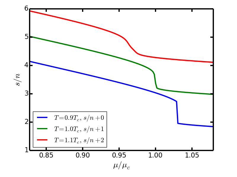
Figure 1: Entropy per quark $s/n$ as a function of scaled chemical potential for the $\mathrm{L}\sigma\mathrm{M}$ in LFA. The ratio is shown for $T>T_{c}$, $T\approx T_{c}$ and $T<T_{c}$ (from top to bottom). For better visibility the upper curves have offsets of 1 and 2. Parameters as in [27, 24] yielding $\mu_{c}=278\,\mathrm{MeV}$ and $T_{c}\equiv T_{c}(\mu_{c})=74\,\mathrm{MeV}$, quite different from values advocated recently in [28] or [25] which are above or below that temperature value.

In general, local stability requires $s_{1}\equiv s(T_{c}^{-})<s_{2}\equiv s(T_{c}^{+})$ and $n_{1}\equiv n(T_{c}^{-})<n_{2}\equiv n(T_{c}^{+})$ at a first-order phase transition. However, whether $s_{1}/n_{1}<s_{2}/n_{2}$ holds (as for the liquid-gas type transition [26]) depends on the details of the equation of state, i.e. the relation of degrees of freedom and latent heat in schematic models. As a consequence, the isentropic curves on which $s/n$ = const may bend upward ($s_{1}/n_{1}>s_{2}/n_{2}$) or downward ($s_{1}/n_{1}<s_{2}/n_{2}$) on the phase border curve $T_{c}(\mu)$, supposed $\partial T_{c}(\mu)/\partial\mu<0$. (For a discussion of isentropes within models superimposing a singular CEP potential and a smooth background in the spirit of condensed matter approaches, cf. [29]). In other words, the phase coexistence curve $p_{c}(T)$ has a positive (negative) slope for the liquid-gas (hadron-quark) type transition, as evidenced by the Clapeyron equation $dp_{c}/dT=(s_{1}/n_{1}-s_{2}/n_{2})/(1/n_{1}-1/n_{2})$. Due to the poor description of baryonic degrees of freedom in the $\mathrm{L}\sigma\mathrm{M}$, one must not trust the behavior at small temperatures. Taken as such it is a specific model with a CEP and the liquid-gas transition type (for a more generic discussion of other models, cf. [31]) with the pattern of isentropic curves as exhibited in Fig. 2. There, the isentrope with $s/n=2.8$ runs slightly below the phase transition line after bypassing the CEP contrary to those with $s/n<2.8$. These join the $T_{c}(\mu)$ curve, run some section along it and depart at a lower ”exit temperature”. Remarkable for the model with the chosen parameters mentioned above is the low value of the temperature at the exit point. For other parameter fixings these exit temperatures can be significantly larger; then also the CEP in absolute $T-\mu$ units changes (see [32, 24] for systematics).

The thermal photon yield is obtained by integrating the photon emission rates along these trajectories from certain ”initial” points (cf. [7, 8] for estimates), where the system produced in a heavy-ion collision can be considered as thermalized, until freeze-out, supposed an adiabatic expansion applies at least approximately.

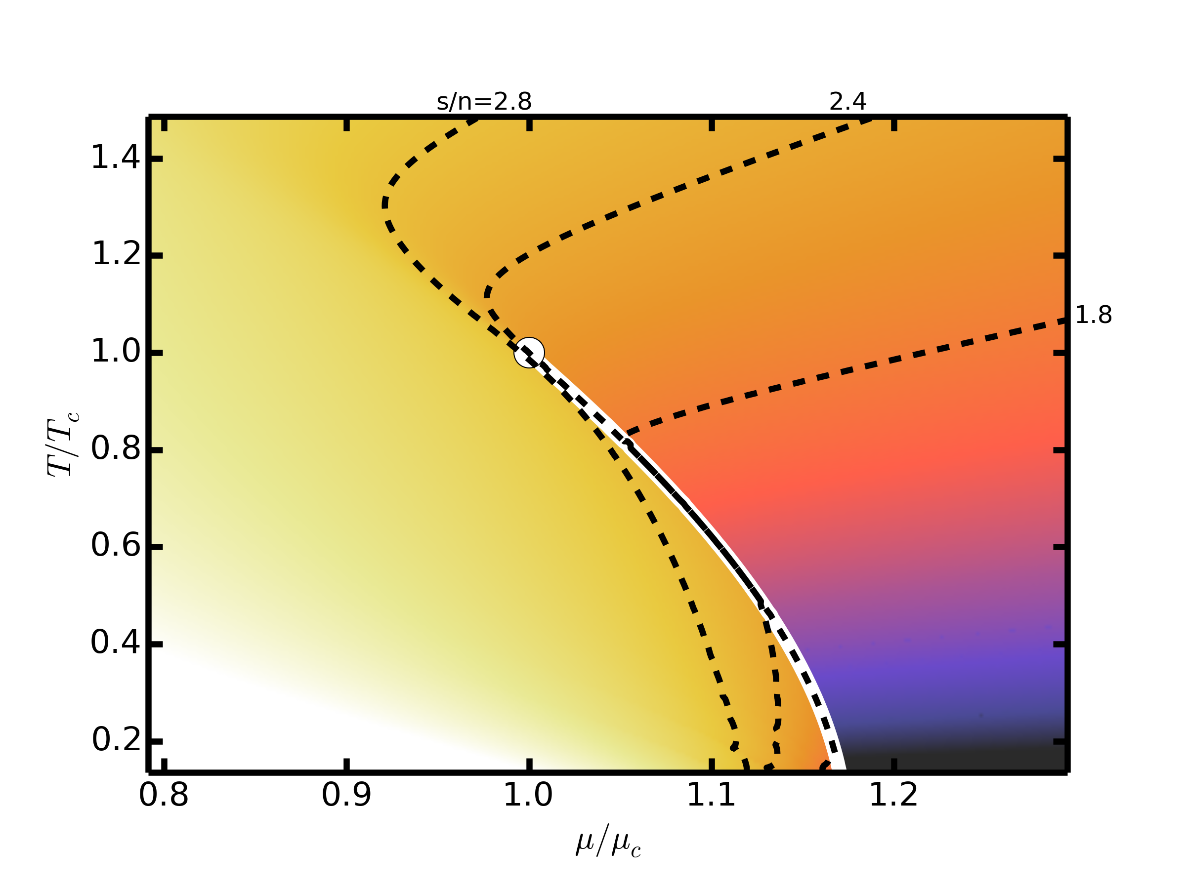
Figure 2: Isentropic curves $s/n$ = const in the scaled $T-\mu$-plane. The first-order phase boundary, depicted by the white curve, terminates in the CEP (white bullet). The dashed white curve is an estimate of the crossover region. Below the phase transition curve the isentropes are ordered from $s/n=2.8$ to $s/n=1.8$ (left to right).

3 Photon emissivities

For calculating photon emission rates, the $\mathrm{L}\sigma\mathrm{M}$ needs to be equipped with an electromagnetic sector. This is done by adding a kinetic term

$$\mathcal{L}_{k\gamma}=\frac{1}{4}F^{\mu\nu}F_{\mu\nu}$$ (6)

and by coupling the photon field with field strength tensor $F^{\mu\nu}$ and four-potential $A^{\mu}$ minimally to quarks and mesons by replacing $\partial_{\mu}\rightarrow\partial_{\mu}+ieQA_{\mu}$ as done, e.g. , in [33] for the NJL model. Considering the fluctuations of the fields $q,\sigma,\bm{\pi}$ as quanta with effective masses $m^{*}_{q,\sigma,\pi}$ and corresponding dispersion relations $E_{i}^{2}={m^{*}_{i}}^{2}+p^{2}$ the following photon-producing binary reactions in lowest order

$$q_{i}+\sigma,\pi \rightarrow q_{j}+\gamma \text{(Compton scatterings off quarks)},$$ (7)

$$\bar{q}_{i}+\sigma,\pi \rightarrow\bar{q}_{j}+\gamma \text{(Compton scat. off antiquarks)},$$ (8)

$$q_{i}+\bar{q}_{j} \rightarrow\sigma,\pi+\gamma$$ (annihilations) (9)

are accessible within a kinetic theory approach yielding the emission rates

$$\omega\frac{d^{7}N_{12\rightarrow 3\gamma}}{dx^{4}dk^{3}}= \,C\int\frac{d^{3}p_{1}}{2p_{1}^{0}}\frac{d^{3}p_{2}}{2p_{2}^{0}}\frac{d^{3}p_{3}}{2p_{3}^{0}}\delta(p_{1}+p_{2}-p_{3}-k)$$ (10)

$$\times|\mathcal{M}_{12\rightarrow 3\gamma}|^{2}f_{1}(p_{1})f_{2}(p_{2})\big{(}1\pm f_{3}(p_{3})\big{)}.$$

Here $f_{i}(p_{i})=n_{F,B}(p_{i}^{0})$ are the Fermi or Bose distribution functions of the involved species, respectively, $\mathcal{M}$ is the corresponding matrix element and $C=(2(2\pi)^{8})^{-1}$ is a normalization factor. In MFA the identification of the effective masses is

$$m^{*}_{q} = gv$$ (11)

$${m^{*}_{\sigma}}^{2} = \frac{\partial^{2}\Omega_{qq}\big{|}_{m_{q}=gv}}{\partial v^{2}}+\lambda(3v^{2}-\zeta),$$ (12)

$${m^{*}_{\pi}}^{2} = 2g^{2}\frac{\partial\Omega_{qq}}{\partial m_{q}^{2}}\Bigg{|}_{m_{q}=gv}+\lambda(v^{2}-\zeta),$$ (13)

$$0 = \frac{\partial\Omega_{qq}\big{|}_{m_{q}=gv}}{\partial v}+\lambda(v^{3}-v\zeta)-H,$$ (14)

with $v$ being the thermal expectation value of the $\sigma$ field, while the linearized fluctuation approach suggests to use

$$m^{*}_{q} = g\left\langle\sqrt{\sigma^{2}+\bm{\pi}^{2}}\right\rangle,$$ (15)

$${m^{*}_{\sigma}}^{2} = \left\langle\frac{\partial^{2}\Omega_{qq}}{\partial\Delta^{2}}\right\rangle+\lambda(3v^{2}+3\langle\Delta^{2}\rangle+\langle\bm{\pi}^{2}\rangle-\zeta),$$ (16)

$${m^{*}_{\pi}}^{2} = \left\langle\frac{\partial^{2}\Omega_{qq}}{\partial\pi_{a}^{2}}\right\rangle+\lambda(v^{2}+\langle\Delta^{2}\rangle+\frac{5}{3}\langle\bm{\pi}^{2}\rangle-\zeta),$$ (17)

$$0 = \left\langle\frac{\partial\Omega_{qq}}{\partial\Delta}\right\rangle+\lambda v(v^{2}+3\langle\Delta^{2}\rangle+\langle\bm{\pi}^{2}\rangle-\zeta)-H,$$ (18)

where the variances of the meson fields have to be determined self consistently via $\langle\Delta^{2}\rangle,\langle\pi_{a}^{2}\rangle=2\partial\Omega_{\sigma,\pi}/\partial(m_{\sigma,\pi_{a}}^{2})$. Thus the effective masses correspond to thermally averaged ”curvature masses” (cf. [34]). The matrix elements squared are calculated according to the Feynman diagrams depicted in Fig. 3.

Figure 3: Lowest-order Feynman diagrams for the processes (7)-(9). The top row shows the diagrams for the Compton processes for quarks and the bottom row those for annihilations. If the meson is a $\sigma$ only the left two columns contribute, because the $\sigma$ does not couple to the photon, but (some of) the pions do.

The rates (10) depend on the photon energy $\omega$ and, via the effective masses, (see Fig. 1 in [27]) on temperature and chemical potential together with the explicit $T$ and $\mu$ dependence of the $f_{i}$. Given the variations of $m_{q,\sigma,\pi}^{*}$ over the phase diagram, the photon emission rates (10) map out the phase structure [27, 24].

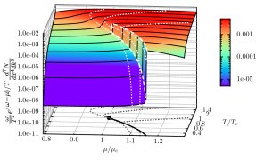
Figure 4: Scaled photon emission rate for $\omega=1\,\mathrm{GeV}$ in the vicinity of the critical point for the Compton process (7) involving $\pi$ mesons. The first-order phase transition curve $T_{c}(\mu)$ and the CEP are depicted in the bottom plane. Black curves at the emission rate surface depict the rate at constant temperature. The dashed white curve surrounds the region where the rate jumps as a consequence of the discontinuity of the masses across the phase border line. The dotted curves are the rates along the $s/n=2.8,2.4,1.8$ (left to right) isentropes also shown at the base of the plot.

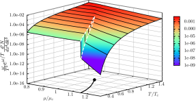
Figure 5: As in Fig. 4 but for the annihilation process (9) involving $\pi$ mesons. The lines correspond to those of Fig. 4; note that the scaling factor differs from the one in Fig. 4.

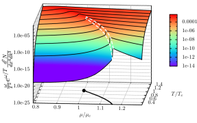
Figure 6: As in Fig. 4 but for the annihilation process (9) involving $\sigma$ mesons. The lines correspond to those of Fig. 4; scaling factor as in Fig. 5.

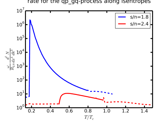
Figure 7: Photon emission rates for the Compton process (7) with pions along the isentropes shown in Fig. 2. The rates are scaled by the rate $R_{2.8}$ along the $s/n=2.8$ isentrope for making the influence of the first-order phase transition apparent. Solid curves depict the scaled rates in the coexistence region.

Selecting $\omega=1\,\mathrm{GeV}$ we exhibit in Figs. 4-6 the emission rates for the reactions (7) (with pions) and (9) (with pions and sigmas). To highlight the variations of the emissivities, we display the scaled rates $T^{-2}\exp\{(\omega-\mu)/T\}\omega d^{7}N_{\gamma}/(dk^{3}dx^{4})$, where the exponential scales out the asymptotic high-energy behavior [24]. Due to the discontinuities of the masses across the phase transition curve, also the rates reflect these peculiarities: Depending on the participating species, the respective rates may jump up as in Figs. 4 and 6 or drop down as in Fig. 5 at the phase boundary when crossing it at constant temperature with increasing chemical potential. The size of the jumps as well as their direction depends mostly on the mass of the outgoing particle (besides the photon). Within a Boltzmann approximation for the distribution functions it can be shown that for large $\omega$ the dominant mass dependence is $\propto\exp\{-m_{3}/T\}$ [24]. Thus, the decrease of the quark and sigma mass (for constant temperature and increasing chemical potential) leads to an increase of the Compton rate (cf. Fig. 4) or the annihilation rate with sigmas (cf. Fig. 6), while an increase of the pion mass leads to a dropping rate in the annihilation case with pions (cf. Fig. 5). The size of the jumps changes from one order of magnitude near the CEP to many orders of magnitude for small $T$ depending also on the process under consideration. Beyond the CEP and the first-order phase transition line the rates vary smoothly over the $T-\mu$-plane.

To arrive at some impression of the variation of the rates along an adiabatic expansion path, we exhibit in Fig. 7 the rates along isentropic trajectories in the vicinity of the phase border curve. The solid curves are for the scaled rates, where the isentropic curve runs on the coexistence curve $T_{c}(\mu)$. Here, the rates are a superposition in the spirit of a two-phase mixture, i.e. $dN=dN_{+}(T^{+}(\mu))x+dN_{-}(T^{-}(\mu))(1-x)$, where x means the weight of the high-temperature phase. (Analog constructions of two-phase mixtures apply for density, entropy density and energy density). The large ratios of the rates depicted in Fig. 7 for the $s/n=1.8$ curve can be understood in terms of phase mixing in the coexistence region. At the phase boundary the photon emission originates from both phases. For the Compton-process the above mentioned leading mass dependence is $\propto\exp\{-m_{q}/T\}$. Because the drop of the quark mass is of order $200\,\mathrm{MeV}$ at small temperatures (cf. Fig. 1c in [27]) the rate in the high-temperature phase is enhanced w.r.t. the low-temperature phase emission rate by a factor of $\exp\{\Delta m_{q}/T\}$ which can achieve values up to $10^{5}$ close to the exit temperature of these isentropes, even for small phase weight of the high-temperature phase. For the rates along the isentropes depicted in Figs. 2 and 4, this means that these curves stay close to the upper rim of the discontinuity even if $T$ is only slightly larger than the above mentioned ”exit temperature” (cf. Fig. 4) and the huge enhancement factor corresponds to a jump of the rates of the same order of magnitude. Despite these huge differences in the emission rates at temperatures considerably smaller than the CEP temperature, the total photon yield is less wide spread, because the major part of the thermal photon emission is from the hot medium with $T>T_{c}(\mu_{c})$, where the isentropic emission rates in Fig. 7 are of the same order of magnitude.

Clearly, besides the $2\rightarrow 2$ processes considered so far, the other channels must be accounted for to arrive at firm conclusions. Nevertheless, these results support the hypotheses that the photon emission may obey distinctive peculiarities when the matter in the course of a heavy-ion collision undergoes a first-order phase transition, supposed it is strong enough.

4 Summary

In summary, we have shown that a few selected channels for the photon emissivity directly map out the phase diagram. Despite of the great progress of ab initio calculations for a variety of quantities characterizing the properties of strongly interacting matter, the region of non-zero baryon density is less reliable accessible in a wide range. Therefore, we resort here to a specific model which displays a critical end point (CEP), where a curve of first-order phase transitions, which are of the liquid-gas type, sets in and continues to larger baryon densities. The considered photon generating processes refer to lowest-order reactions of the involved effective degrees of freedom. For the corresponding rates a crucial ingredience is represented by the so-called derivative masses which obey significant variations, or even discontinuities, in the vicinity of the critical endpoint, causing a strong imprint on the rates. Clearly, the consideration of many more channels along with improved inclusion of QCD like degrees of freedom is necessary to arrive at realistic estimates of the total emission rate. Equally challenging is also the account of the dynamics (cf. [35] for a method to follow the smoothed longitudinal evolution of matter or [26] for the treatment of spinodal clumping in the mixed phase). Nevertheless, we hope that our explorative investigations have digged out pertinent features of modifications of penetrating probes monitoring the evolution of matter in the course of heavy-ion collisions in the energy range of NICA. Guided by the experience from macroscopic examples of critical point phenomena, e.g. critical opalescence emerging from a diverging correlation length in approaching the CEP, one would expect more drastic signatures, e.g. related to a strong spike in the specific heat or a stall/push of the expansion dynamics, which in turn would shape the space-time integrated photon spectra. In our approach, however, the CEP imprints on the net-photon emission rate is rather modest due to the solely coupling to the derivative masses of effective degrees of freedom.

5 Acknowledgments

One of the authors (BK) gratefully acknowledges useful conversations with J. Randrup on the relation of liquid-gas and hadron-quark transitions. The work is supported by BMBF grant 05P12CRGH.

References

- [1] D. McDonald, EPJ Web Conf. 95, 01009 (2015).
- [2] S. V. Afanasiev et al., Phys. Rev. C66, 054902 (2002).
- [3] M. A. Stephanov, Prog. Theor. Phys. Suppl. 153, 139 (2004).
- [4] B. Friman et al., editors, The CBM physics book: Compressed baryonic matter in laboratory experiments, volume 814 of Lect. Notes Phys., Springer, Berlin, 2011.
- [5] J. Randrup and J. Cleymans, Phys. Rev. C74, 047901 (2006).
- [6] J. Randrup and J. Cleymans, arXiv:0905.2824 [nucl-th] (2009).
- [7] E. L. Bratkovskaya et al., Phys. Rev. C69, 054907 (2004).
- [8] Yu. B. Ivanov, V. N. Russkikh, and V. D. Toneev, Phys. Rev. C73, 044904 (2006).
- [9] I. Tserruya, Landolt-Börnstein 23, 176 (2010).
- [10] B. Bäuchle and M. Bleicher, Phys. Rev. C82, 064901 (2010).
- [11] O. Linnyk, W. Cassing, and E. L. Bratkovskaya, Phys. Rev. C89, 034908 (2014).
- [12] W. Liu and R. Rapp, Nucl. Phys. A796, 101 (2007).
- [13] H. van Hees, C. Gale, and R. Rapp, Phys. Rev. C84, 054906 (2011).
- [14] C. Gale, Landolt-Börnstein 23, 445 (2010).
- [15] R. Rapp, J. Wambach, and H. van Hees, Landolt-Börnstein 23, 134 (2010).
- [16] O. Scavenius, A. Mocsy, I. Mishustin, and D. Rischke, Phys. Rev. C64, 045202 (2001).
- [17] B.-J. Schaefer and J. Wambach, Nucl. Phys. A757, 479 (2005).
- [18] B.-J. Schaefer, J. M. Pawlowski, and J. Wambach, Phys. Rev. D76, 074023 (2007).
- [19] T. K. Herbst, J. M. Pawlowski, and B.-J. Schaefer, Phys. Lett. B696, 58 (2011).
- [20] A. Mocsy, I. Mishustin, and P. Ellis, Phys. Rev. C70, 015204 (2004).
- [21] E. S. Bowman and J. I. Kapusta, Phys. Rev. C79, 015202 (2009).
- [22] D. Blaschke, D. Zablocki, M. Buballa, A. Dubinin, and G. Röpke, Annals Phys. 348, 228 (2014).
- [23] L. Ferroni, V. Koch, and M. B. Pinto, Phys. Rev. C82, 055205 (2010).
- [24] F. Wunderlich and B. Kämpfer, to be published in PoS CPOD2014 (2015).
- [25] R.-A. Tripolt, N. Strodthoff, L. von Smekal, and J. Wambach, Phys. Rev. D89, 034010 (2014).
- [26] J. Steinheimer, J. Randrup, and V. Koch, Phys. Rev. C89, 034901 (2014).
- [27] F. Wunderlich and B. Kämpfer, J. Phys. Conf. Ser. 599, 012019 (2015).
- [28] R. A. Lacey, Phys. Rev. Lett. 114, 142301 (2015).
- [29] M. Bluhm and B. Kämpfer, PoS CPOD2006, 004 (2006).
- [30] R. Schulze and B. Kämpfer, arXiv:0912.2827 [nucl-th] (2009).
- [31] M. Hempel, V. Dexheimer, S. Schramm, and I. Iosilevskiy, Phys. Rev. C88, 014906 (2013).
- [32] B.-J. Schaefer and M. Wagner, Phys. Rev. D79, 014018 (2009).
- [33] K. Fukushima, M. Ruggieri, and R. Gatto, Phys. Rev. D81, 114031 (2010).
- [34] A. J. Helmboldt, J. M. Pawlowski, and N. Strodthoff, Phys. Rev. D91, 054010 (2015).
- [35] F. Wunderlich and B. Kämpfer, Eur. Phys. J. A48, 169 (2012).