Scenario generation for single-period portfolio selection problems with tail risk measures: coping with high dimensions and integer variables

Abstract

In this paper we propose a problem-driven scenario generation approach to the single-period portfolio selection problem which use tail risk measures such as conditional value-at-risk. Tail risk measures are useful for quantifying potential losses in worst cases. However, for scenario-based problems these are problematic: because the value of a tail risk measure only depends on a small subset of the support of the distribution of asset returns, traditional scenario based methods, which spread scenarios evenly across the whole support of the distribution, yield very unstable solutions unless we use a very large number of scenarios. The proposed approach works by prioritizing the construction of scenarios in the areas of a probability distribution which correspond to the tail losses of feasible portfolios.

The proposed approach can be applied to difficult instances of the portfolio selection problem characterized by high-dimensions, non-elliptical distributions of asset returns, and the presence of integer variables. It is also observed that the methodology works better as the feasible set of portfolios becomes more constrained. Based on this fact, a heuristic algorithm based on the sample average approximation method is proposed. This algorithm works by adding artificial constraints to the problem which are gradually tightened, allowing one to telescope onto high quality solutions.

1 Introduction

In the portfolio selection problem one must decide how to invest in a collection of financial instruments with uncertain returns which in some way balances portfolio return against risk. There are many ways of modeling this problem. In the robust optimization setting, the returns of the portfolio are assumed to fall within some uncertainty set, and one minimizes the worst-case of loss [BT06]. This approach is sometimes considered too conservative as it does not make effective use of available information. In stochastic programming, the user uses their knowledge and available data to explicitly model asset returns as random vectors, and then optimize some combination of expected return and risk measure. In between these two paradigms is distributionally-robust optimization [HZFF10] where the returns are modeled by a random vector whose distribution lies in some uncertainty set, and the worst-case expected loss is minimized. This approach is particularly useful when only limited or unreliable data is available to model the uncertainty, but can lead to intractable problems. Besides the optimization paradigm employed, portfolio selection problems can be further categorized into single-period problems, where only one portfolio selection is made, and multiperiod problems where the portfolio may be rebalanced several times.

The work in this paper applies to the stochastic programming single-period formulation of the portfolio selection problem. This approach is popular as it allows one to flexibly model the return of the distributions, can easily incorporate problem details such as transactions costs [LFB07], while remaining generally more tractable than other types of models. We deal in particular with a difficult variety of this problem type which involve tail risk measures and potentially integer variables.

In the typical set-up the uncertain returns are modeled by random variables, the total return of a portfolio is some linear combination of these, and riskiness is measured by a real-valued function of the total return which should in some way penalize potential large losses. This approach was first proposed by Markowitz [Mar52] who used variance as a risk measure.

Although the use of variance has remained popular [LFB07] because it leads to tractable convex programs, its use as a measure of risk is problematic for a few reasons. The foremost of these is perhaps that variance penalizes large profits as well as large losses. As a consequence, in the case where the returns of financial assets are not normally distributed, using the variance can lead to potentially bad decisions; for instance, a portfolio can be chosen in favor of one which always has higher returns (see [You98] for an example of this). This particular issue can be overcome by using a “downside” risk measure, that is one which only depends on losses greater than the mean, or some other specified threshold, for example the semi-variance [Mar59, Chapter 9], mean regret [DR99], or value-at-risk [Jor96]. More recently, much research has been given to coherent risk measures, a concept introduced in [ADEH99]. These are risk measures which have sensible properties such as subadditivity, which in particular ensures that a risk measure incentivizes diversification of a portfolio. Using a coherent risk measure in a portfolio selection problem should avoid flawed decisions, such as the one cited in the case of variance.

In this work, we are interested in portfolio selection problems involving tail risk measures. These can be thought of as risk measures which only depend on the upper tail of a distribution above some specified quantile. A canonical example of a tail risk measure is the value-at-risk (VaR) [Jor96]. The $\beta$-VaR is defined to be the $\beta$-quantile of a random variable. In portfolio selection problems this has the appealing interpretation as the amount of capital required to cover up to $\beta\times 100\%$ of potential losses. Thus, tail risk measures, in particular those which dominate the $\beta\operatorname{-VaR}$, are useful as they can give us some idea of the amount capital at risk in the worst $(1-\beta)\times 100\%$ of potential losses. Like variance, the value-at-risk is also problematic as it is not a coherent measure of risk. Specifically, it is not subadditive (see [Tas02] for example). Moreover, $\beta\operatorname{-VaR}$ leads to difficult and intractable problems when used in an optimization context. The conditional value-at-risk (CVaR), sometimes referred to as the expected shortfall, is another tail risk measure and can be roughly thought as the conditional expectation of a random variable above the $\beta$-VaR. It is both coherent [AT02], and more tractable in an optimization setting [RU00].

However, the use of risk measures, even coherent ones such as $\beta\operatorname{-CVaR}$, is still problematic in portfolio selection problems where the asset returns are modeled with continuous probability distributions. This is because the evaluation of many risk measures for arbitrary continuously distributed returns would involve the evaluation of a multidimensional integral, and this becomes computationally infeasible when our problems involve many assets. On the other hand, the evaluation of such an integral reduces to a summation if the returns have a discrete distribution.

Scenario generation is the construction of a finite discrete distribution to be used in a stochastic optimization problem. This may involve fitting a parametric model to asset returns and then discretizing this distribution, or directly modeling them with a discrete distribution, for example via moment-matching [HKW03]. In either case, standard scenario generation methods struggle to adequately represent the uncertainty in problems using tail risk measures. This is because the value of a tail risk measure, by definition, only depends on a small subset of the support of a random variable, and typical scenario generation methods will spread their scenarios evenly across the whole support of the distribution. This means that the region on which the value of the tail risk depends, is represented by relatively few scenarios. Hence, unless there is a very large number of scenarios, the value of of tail risk measure is very unstable (see [KWVZ07] for example).

The natural remedy to this problem is to represent the regions of the distribution on which the tail risk measure depends with more scenarios. Intuition would tell us that these correspond to the “tails” of the distribution. However, for a multivariate distribution there is no canonical definition of the tails. If by tails, we simply mean the region where at least one of the components exceeds a large value, then the probability of this region quickly converges to one with the problem dimension, and thus prioritizing scenarios in this region will be of little benefit. Finding the relevant tails of the distribution is a non-trivial problem.

In our previous paper [FTW17] we addressed the problem of scenario generation for stochastic programs with an arbitrary loss function functions which use tail risk measures, and for this we defined the concept of a $\beta$-risk region. In portfolio selection, to each valid portfolio there is a distribution of losses (or returns). The $\beta$-risk region consists of all potential asset returns which lead to a loss in the $\beta$-tail for some portfolio. We have shown that under mild conditions the value of a tail risk measure in effect only depends on the distribution of returns in the risk region. Although characterizing this region in a convenient way is generally not possible, we have been able to do this for the portfolio selection problem when the asset returns are elliptically distributed. We have also proposed a sampling approach to scenario generation using these risk regions which prioritizes the generation of scenarios in the risk region. We demonstrated for simple examples that this methodology can produce scenario sets which yield better and more stable solutions than does basic sampling.

In this paper we address issues related to the application of this methodology to realistic portfolio selection problems. The first major contribution of this work is the application of the methodology to problems where the asset returns have non-elliptical distributions. In this case the distribution of returns for a portfolio will in general not have a convenient closed form, and so it is necessary to represent the asset returns with a scenario set. In order to apply the methodology, we approximate the risk region for a non-elliptical distribution with the risk region of an elliptical distribution. Moreover, we demonstrate that the methodology is effective on difficult problems which have high dimensions and integer variables.

In the paper [FTW17] it was shown that our methodology is more effective as the problem becomes more constrained. The second major contribution of this work is the proposal of an heuristic algorithm based on the stochastic average approximation (SAA) method [KSHdM01] which exploits this fact. This algorithm works by adding artificial constraints to the problem which are gradually tightened, allowing one to telescope onto high quality solutions. This algorithm is presented in a general way and could be potentially used on problems other than portfolio selection.

The paper is organized as follows. In Section 2 we formally define risk regions for general stochastic programs, and present some new results on the use of approximate risk regions. In Section 3 we define the portfolio selection problem and recall some results on the use of the risk region methodology for this problem. We also provide some new technical results related exploiting risk regions of elliptical distributions. In Section 4 we describe how risk regions are exploited for the purpose of scenario generation, and present a heuristic based on the SAA method based which uses of artificial constraints. In Section 5 we make some empirical observations on how the probability of the non-risk region, a quantity which determines the effectiveness of the methodology, varies with the type of distribution of asset returns. In Section 6 we present results for a broad range of numerical tests on the effectiveness of our sampling and reduction algorithm using distributions constructed from real asset return data. In Section 7 we demonstrate the performance of the proposed heuristic on a difficult case study problem. Finally, in Section 8 we make some concluding remarks.

2 Risk regions for general stochastic programs

In this section we formally define the concept of risk region and present results related to these. This theory does not just apply to portfolio selection problems but more generally to stochastic programs with a tail risk measure. In Section 2.1 we recall the basic definitions and fundamental results for risk regions which appeared in our previous paper [FTW17]. In Section 2.2 we present some new results related to the approximation of risk regions.

2.1 Tail risk measures and risk regions

A risk measure is a function of a real-valued random variable representing a loss. For $0<\beta\leq 1$, a $\beta$-tail risk measure can be thought of as a function of a random variable which depends only on the upper $(1-\beta)$-tail of the distribution. The precise definition uses the generalized inverse distribution function or (lower) quantile function.

Definition 2.1 (Quantile function and $\beta$-tail risk measure).

Suppose $Z$ is a random variable with distribution function $F_{Z}$. Then the generalized inverse distribution function, or quantile function is defined as follows:

$$F^{-1}_{Z}:(0,1] \rightarrow\mathbb{R}\cup\{\infty\}$$

$$\beta \mapsto\inf\{z\in\mathbb{R}:F_{Z}(x)\geq\beta\}$$

Now a $\beta$-tail risk measure is any function of a random variable, $\rho_{\beta}(Z)$, which depends only on the quantile function of a random variable above $\beta$.

Example 2.2 (Value at risk (VaR)).

Let $Z$ be a random variable, and $0<\beta<1$. Then, the $\beta-$VaR for $Z$ is defined to be the $\beta$-quantile of $Z$:

$$\beta\operatorname{-VaR}(Z):=F_{Z}^{-1}(\beta)$$

.

Example 2.3 (Conditional value at risk (CVaR)).

Let $Z$ be a random variable, and $0<\beta<1$. Then, the $\beta\operatorname{-CVaR}$ can be thought roughly as the conditional expectation of a random variable above its $\beta$-quantile. The following alternative characterization of $\beta\operatorname{-CVaR}$ [AT02] shows directly that it is a $\beta$-tail risk measure.

$$\beta\operatorname{-CVaR}(Z)=\int_{\beta}^{1}F^{-1}_{Z}(u)\ du$$

The observation that we exploit for this work is that very different random variables will have the same $\beta$-tail risk measure as long as their $\beta$-tails are the same.

In the optimization context we suppose that the loss depends on some decision $x\in\mathcal{X}\subseteq\mathbb{R}^{k}$ and the outcome of some latent random vector $Y$ with support $\mathcal{Y}\subseteq\mathbb{R}^{d}$, defined on a probability space $(\Omega,\mathcal{F},\mathbb{P})$, and which is independent of $x$. That is, we suppose our loss is determined by some function, $f:\mathcal{X}\times\mathbb{R}^{d}\rightarrow\mathbb{R}$, which we refer to as the loss function. For a given decision $x\in\mathcal{X}$, the random variable associated with the loss is thus $f(x,Y)$.

To avoid repeated use of cumbersome notation we introduce the following short-hand for distribution and quantile functions:

$$F_{x}(z) :=F_{f(x,Y)}(z)=\mathbb{P}\left(f(x,Y)\leq z\right),$$

$$F_{x}^{-1}(\beta) :=F_{f(x,Y)}^{-1}(\beta)=\inf\{z\in\mathbb{R}:\ F_{x}(z)\geq\beta\}.$$

In [FTW17] we introduced the concept of a risk region for a stochastic program using a tail-risk measure. We define this now for a general stochastic program.

Definition 2.4 (Risk region).

The $\beta$-risk region associated associated with the random vector $Y$ and the feasible region $\mathcal{X}\subseteq\mathbb{R}^{d}$ is as follows:

$$\mathcal{R}_{Y,\mathcal{X}}(\beta):=\bigcup_{x\in\mathcal{X}}\{y\in\mathbb{R}^{d}:\ f(x,y)\geq F^{-1}_{x}\left(\beta\right)\}.$$ (1)

The risk region consists precisely of those outcomes of $Y$ which have a loss in the $\beta$-tail of the loss distribution for some feasible decision. We refer to the complement of the risk region as the non-risk region and this consists of outcomes which never lead to a loss in the $\beta$-tail; it can be written as follows:

$$\mathcal{R}_{Y,\mathcal{X}}(\beta)^{c}=\bigcap_{x\in\mathcal{X}}\{y\in\mathbb{R}^{d}:f(x,y)<F_{x}^{-1}(\beta)\}.$$ (2)

The following theorem was proved in [FTW17] and states that under mild conditions the value of a tail risk measure is completely determined by the the distribution of the random vector $Y$ in the risk region. That is, the values of the tail risk measure of any two random vectors with identical distributions in the risk region will be the same for all feasible decisions. The technical condition in (3), which we call the aggregation condition for reasons explained below, precludes certain degenerate cases. In essence, this condition ensures that there is enough mass in the set to ensure that the $\beta$-quantile does not depend on the probability distribution outside of it.

Theorem 2.5.

Let $\mathcal{R}\supseteq\mathcal{R}_{Y,\mathcal{X}}(\beta)$ be such that for all $x\in\mathcal{X}$ the following condition holds:

$$\mathbb{P}\left(Y\in\{y:z^{\prime}<f(x,y)\leq F_{x}^{-1}\left(\beta\right)\}\cap\mathcal{R}\right)>0\qquad\forall\ z^{\prime}<F^{-1}_{x}\left(\beta\right).$$ (3)

If $\tilde{Y}$ is a random vector for which the following holds:

$$\mathbb{P}\left(Y\in\mathcal{A}\right)=\mathbb{P}\left(\tilde{Y}\in\mathcal{A}\right)\qquad\text{for any }\mathcal{A}\subseteq\mathcal{R},$$ (4)

then $\rho_{\beta}\left(f(x,Y)\right)=\rho_{\beta}\left(f(x,\tilde{Y})\right)$ for all $x\in\mathcal{X}$, for any $\beta$-tail risk measure $\rho_{\beta}$.

With regards to scenario generation, this theorem says that any scenarios in the non-risk region can be aggregated into a single point, reducing the size of the problem, without affecting the value of the tail risk measure. This motivates the term aggregation condition for (3). The transformed random vector where all mass in a region has been concentrated into its conditional expectation plays a special role in this work. We call this the aggregated random vector.

Definition 2.6 (Aggregated Random Vector).

For some set $\mathcal{R}\supseteq\mathcal{R}_{Y,\mathcal{X}}$ the aggregated random vector is defined as follows:

$$\psi_{\mathcal{R}}(Y):=\begin{cases}Y&\text{if }Y\in\mathcal{R},\\ \mathbb{E}\left[\ Y|Y\in\mathcal{R}^{c}\ \right]&\text{otherwise.}\end{cases}$$

The conditional expectation $\mathbb{E}\left[\ Y|Y\in\mathcal{R}^{c}\ \right]$ is guaranteed to fall in the non-risk region if, for example, the loss function is convex [FTW17, Proposition 3].

2.2 Approximation of Risk Regions

The methodology proposed in this paper requires a characterization of a risk region which allows one to easily test membership. A convenient characterization for the exact risk region as defined in (1) is in general not possible as this set is determined by the loss function, distribution of the random vector and the problem constraints. Even for the portfolio selection which has a simple loss function, we cannot find a convenient form for arbitrary distributions of asset returns.

Recall that Theorem 2.5 applies to any set containing the risk region. Therefore, one way to circumvent the problem of finding the exact risk region would be to use a conservative risk region, that is, a set which contains the exact risk region. This approach is particularly useful for problems which have constraints which cannot be easily taken into account, such as constraints involving integer variables in the portfolio selection problem. By Definition 2.4, if $\mathcal{X}\subseteq\mathcal{X}^{\prime}$ then $\mathcal{R}_{Y,\mathcal{X}}\subseteq\mathcal{R}_{Y,\mathcal{X}^{\prime}}$. Therefore, ignoring some constraints will yield a risk region which is conservative.

In the case where one cannot construct a risk region for a given loss function or distribution, it may be difficult to find a conservative risk region. Moreover, it could be the case that a conservative risk region may be too conservative to be of any use. Instead one might try to use an approximate risk region. For the portfolio selection problem we handle distributions for which we cannot conveniently characterize the exact risk region by using the risk region of a surrogate distribution which is similar to the true distribution.

Denote by $\mathcal{R}\subset\mathbb{R}^{d}$ an approximate risk region. When using an approximate risk region the value of the tail risk measure may be distorted for a decision $x\in\mathcal{X}$ if $\mathcal{R}$ does not contain all outcomes in the $\beta$-tail, that is, unless the following condition holds:

$$\sup_{y\in\mathcal{R}^{c}}f(x,y)\leq F^{-1}_{x}(\beta).$$ (5)

If (5) holds then we say that that the approximate risk region $\mathcal{R}$ is valid for decision $x$.

We show in this section that if the approximate risk region is not valid for a particular decision, then, under mild assumptions, the values of $\beta\operatorname{-VaR}$ and $\beta\operatorname{-CVaR}$ tail risk measures are distorted downwards. In Section 3, we will exploit this observation to show that for the problems in which we are interested, if there is no distortion of the value of the tail risk measure at the optimal solution, then this solution is also optimal with respect to the true problem.

For the results in this section we employ the following notation: $\hat{F}_{x}$ and $\hat{F}^{-1}_{x}$ denote respectively the distribution and quantile functions of $\psi_{\mathcal{R}}(Y)$. We require the following conditions:

1. $z\mapsto F_{x}(z)$ is continuous for all $x\in\mathcal{X}$

2. $\mathbb{E}\left[Y|Y\in\mathcal{R}^{c}\right]\in\mathcal{R}_{Y,\mathcal{X}}^{c}$

Assumption (B) requires that conditional expectation of $Y$ in the complement of approximate risk region belongs to the exact non-risk region. This means that the loss at the aggregated point will have a loss below the $\beta$-quantile of $f(x,Y)$ for all feasible decisions $x\in\mathcal{X}$. Before stating and proving the key result, we require the following lemma.

Lemma 2.7.

Under assumptions (A) and (B), the approximate distribution function $\hat{F}_{x}$ is continuous for all $x\in\mathcal{X}$ at $z$ for ${z>f\left(x,\mathbb{E}\left[Y|Y\in\mathcal{R}\right]\right)}$.

Proof.

Fix $x\in\mathcal{X}$ and $z>f\left(x,\mathbb{E}\left[Y|Y\in\mathcal{R}\right]\right)$, and without loss of generality assume that ${f\left(x,\mathbb{E}\left[Y|Y\in\mathcal{R}\right]\right)<z^{\prime}<z}$. Now,

$$\hat{F}_{x}(z)-\hat{F}_{x}(z^{\prime}) =\mathbb{P}\left(f(x,\psi_{\mathcal{R}}(Y))<z\right)-\mathbb{P}\left(f(x,\psi_{\mathcal{R}}(Y))<z^{\prime}\right)$$

$$=\left(\mathbb{P}\left(\{Y\in\mathcal{R}\}\cap\{f(x,Y)\leq z\}\right)+\mathbb{P}\left(Y\in\mathcal{R}^{c}\right)\right)-\left(\mathbb{P}\left(\{Y\in\mathcal{R}\}\cap\{f(x,Y)\leq z^{\prime}\right)+\mathbb{P}\left(Y\in\mathcal{R}^{c}\right)\right)$$

$$=\mathbb{P}\left(\{Y\in\mathcal{R}\}\cap\{z^{\prime}<f(x,Y)\leq z\}\right)$$

$$\leq F_{x}(z)-F_{x}(z^{\prime})\rightarrow 0\text{ as }z^{\prime}\rightarrow z\qquad\text{by assumption (A).}$$

∎

The key result states that $\beta$-quantile (or $\beta\operatorname{-VaR}$) and $\beta\operatorname{-CVaR}$ for the aggregated random vector cannot increase when using an approximate risk region under the above assumptions. The implications of this result on the portfolio selection problem are made clear in Section 3.1.

Proposition 2.8.

Under assumptions (A) and (B), we have

• $\hat{F}^{-1}_{x}(\beta)\leq F^{-1}_{x}(\beta)$

• $\beta\operatorname{-CVaR}\left(f(x,\psi_{\mathcal{R}}(Y))\right)\leq\beta\operatorname{-CVaR}\left(f(x,Y)\right)$

with equality if $\mathcal{R}$ is valid for $x\in\mathcal{X}$ (in the sense of (5)) and the aggregation condition holds.

Proof.

$$\mathbb{P}\left(f(x,\psi_{\mathcal{R}}(Y))\leq F^{-1}_{x}(\beta)\right) =\mathbb{P}\left(\{Y\in\mathcal{R}\}\cap\{f(x,Y)\leq F^{-1}_{x}(\beta)\}\right)+\mathbb{P}\left(Y\in\mathcal{R}^{c}\right)$$

$$=\underbrace{\mathbb{P}\left(f(x,Y)\leq F^{-1}(\beta)\right)}_{=\beta\ \text{by assumption (A)}}+\mathbb{P}\left(\{Y\in\mathcal{R}^{c}\}\cap\{f(x,Y)>F^{-1}_{x}(\beta)\}\right)$$

$$\geq\beta.$$

Hence, $\hat{F}_{x}^{-1}(\beta)\leq F^{-1}_{x}(\beta)$.

For the $\beta\operatorname{-CVaR}$, recall that for a random variable $Z$ this can be written as follows [AT02]:

$$\beta\operatorname{-CVaR}(Z)=\frac{1}{1-\beta}\left(\mathbb{E}\left[Z\mathbbm{1}_{Z\geq F_{Z}^{-1}(\beta)}\right]-F_{Z}^{-1}(\beta)\left(\beta-\mathbb{P}\left(Z<F^{-1}_{Z}(\beta)\right)\right)\right)$$

where $\mathbbm{1}_{A}$ denotes the indicator function of event $A$. Since $F_{x}$ is continuous we can write:

$$\beta\operatorname{-CVaR}(f(x,Y))=\frac{1}{1-\beta}\mathbb{E}\left[f(x,Y)\mathbbm{1}_{f(x,Y)\geq F_{x}^{-1}(\beta)}\right].$$

On the other hand, $\hat{F}_{x}$ could have a discontinuity at $\hat{F}^{-1}_{x}(\beta)$ if $\hat{F}^{-1}_{x}(\beta)=f\left(x,\mathbb{E}\left[Y|Y\in\mathcal{R}\right]\right)$. We therefore consider two cases:

1. $\hat{F}_{x}^{-1}(\beta)>f\left(x,\mathbb{E}\left[Y|Y\in\mathcal{R}\right]\right)$

2. $\hat{F}_{x}^{-1}(\beta)=f\left(x,\mathbb{E}\left[Y|Y\in\mathcal{R}\right]\right)$

In the first case, $\hat{F}_{x}$ in continuous at $\hat{F}_{x}^{-1}(\beta)$ by Lemma 2.7 so we can write:

$$\beta\operatorname{-CVaR}(f(x,\psi_{\mathcal{R}}(Y))) =\frac{1}{1-\beta}\mathbb{E}\left[f(x,\psi_{\mathcal{R}}(Y))\mathbbm{1}_{f(x,\psi_{\mathcal{R}}(Y))\geq F_{x}^{-1}(\beta)}\right]$$

$$=\int_{\mathcal{R}\cap\{y:\hat{F}^{-1}_{x}(\beta)\leq f(x,y)<F^{-1}_{x}(\beta)\}}f(x,y)\ d\mathbb{P}\left(y\right)+\int_{\mathcal{R}\cap\{y:f(x,y)\geq F_{x}^{-1}(\beta)\}}f(x,y)\ d\mathbb{P}\left(y\right)$$

Therefore,

$$\beta\operatorname{-CVaR}(f(x,Y))-\beta\operatorname{-CVaR}(f(x,\psi_{\mathcal{R}}(Y))) =\frac{1}{1-\beta}\bigg{(}\int_{\mathcal{R}^{c}\cap\{y:f(x,y)\geq F_{x}^{-1}(\beta)\}}f(x,y)\ d\mathbb{P}\left(y\right)-$$

$$\qquad\int_{\mathcal{R}\cap\{y:\hat{F}^{-1}_{x}(\beta)<f(x,y)<F^{-1}_{x}(\beta)\}}f(x,y)\ d\mathbb{P}\left(y\right)\bigg{)}.$$

Note that the integrand of the first term is greater than that of the second term over the respective domain of integration. Therefore, to show that the above quantity is non-negative, it is enough to show that the domain of integration of the first term has the same probability as the second. To show this, first not that:

$$\mathbb{P}\left(f(x,Y)\leq F^{-1}_{x}(\beta)\right)=\beta,$$

$$\mathbb{P}\left(f(x,\psi_{\mathcal{R}}(Y))\leq\hat{F}^{-1}_{x}(\beta)\right)=\mathbb{P}\left(Y\in\mathcal{R}^{c}\right)+\mathbb{P}\left(\mathcal{R}\cap\{f(x,Y)\leq\hat{F}_{x}^{-1}(\beta)\right)=\beta.$$

Therefore,

$$\mathbb{P}\left(f(x,Y)\leq F^{-1}_{x}(\beta)\right)=\mathbb{P}\left(Y\in\mathcal{R}^{c}\right)+\mathbb{P}\left(\mathcal{R}\cap\{f(x,Y)\leq\hat{F}_{x}^{-1}(\beta)\right),$$

rearranging which gives

$$\mathbb{P}\left(\mathcal{R}\cap\{\hat{F}^{-1}_{x}(\beta)<f(x,Y)\leq F^{-1}_{x}(\beta)\}\right)=\mathbb{P}\left(\mathcal{R}^{c}\cap\{f(x,Y)>F_{x}^{-1}(\beta)\right),$$

as required.

In the second case, $\hat{F}_{x}$ has a discontinuity at $\hat{F}_{x}^{-1}(\beta)$, and so the $\beta\operatorname{-CVaR}$ is written as follows:

$$\beta\operatorname{-CVaR}\left(f(x,\psi_{\mathcal{R}}(Y))\right) =\frac{1}{1-\beta}\Bigg{(}\hat{F}_{x}^{-1}(\beta)\mathbb{P}\left(Y\in\mathcal{R}^{c}\right)+\int_{\mathcal{R}\cap\{y:\hat{F}^{-1}_{x}(\beta)\leq f(x,y)\}}f(x,y)\ d\mathbb{P}\left(y\right)-$$

$$\qquad\qquad\hat{F}_{x}^{-1}(\beta)\left(\beta-\mathbb{P}\left(\mathcal{R}\cap\{f(x,Y)\leq\hat{F}_{x}^{-1}(\beta)\right)\right)\Bigg{)}$$

Noting that,

$$\{f(x,Y)\geq F^{-1}_{x}(\beta)\}=\left(\{Y\in\mathcal{R}\}\cap\{f(x,Y)\geq F^{-1}_{x}(\beta)\}\right)\bigcup\left(\{Y\in\mathcal{R}^{c}\}\cap\{f(x,Y)\geq F^{-1}_{x}(\beta)\}\right)\qquad\text{ and}$$

$$\left(\{Y\in\mathcal{R}\}\cap\{f(x,Y)>\hat{F}^{-1}_{x}(\beta)\}\right)\setminus\left(\{Y\in\mathcal{R}\}\cap\{f(x,Y)\geq F^{-1}_{x}(\beta)\}\right)=\{Y\in\mathcal{R}\}\cap\{\hat{F}^{-1}_{x}(\beta)<f(x,Y)<F^{-1}_{x}(\beta)\},$$

we can write $\beta\operatorname{-CVaR}(f(x,Y))-\beta\operatorname{-CVaR}(f(x,\psi_{\mathcal{R}}(Y)))$ as:

$$\frac{1}{1-\beta}\Bigg{(} \int_{\mathcal{R}^{c}\cap\{y:f(x,y)\geq F_{x}^{-1}(\beta)\}}f(x,y)\ d\mathbb{P}\left(y\right)-\int_{\mathcal{R}\cap\{y:\hat{F}^{-1}_{x}(\beta)<f(x,y)<F^{-1}_{x}(\beta)\}}f(x,y)\ d\mathbb{P}\left(y\right)$$

$$\qquad-\hat{F}^{-1}_{x}(\beta)\left(\mathbb{P}\left(Y\in\mathcal{R}^{c}\right)+\mathbb{P}\left(\mathcal{R}\cap\{f(x,Y)<\hat{F}_{x}^{-1}(\beta)\}\right)-\beta\right)\Bigg{)}$$

$$\geq \frac{1}{1-\beta}\Bigg{(}F_{x}^{-1}(\beta)\left(\mathbb{P}\left(\{Y\in\mathcal{R}^{c}\}\cap\{\hat{F}^{-1}_{x}(\beta)<f(x,Y)<F^{-1}_{x}(\beta)\}\right)-\mathbb{P}\left(\{Y\in\mathcal{R}\}\cap\{\hat{F}^{-1}_{x}(\beta)<f(x,Y)<F^{-1}_{x}(\beta)\}\right)\right)$$

$$\qquad-\hat{F}_{x}^{-1}(\beta)\left(\mathbb{P}\left(Y\in\mathcal{R}^{c}\right)+\mathbb{P}\left(\mathcal{R}\cap\{f(x,Y)<\hat{F}_{x}^{-1}(\beta)\right)\right)\Bigg{)}.$$

Finally, manipulation of the probabilities above yields:

$$\frac{1}{1-\beta} \Bigg{(}F_{x}^{-1}(\beta)\left(\mathbb{P}\left(Y\in\mathcal{R}^{c}\right)+\mathbb{P}\left(\mathcal{R}\cap\{f(x,Y)<\hat{F}_{x}^{-1}(\beta)\right)-\beta\right)-$$

$$\qquad\hat{F}_{x}^{-1}(\beta)\left(\mathbb{P}\left(Y\in\mathcal{R}^{c}\right)+\mathbb{P}\left(\mathcal{R}\cap\{f(x,Y)<\hat{F}_{x}^{-1}(\beta)\right)-\beta\right)\Bigg{)}\geq 0,$$

since $\hat{F}^{-1}_{x}(\beta)\leq F^{-1}_{x}(\beta)$, as required.

The fact that the inequalities hold with equality if $\mathcal{R}$ is valid for decision $x$ and the aggregation condition holds follows directly from Theorem 2.5 for the special case $\mathcal{X}=\{x\}$. ∎

3 Risk Regions for Portfolio Selection

In this section we present results relating to risk regions for the portfolio selection problem. In Section 3.2 we define the problem and present general results from [FTW17] related to the risk region for this problem. The remaining two subsections deal with risk regions for elliptical distributions since these are used as approximate risk regions. Specifically, in Section 3.2 we formally define elliptical distributions and give a convenient characterization of their corresponding risk regions, and in Section 3.3 we present some new results related to testing membership to a risk region.

3.1 Problem statement and application of risk regions

We use the following basic set-up: we have a set of financial assets indexed by $i=1,\ldots,d$, by $x_{i}$ we denote how much we invest in asset $i$, and by $Y_{i}$ we denote the random future return of asset $i$. The portfolio return associated to a particular investment decision $x=(x_{1},\ldots,x_{d})$ and return $Y=(Y_{1},\ldots,Y_{d})$ is $x^{T}Y=\sum_{i=1}^{d}x_{i}Y_{i}$. The loss function associated to an investment decision is thus $f(x,Y)=-x^{T}Y$, and so for a given $\beta$-tail risk measure $\rho_{\beta}$ we would like an investment with small tail risk $\rho_{\beta}(-x^{T}Y)$. The aim of a portfolio selection problem is to choose a decision which balances choosing a portfolio with high expected portfolio return against choosing one with small risk. This typically corresponds to solving a problem of one of the following forms:

$$\text{(i)}\qquad\underset{x\in\mathcal{X}}{\operatorname{minimize}}\ \rho_{\beta}(-x^{T}Y)$$ (P1)

$$\text{subject to}\ \mathbb{E}\left[x^{T}Y\right]\geq t,$$

$$\text{(ii)}\qquad\underset{x\in\mathcal{X}}{\operatorname{maximize}}\ \mathbb{E}\left[x^{T}Y\right]$$ (P2)

$$\text{subject to}\ \rho_{\beta}(-x^{T}Y)\leq s,$$

$$\text{(iii)}\qquad\underset{x\in\mathcal{X}}{\operatorname{minimize}}\ \lambda\rho_{\beta}(-x^{T}Y)+(1-\lambda)\mathbb{E}\left[-x^{T}Y\right],$$ (P3)

where $0\leq\lambda\leq 1$ and $\mathcal{X}\subset\mathbb{R}^{d}$ represents the set of feasible portfolios. This feasibility region will typically encompass a constraint which specifies the amount of capital to be invested, and may include others which, for example the exclusion of short-selling, or a limit on the amount that can be invested in certain industries.

In the case of the portfolio selection problem, the risk region is $\mathcal{R}_{Y,\mathcal{X}}(\beta):=\bigcup_{x\in\mathcal{X}}\{y\in\mathbb{R}^{d}:\ -x^{T}y\geq F^{-1}_{x}\left(\beta\right)\}$, that is, it is the union over all feasible portfolios, of the half spaces of points with returns above the $\beta$-quantile. We can find this region by brute force, and this is illustrated for a hypothetical discrete random vector on the left-hand side of Figure 1. Also illustrated in this figure is the set of returns where all the mass in the non-risk region has been aggregated into the conditional expectation of the random vector in the non-risk region, that is, the aggregated random vector. The figure also demonstrates, as implied by Theorem 2.5, that the $\beta$-quantile lines do not change after aggregation.

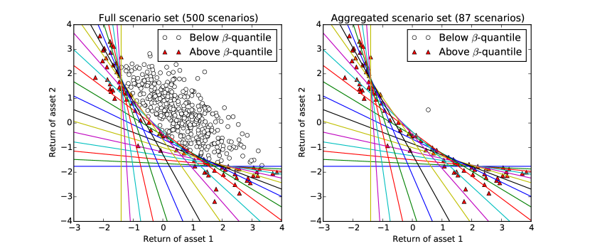
Figure 1: Return points of two assets with loss below the $\beta$-quantile for all non-negative portfolios (left) and aggregated scenario set (right)

Assuming $\mathbb{E}\left[Y|Y\in\mathcal{R}^{c}\right]\in\mathcal{R}_{Y,\mathcal{X}}^{c}$, as well as preserving the value of a tail risk measure, the aggregated random vector has the additional property of preserving the overall expected return of the original random vector. The following corollary taken from [FTW17] summarizes this result and provides sufficient conditions so that (3) holds.

Corollary 3.1.

Suppose $\mathcal{R}_{Y,\mathcal{X}}(\beta)\subseteq\mathcal{R}\subset\mathbb{R}^{d}$, $Y$ is a continuous random vector with support $\mathcal{Y}=\mathbb{R}^{d}$, and $\mathcal{X}$ contains at least two linearly independent elements. Then $Y$ satisfies (3). In addition, if $\mathcal{R}^{c}$ is convex then $\tilde{Y}=\psi_{\mathcal{R}}(Y)$ satisfies condition (4) and so for all $x\in\mathcal{X}$ we have:

$$\rho_{\beta}\left(-x^{T}Y\right) =\rho_{\beta}\left(-x^{T}\tilde{Y}\right),$$

$$\mathbb{E}\left[x^{T}Y\right] =\mathbb{E}\left[x^{T}\tilde{Y}\right].$$

In Section 2.2 we showed that under mild conditions when using an approximate risk region, a misspecification for a particular decision will decrease the value of the $\beta\operatorname{-VaR}$ and $\beta\operatorname{-CVaR}$. Building on this result, the following corollary gives a condition under which the optimal solution yielded by using an approximate risk region is also optimal for the true problem.

Corollary 3.2.

Under assumptions (A) and (B), for the problems (P1), (P2) and (P3), suppose that replacing the solution the random vector $Y$ with the aggregated random vector $\psi_{\mathcal{R}}(Y)$ for an approximate risk region $\mathcal{R}$ yields an optimal solution $\hat{x}$. Then, if $\mathcal{R}$ is valid for $\hat{x}$ and the aggregation condition holds for $\mathcal{R}$ then $\hat{x}$ is also an optimal solution for the true problem.

Proof.

We prove this only for P1. The proofs for the other problems are very similar. First note that (5) implies that $\beta\operatorname{-CVaR}\left(-\hat{x}^{T}\psi_{\mathcal{R}}(Y))\right)=\beta\operatorname{-CVaR}\left(-\hat{x}^{T}Y)\right)$ by Proposition 2.8. Note also that since $\mathbb{E}\left[-x^{T}\psi_{\mathcal{R}}(Y)\right]=\mathbb{E}\left[-x^{T}Y\right]$ for all $x\in\mathbb{R}^{d}$ that $\hat{x}$ is feasible with respect to the true problem. Now, if $\tilde{x}$ is an optimal solution to the true problem then,

$$\beta\operatorname{-CVaR}(-\tilde{x}^{T}Y)) \geq\beta\operatorname{-CVaR}\left(-\tilde{x}^{T}\psi_{\mathcal{R}}(Y)\right)\qquad\text{by Proposition~{}\ref{prop:low-var}}$$

$$\geq\beta\operatorname{-CVaR}\left(-\hat{x}^{T}\psi_{\mathcal{R}}(Y))\right)\qquad\text{by definition of }\hat{x}$$

$$=\beta\operatorname{-CVaR}(-\hat{x}^{T}Y)).$$

Hence, $\hat{x}$ is optimal with respect to the true problem. ∎

This result guarantees a certain robustness to misspecification of the approximate risk region. Although checking whether an approximate risk region is valid for a decision could in principle be used as an optimality check, we will not use it in this way as checking directly condition (5) may be difficult. As will be seen in Section 7 we instead will rely on out-of-sample testing to verify the quality of a solution.

3.2 Risk regions for elliptical distributions

In order to exploit risk regions for scenario generation one has to be able to characterize these in a way which allows one to conveniently test whether or not a point belongs to it. In our previous paper, we were able to do this in the case where the asset returns have elliptical distributions. Elliptical distributions are a general class of distributions which include, among others, multivariate Normal and multivariate $t$-distributions. See [FKN89] for a full overview of the subject.

Definition 3.3 (Elliptical Distribution).

Let $X=(X_{1},\ldots,X_{d})$ be a random vector in $\mathbb{R}^{d}$, then $X$ is said to be spherical, if

$$X\sim UX\qquad\text{for all orthonormal matrices }U$$

where $\sim$ means the two operands have the same distribution function.

Let $Y$ be a random vector in $\mathbb{R}^{d}$, then $Y$ is said to be elliptical if it can be written $Y=P^{T}X+\mu$ where $P\in\mathbb{R}^{d\times d}$ is non-singular, $\mu\in\mathbb{R}^{d}$, and $X$ is random vector with spherical distribution. Such an elliptical distribution will be denoted $\operatorname{Elliptical}\left(X,\mu,P\right)$.

This definition says that a random vector with a spherical distribution is rotation invariant, and that an elliptical distribution is an affine transformation of a spherical distribution. Elliptical distributions are convenient in the context of portfolio selection as we can write down exactly the distribution of loss of a portfolio. In particular, if $Y\sim\operatorname{Elliptical}\left(X,\mu,P\right)$ and $x\in\mathbb{R}^{d}$ then

$$-x^{T}Y\sim\left\|\kern 0.50003ptPx\kern 0.50003pt\right\|X_{1}-x^{T}\mu,$$

where $\left\|\kern 0.50003pt\cdot\kern 0.50003pt\right\|$ denotes the standard Euclidean norm and $X_{1}$ is the first component of the spherical random vector $X$. Therefore, the $\beta$-quantile of the loss $-x^{T}Y$ is as follows:

$$F_{x}^{-1}(\beta)=\left\|\kern 0.50003ptPx\kern 0.50003pt\right\|F^{-1}_{X_{1}}\left(\beta\right)-x^{T}\mu.$$

For $Y\sim\operatorname{Elliptical}\left(X,\mu,P\right)$, we can thus rewrite the risk region in (1) as follows:

$$\mathcal{R}_{Y,\mathcal{X}}(\beta):=\bigcup_{x\in\mathcal{X}}\{y\in\mathbb{R}^{d}:-x^{T}y\geq\left\|\kern 0.50003ptPx\kern 0.50003pt\right\|F^{-1}_{X_{1}}\left(\beta\right)-x^{T}\mu\}.$$ (6)

In this form it is still difficult to check whether a given point $\tilde{y}\in\mathbb{R}^{d}$ belongs to it. In [FTW17] we provided a more convenient characterization of the risk region for elliptical returns. This characterization makes use of the conic hull of the feasible region $\mathcal{X}\subset\mathbb{R}^{d}$.

Definition 3.4 (Convex cones and conic hull).

A set $K\subset\mathbb{R}^{d}$ is a cone if for all $x\in K$ and $\lambda\geq 0$ we have $\lambda x\in K$. A cone is convex if for all $x_{1},x_{2}\in K$ and $\lambda_{1},\lambda_{2}\geq 0$ we have $\lambda_{1}x_{1}+\lambda_{2}x_{2}\in K$. The conic hull of a set $\mathcal{A}\subset\mathbb{R}^{d}$ is the smallest convex cone containing $\mathcal{A}$, and is denoted $\operatorname{conic}\left(\mathcal{A}\right)$.

For example, suppose that our feasible region consists of portfolios with non-negative investments (i.e. no short-selling) and whose total investment is normalized to one, that is:

$$\mathcal{X}=\{x\in\mathbb{R}^{d}:\sum_{i=1}^{d}x_{i}=1,\ \ x_{i}\geq 0\text{ for each }i=1,\ldots,d\},$$

then the conic hull of this is the positive quadrant, that is $\operatorname{conic}\left(\mathcal{X}\right)=\mathbb{R}^{d}_{+}$. The alternative characterization also makes use of projections.

Definition 3.5 (Projection).

Let $C\subset\mathbb{R}^{d}$ be a closed convex set, then for any point $y\in\mathbb{R}^{d}$ we define its projection onto $C$ to be the unique point $p_{C}(y)\in C$ such that

$$\inf_{x\in C}\left\|\kern 0.50003ptx-y\kern 0.50003pt\right\|=\left\|\kern 0.50003ptp_{C}(y)-y\kern 0.50003pt\right\|.$$

We are now ready to give a characterization of the risk region. For this we use the following convenient abuse of notation: for a set $\mathcal{A}\subset\mathbb{R}^{d}$ and a matrix $T\in\mathbb{R}^{d\times d}$, we write $T\left(\mathcal{A}\right):=\{Ty:y\in\mathcal{A}\}$. The following result was proved in [FTW17].

Theorem 3.6.

Suppose $Y\sim\operatorname{Elliptical}\left(X,P,\mu\right)$, $\mathcal{X}\subseteq\mathbb{R}^{d}$ is convex and let $K=\operatorname{conic}\left(\mathcal{X}\right)$. Then the risk region can be characterized exactly as follows:

$$\mathcal{R}_{Y,\mathcal{X}}(\beta)=P^{T}\left(\{\tilde{y}\in\mathbb{R}^{d}:\left\|\kern 0.50003ptp_{K^{\prime}}(\tilde{y}-\mu)\kern 0.50003pt\right\|\geq F_{X_{1}}^{-1}\left(\beta\right)\}\right),$$ (7)

where $K^{\prime}=PK$ is a linear transformation of the conic hull $K$.

When $\mu=0$ and $P=I_{d}$ the risk region can be simplified to $\mathcal{R}_{Y,\mathcal{X}}(\beta)=\left(\{\tilde{y}\in\mathbb{R}^{d}:\left\|\kern 0.50003ptp_{K}(y)\kern 0.50003pt\right\|\geq F_{X_{1}}^{-1}\left(\beta\right)\}\right)$. This allows us to interpret the projection of $y$ onto $K$ as the portfolio which leads to the largest loss.

3.3 Testing membership to a risk region

Scenario generation algorithms which exploit risk regions rely on the ability to test membership of the risk region for randomly sampled points. The characterization of the risk region for portfolio selection problems given in (7) relies on one being able to calculate the conic hull of the set of feasible portfolios, and also the ability to project points onto a transformation of this. In Section 3.3.1 we show how one can find the conic hull of the feasible region for typical constraints of a portfolio selection problem. This conic hull is a finitely generated cone. In Section 3.3.2 we show how one can project points onto this type of cone. Finally in Section 3.3.3 we briefly discuss the computational issues for the membership tests.

3.3.1 Conic hull of feasible region

In portfolio problems, the feasible region is usually defined by linear constraints, that is $\mathcal{X}=\{x\in\mathbb{R}^{d}:Ax\leq b\}$, where $A\in\mathbb{R}^{m\times d}$ and $b\in\mathbb{R}^{m}$. That is, the feasible region is the intersection of a finite number of half-spaces. It is a well-known fact that any such intersection can be written as the convex hull of a finite number of points plus the conical combination of some more points (see Theorem 1.2 in [Zie08] for example). That is, there exists $x_{1},\ldots,x_{k}\in\mathbb{R}^{d}$ and $y_{1},\ldots,y_{l}\in\mathbb{R}^{d}$ such that

$$\mathcal{X}=\{\sum_{i=1}^{k}\lambda_{i}x_{i}+\sum_{j=1}^{l}\nu_{j}y_{j}:\lambda,\nu\geq 0,\ \sum_{i=1}^{k}\lambda_{i}=1\}.$$ (8)

The conic hull of this region is the following finitely generated cone:

$$\operatorname{conic}\left(\mathcal{X}\right)=\{\sum_{i=1}^{k}\lambda_{i}x_{i}+\sum_{j=1}^{l}\nu_{j}y_{j}:\lambda,\nu\geq 0\}.$$

To express the intersection of half-spaces in the form (8), we could use Chernikova’s algorithm (also known as the double description method) [Che65, LV92]. Every finitely generated cone can also be written as a polyhedral cone, that is, of the form $\{x\in\mathbb{R}^{d}:Dx\geq 0\}$, and vice versa (see [Zie08, Chapter 1]). Chernikova’s algorithm again provides a concrete method for going between these two different representations. Although these two representations are mathematically equivalent, as we shall see, they are algorithmically different.

We will suppose the constraints for our portfolio selection problem have the following form:

$$\mathcal{X}=\left\{x\in\mathbb{R}^{d}:\begin{split}\mathbf{1}^{T}x&=c\\ a_{i}^{T}x&\leq b_{i}\qquad\text{for }i=1,\ldots,m,\\ x&\geq 0,\end{split}\right\}$$ (9)

where $\mathbf{1}$ is column vector of ones and $c>0$. The first of these constraints specifies the total of amount of capital to be invested, the inequalities represent other constraints such as quotas on the amount one can invest in a specific company or industry. In this case, we can describe immediately the conic hull as a polyhedral cone.

Proposition 3.7.

Let $\mathcal{X}$ be the set defined in (9) and let

$$\mathcal{Y}=\left\{x\in\mathbb{R}^{n}:\left(\frac{b_{i}}{c}\mathbf{1}-a_{i}\right)^{T}x\geq 0\text{ for }i=1,\ldots,m,\ x\geq 0\right\}$$

then $\operatorname{conic}\left(\mathcal{X}\right)=\mathcal{Y}$.

Proof.

Given that $\mathcal{X}$ is convex, to show that $\operatorname{conic}\left(\mathcal{X}\right)=\mathcal{Y}$, it suffices to show that

$$x\in\mathcal{Y}\setminus{\{0\}}\Longleftrightarrow\ \exists\ \lambda>0\text{ such that }\lambda x\in\mathcal{X}.$$

We demonstrate first the forward implication. Suppose $x\in\mathcal{Y}\setminus{\{0\}}$. Then, given that $x>0$, we must have $v:=\mathbf{1}^{T}x>0$. Then, setting $\lambda=\frac{c}{v}$, we have

$$\mathbf{1}^{T}(\lambda x)=v\frac{c}{v}=c.$$

Since $\mathcal{Y}$ is a cone, we have $\lambda x\in\mathcal{Y}$, hence

$$(\frac{b_{i}}{c}\mathbf{1}-a_{i})^{T}\frac{c}{v}x\ \geq\ 0$$

$$\therefore\qquad \frac{c}{v}a_{i}^{T}x\ \leq\ \frac{b_{i}}{c}\frac{c}{v}\underbrace{\mathbf{1}^{T}x}_{=v}$$

$$\therefore\qquad a_{i}^{T}(\frac{c}{v}x)\ \leq\ b_{i}$$

and so $\lambda x\in\operatorname{conic}\left(\mathcal{X}\right)$.

We now prove the backwards implication. Suppose $x\in\operatorname{conic}\left(\mathcal{X}\right)\setminus\{0\}$. Then there exists $\lambda>0$ such that $\lambda x\in\mathcal{X}$, that is

$$\mathbf{1}^{T}\lambda x =c$$

$$a_{i}^{T}\lambda x \leq b_{i}$$

Therefore,

$$\frac{a_{i}^{T}\lambda x}{\mathbf{1}^{T}\lambda x}\ \leq\ \frac{b_{i}}{c}$$

and so $$\left(\frac{b_{i}}{c}\mathbf{1}-a_{i}\right)^{T}x\ \geq\ 0.$$

Hence $x\in\mathcal{Y}$ as required. ∎

Figure 2: Conic hull from simple quota constraints given $x_{1}+x_{2}=1$ and $x_{1},x_{2}\geq 0$

Figure 2 shows how simple constraints in $\mathbb{R}^{2}$ affect the conic hull of the feasible region given the total investment and positivity constraints.

3.3.2 Projection onto a finitely generated cone

First, suppose that we can represent the conic hull of the feasible region $\mathcal{X}\subset\mathbb{R}^{d}$ as a finitely generated cone with $k$ generators, that is $K=\{Ay:y\geq 0\}$ where $A\in\mathbb{R}^{k\times d}$. By definition, the projection of a point $x_{0}\in\mathbb{R}^{d}$ can be found by solving the following quadratic program:

$$\underset{y\geq 0}{\operatorname{minimize}}\ \ \left\|\kern 0.50003ptAy-x_{0}\kern 0.50003pt\right\|_{2}^{2}$$ (10)

In particular, if $y^{*}$ is the optimal solution then $p_{K}(x_{0})=Ay^{*}$. By formulating the KKT conditions [BV04, Chapter 5] of this problem, it can be seen that this problem is equivalent to solving the following linear complementarity problem (LCP):

$$\text{Find }y,z\in\mathbb{R}^{d}\text{ such that }$$

$$z-A^{T}Ay =-A^{T}x_{0}$$

$$z^{T}y =0$$

$$y,z \geqslant 0.$$

If $(y,z)$ is a solution to the above problem, then the required projection is $p_{K}(x_{0})=Ay$. LCPs can be solved by more specialized algorithms than standard quadratic programs such as Lemke’s algorithm [CPS92].

Now, suppose instead we have a polyhedral characterization of the conic hull, that is a cone of the form:

$$K=\{x\in\mathbb{R}^{d}:Bx\geq 0\}.$$ (11)

The projection of a point $x_{0}\in\mathbb{R}^{d}$ onto the polyhedral cone in (11) is the solution of the following quadratic program:

$$\underset{x}{\operatorname{minimize}}\ \left\|\kern 0.50003ptx-x_{0}\kern 0.50003pt\right\|_{2}^{2}$$

subject to $$Bx\geq 0.$$

Although the former problem in (10) can often be solved more efficiently using specialized algorithms, we will in practice use both approaches. For conic hulls with a small number of extremal rays, for example $K=\mathbb{R}_{+}^{d}$ we will use use the former method. As we add more constraints to the problem, we have found from experience that the number of extremal rays can exponentially increase, which for the former approach leads to cumbersomely large LCP problems. In this case we will use the polyhedral representation for projection.

3.3.3 Computational issues

Given that testing membership of the risk region (for elliptically distributed returns) involves solving a small LCP or quadratic program, using this methodology could potentially become computationally expensive, especially if used to construct large scenario sets for high dimensional problems. However, this issue can be mitigated in a few ways. Firstly, the membership test for a point can be conducted independently from that of another point, which means that membership tests for a large number of points is naturally parallelizable. Secondly, for the case where the case $K\subseteq\mathbb{R}^{d}_{+}$ the loss function $y\mapsto-x^{T}y$ is monotonic. Therefore, if we have set of points $y_{1},\ldots,y_{k}$ which are in the risk region, we know that a point $\tilde{y}$ is also in the risk region if it is dominated by any of these points. A similar shortcut exists for testing if $\tilde{y}$ is in the non-risk region. Finally, the membership test could also be made more efficient, by directly testing the condition $\left\|\kern 0.50003ptp_{K}(y)\kern 0.50003pt\right\|\leq\alpha$ without calculating the full projection $p_{K}(y)$. For example, the quadratic program used to calculate the projection could be solved only to an accuracy sufficient to test this condition. This could be easily implemented through a callback function in the quadratic program solver.

4 Scenario generation

In this Section we show how risk regions can be exploited for the purposes of scenario generation. In Section 4.1 we present two specific methods which work essentially by prioritizing the construction of scenarios in the risk region. In Section 4.2 we propose a new heuristic algorithm based on the SAA method [KSHdM01]. This heuristic boosts the performance of the proposed sampling algorithm through the addition of artificial constraints to the problem.

4.1 Aggregation sampling and reduction

In [FTW17] we proposed two methods to exploit risk regions. The first of these allows the user to specify the final number of scenarios in advance. The algorithm, which is called aggregation sampling, samples scenarios, aggregating all samples in the non-risk region and keeping all in the risk region, until we have the required number of risk scenarios, that is the required number of scenarios in the risk region. This is described in Algorithm 1.

input : $\mathcal{R}\subset\mathbb{R}^{d}$ approximate risk region, $N_{\mathcal{R}}$ number of required risk scenarios

output : $\{(y_{s},p_{s})\}_{s=1}^{N_{\mathcal{R}}+1}$ scenario set

$n_{\mathcal{R}^{c}}\leftarrow 0$,  $n_{\mathcal{R}}\leftarrow 0$, $y_{\mathcal{R}^{c}}=\mathbf{0}$;

while $n_{\mathcal{R}}<N_{\mathcal{R}}$ do

       Sample new point $y$;

       if $y\in\mathcal{R}$ then

             $n_{\mathcal{R}}\leftarrow n_{\mathcal{R}}+1$; $y_{n_{\mathcal{R}}}\leftarrow y$;

            

       end if

      else

             $n_{\mathcal{R}^{c}}\leftarrow n_{\mathcal{R}^{c}}+1$; $y_{\mathcal{R}^{c}}\leftarrow\frac{1}{n_{\mathcal{R}^{c}}+1}\left(n_{\mathcal{R}^{c}}y_{\mathcal{R}^{c}}+y\right)$

       end if

      

end while

foreach $i$ in $1,\ldots,N_{\mathcal{R}}$ do $p_{i}\leftarrow\frac{1}{\left(n_{\mathcal{R}^{c}}+N_{\mathcal{R}}\right)}$;

if $n_{\mathcal{R}^{c}}>0$ then

       $p_{n_{\mathcal{R}^{c}}+1}\leftarrow\frac{n_{\mathcal{R}^{c}}}{n_{\mathcal{R}^{c}}+\mathcal{N}_{\mathcal{R}}}$;

      

end if

else

       Sample new point $y$;

       $n_{\mathcal{R}^{c}}\leftarrow 1$; $y_{N_{\mathcal{R}}+1}\leftarrow y$;

      

end if

$p_{N_{\mathcal{R}}+1}\leftarrow\frac{n_{\mathcal{R}^{c}}}{n_{\mathcal{R}^{c}}+N_{\mathcal{R}}}$

Algorithm 1 Aggregation sampling

Let $q=\mathbb{P}\left(Y\in\mathcal{R}_{Y,\mathcal{X}}^{c}\right)$ be the probability of the non-risk region, and $n$ be the number of risk scenarios required. Define $N(n)$ to be the effective sample size from aggregation sampling, that is, the number of draws until the algorithm terminates. The quantity $N(n)$ is a random variable:

$$N(n)\sim n+\mathcal{NB}(n,q),$$

where $\mathcal{NB}(N,q)$ denotes a negative binomial random variable. Recall that a negative binomial random variable $\mathcal{NB}(n,q)$ is the number of failures in a sequence of Bernoulli trials with probability of success $q$ until $n$ successes have occurred. The expected effective sample size of aggregation sampling is thus as follows:

$$\mathbb{E}\left[N(n)\right]=n+n\frac{q}{1-q}$$

The expected effective sample size can be thought of as the sample size required for basic sampling to produce the same number of scenarios in the risk region. The difference between the desired number of risk scenarios, and expected effective sample size is proportional to the ratio $\frac{q}{1-q}$. In particular, as the probability of the non-risk region approaches one, this gain tends to infinity.

The converse to aggregation sampling is sampling a set of a given size $n$ and then aggregating all scenarios in the risk region of the underlying distribution. We call this aggregation reduction. This can be viewed as a sequence of $n$ Bernoulli trials, where success and failure are defined in the same way as described above. The number of scenarios in the reduced sample, $R(n)$ is as follows:

$$R(n)\sim n-\mathcal{B}(n,q)+1$$

where $\mathcal{B}(n,q)$ denotes a binomial random variable. The expected reduction in scenarios in aggregation reduction is thus $nq-1$.

The reason why aggregation sampling and aggregation reduction work is that, for large samples, they are equivalent to sampling from the aggregated random vector. Suppose that $Y_{1},Y_{2},\ldots$ is a sequence of independently identically distributed (i.i.d.) random vectors with the same distribution as $Y$, then $\psi_{\mathcal{R}}(Y_{1}),\psi_{\mathcal{R}}(Y_{2}),\ldots$ is a sequence of i.i.d. random vectors with the same distribution as the aggregated random vector $\psi_{\mathcal{R}}(Y)$. Denote by $\tilde{\rho}_{n,\beta}(x)$ the value of the tail-risk measure for the decision $x\in\mathcal{X}$ for the sample $\psi_{\mathcal{R}}(Y_{1}),\ldots,\psi_{\mathcal{R}}(Y_{n})$, and by $\hat{\rho}_{n,\beta}$ the analogous function the scenario set constructed by aggregation sampling. The following result, adapted from [FTW17] for the portfolio selection problem, gives precise conditions under which aggregation sampling is asymptotically valid.

Theorem 4.1.

Suppose the following conditions hold:

1. For each $x\in\mathcal{X}$, $F_{x}$ is strictly increasing and continuous in some neighborhood of $F_{x}^{-1}(\beta)$

2. $\mathbb{E}\left[\ Y|Y\in\mathcal{R}^{c}\ \right]\in\operatorname{int}\left(\mathcal{R}_{\mathcal{X}}^{c}\right)$

3. $\mathcal{X}$ is compact.

Then, with probability 1, for $n$ large enough $\tilde{\rho}_{n,\beta}\equiv\hat{\rho}_{N(n),\beta}$.

See [FTW17, Section 4] for a full proof of the consistency of these algorithms.

4.2 Ghost constraints

We noted above that the performance of our methodology improves as the probability of the non-risk region increases. In particular, the expected effective sample size in aggregation sampling increases as the probability of the non-risk risk region increases. Now, by its definition (2) the non-risk region grows as the problem becomes more constrained. This suggests that it may be helpful to add constraints to our problem which shrink the set of feasible portfolios, but which are not themselves active, in the sense that their presence does not affect the set of optimal solutions. We will refer to a constraint added to a problem to boost the performance of our methodology, loosely, as a ghost constraint.

Finding non-active constraints to add to our problem is non-trivial as it relies on some knowledge of the optimal solution set. Moreover, even verifying whether or not a particular constraint is active is difficult in general for stochastic programs. For a deterministic objective function which is convex and for which all constraints are convex (and the optimal solution is unique) a constraint $\{x:g(x)\leq 0\}$ is active if and only if it is binding at the optimal solution $x^{*}$, that is $g(x^{*})=0$. For a stochastic program, we are typically solving a scenario-based approximation and so a constraint which is not binding with respect to the scenario-based approximation may be binding with respect to the true problem and vice versa. A rigorous test of whether a ghost constraint is active in the sense above is beyond the scope of this paper. We simply promote the idea here that ghost constraints may be a useful way of finding better solutions.

We resort to heuristic rules to choose ghost constraints. For example, one could constrain our set of feasible portfolios to some neighborhood of a good quality solution. This suggests an iterative procedure whereby one samples scenario sets using aggregation sampling, solves the resulting problems, adjusts the problem constraints and then resamples. In Algorithm 2 we propose such a heuristic procedure based on the sample average approximation (SAA) method of [KSHdM01]. We call this procedure the SAA method with ghost constraints. Like with the original SAA method, this algorithm is presented in a very general form, as the update rules, such as how the bounds are adjusted in each iteration, can be implemented in many different ways. In Section 7 we test this algorithm on a realistic and difficult problem.

Initialise $l_{i}=-\infty,u_{i}=\infty$ for each $i=1,\ldots,d$;

do

       Add constraints $l\leq x\leq u$ to problem;

       Construct risk region $\mathcal{R}$ for problem;

       for $i=1,\ldots,M$ do

             Generate a sample of size $N$ using aggregation sampling with risk region $\mathcal{R}$;

             Solve corresponding problem with objective value $\nu_{N}^{m}$ and optimal solution $\hat{x}_{N}^{m}$;

             Estimate optimality gap of solution and the variance of the optimality gap;

            

       end for

      Increase size of $N$;

       Adjust bounds $l$ and $u$;

      

until Optimality gap and variance are sufficiently small for some $m$;

Choose the best solution $\hat{x}$ among all candidate solutions $x_{N}^{m}$ produced, using a screening and selection procedure.

Algorithm 2 Sample average approximation method with ghost constraints

5 Probability of the non-risk region

The benefit of aggregation sampling and reduction depends on the probability of the non-risk region. As was observed in [FTW17] the probability of the non-risk region tends to decrease as the problem dimension increases, but increases as we tighten our problem constraints, and as we increase $\beta$, the level of the tail risk measure. In this section we make some empirical observations on how this probability varies with heaviness of the tails, and the correlations of the distribution.

The first observation is that in the presence of positivity constraints, the probability of the non-risk region increases as the the correlation between random variables increases. This can be seen in Figure 3 which plots the probability of the risk region as a function of correlation for some two-dimensional distributions. An intuitive explanation for this type of behavior is that in the case of positive correlations there is much more overlap in the risk regions of the individual portfolios.

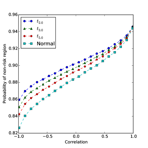
Figure 3: Correlation vs. Probability of non-risk region for some 2-dimensional elliptical distributions, positivity constraints and $\beta=0.95$

The extent to which probabilities vary with correlation seems to be much greater in higher dimensions. In Figure 4 we have plotted for Normal returns and a range of dimensions, the probabilities of the non-risk region for a particular type of correlation matrix: $\Lambda\left(\rho\right)\in\mathbb{R}^{d\times d}$ where $\Lambda(\rho)_{ij}=\rho$ for $i\neq j$ and $\rho>0$. In the case of $\rho=0$, the probability decays very quickly to zero as the dimension increases, whereas as when $\rho$ is close to one, the probability of the non-risk region approaches $\beta$ for all dimensions.

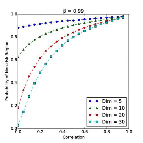
Figure 4: Probability of non-risk region for a range of correlation matrices and dimensions for Normal returns

Our next observation is that the probability of the non-risk region seems to increase as the tails of the distributions become heavier. In Figure 5 are plotted the probabilities of risk regions for some spherical distributions and a range of dimensions. Note that multivariate t-distributions have heavier tails than the multivariate Normal distribution, but the tails get lighter as the degrees of freedom parameter increases. This phenomenon can also be observed in Figure 3.

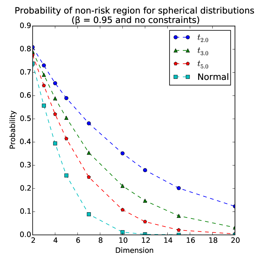
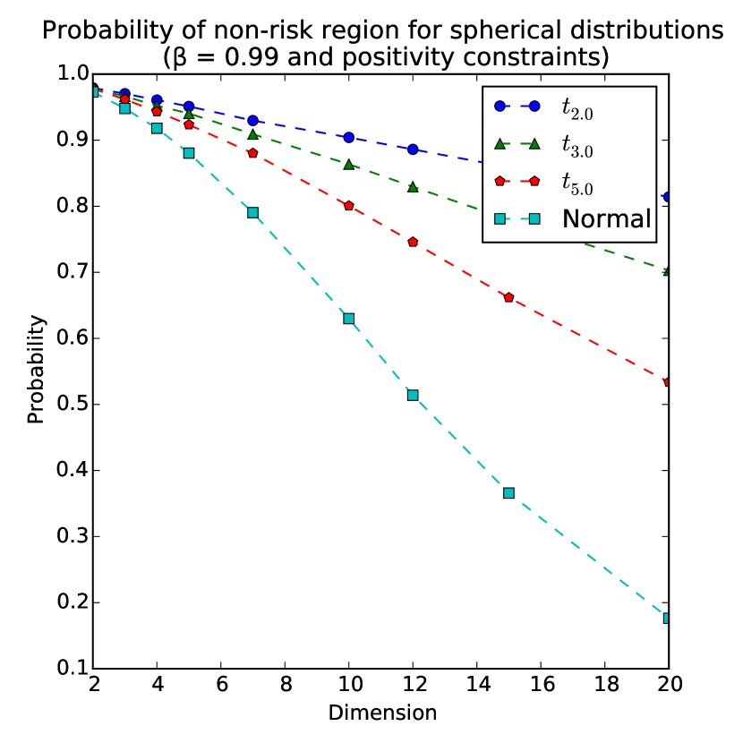
Figure 5: Probability of non-risk regions for different spherical distributions and dimensions

The observations made in this section suggest that that the application of our methodology will be particularly effective when applied to real stock data tend to be positively correlated and have heavy tails.

6 Numerical tests

In this Section we test the numerical performance of our methodology for realistic distributions. There are three parts to these tests: the calculation of the probability of the non-risk region for a range of distributions and constraints, the performance of aggregation sampling, and the performance of aggregation reduction. To allow us to measure the quality of the solutions yielded by the proposed methods, the majority of the tests are performed for elliptical distributions on problems without integer variables. These problems can be solved exactly using other methods. In Section 6.1 we describe our experimental set-up, in particular we justify the distributions constructed for these experiments. The remaining three sections detail the individual experiments and their results.

6.1 Experimental set-up

For robustness we will use several randomly constructed distributions for each family of distribution and each dimension we are testing. We construct these by fitting parametric distributions to real data. We use real data rather than arbitrarily generated problem parameters for two reasons. Firstly, generating parameters which correspond to well-defined distributions can be problematic. For example, for the moment matching algorithm, there may not exist a distribution which has a given set of target moments (see [KME00] and [JR51] for instance). Secondly, as was observed in Section 5, the probability of the non-risk region can vary widely, and so it is most meaningful to test the performance of our methodology for distributions which are realistic for portfolio selection problems.

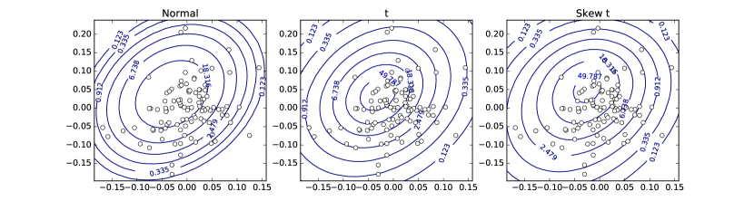
Figure 6: Contour plots of distributions fitted to financial return data for two assets

We construct our distributions from monthly return data from between January 2007 and February 2015 for 90 companies in the FTSE 100 index. For each dimension in the test, we randomly sample five sets of companies of that size, and for each of these sets fit Normal, t distributions and Skew-t distributions to the associated return data. Figure 6 shows for two stocks the contours of the fitted density functions overlaying the historical return data. For the $t$ distributions we fix the degrees of freedom parameter to $4.0$. This is so that we can more easily compare the effect of heavier tails on the results of our tests. We allow the corresponding parameter for the skew-t distributions to be fitted from the data.

These three distributions are fitted to the data through maximum likelihood estimation, weighing each observation equally; our aim here is not to construct distributions which accurately capture the uncertainty of future returns, but to simply construct distributions which are realistic for this type of problem. We also use scenario sets constructed using the moment-matching algorithm. For each random set of companies, we calculate all the required marginal moments and correlations from their historical returns, and use these as input to the moment-matching algorithm. To allow us to compare results, the same constructed distributions are used across the three sets of numerical tests.

Throughout this section we use the $\beta\operatorname{-CVaR}$ as our tail risk measure. This is not only because the $\beta\operatorname{-CVaR}$ leads to tractable scenario-based optimization problems, but also for elliptically distributed returns we can evaluate the $\beta\operatorname{-CVaR}$ exactly which provides us with a means to evaluate the true performance of the solutions yielded by the approximate scenario-based problems. In addition, to ensure that the non-risk region does not have negligible probability, we will assume that we always have positivity constraints on our investments (i.e. no short selling).

The first class of non-elliptical distributions we use in this paper are known as multivariate Skew-t distributions [AC03]. This class of distributions generalizes the elliptical multivariate t-distributions through the inclusion of an extra set of parameters which regulate the skewness. In this case we approximate the risk region with the risk region of the corresponding t-distribution.

The second class we use are discrete distributions constructed using the moment matching algorithm of [HKW03]. These distributions have been applied previously to financial problems [KWVZ07]. This algorithm constructs scenario sets with a specified correlation matrix and whose marginals have specified first four moments. This algorithm works by first taking a sample from a multivariate Normal distribution, and then iteratively applying transformations to this until the difference between its marginal moments and correlation matrix are sufficiently close to their target values. Since the algorithm is initialized with a sample from an elliptical distribution, the final distribution is near elliptical and we approximate the risk region for these distributions with the risk region of a multivariate normal distribution with the same mean and covariance structure.

6.2 Probability of non-risk region with quota constraints

We first estimate the probability of the non-risk region for a range of distributions, dimensions and constraints. We calculate these probabilities only for the Normal and t distributions as skew-t distributions and moment matching scenario sets use surrogate risk regions based on these distributions. The main purpose of this is to provide intuition about under what circumstances the methodology is effective: there is little to be gained from aggregating scenarios in a non-risk region of negligible probability.

For each distribution we sample 2000 scenarios and calculate the proportion of points in the non-risk region for different levels of $\beta$ and constraints. In particular, for each dimension we calculate for $\beta=0.95$, and $\beta=0.99$, and for a range of quotas. The feasible region corresponding to quota $0<q<1$ is $\{x\in\mathbb{R}^{d}:0\leq x_{i}\leq q\text{ for }i=1,\ldots,d,\ \sum_{i=1}^{d}x_{i}=1\}$. Quotas are quite a natural constraint to use in the portfolio selection problem as they ensure that a portfolio is not overexposed to one asset. The quotas may also be viewed as ghost constraints to be used in cases where the probability of the non-risk region with only positivity constraints is too small.

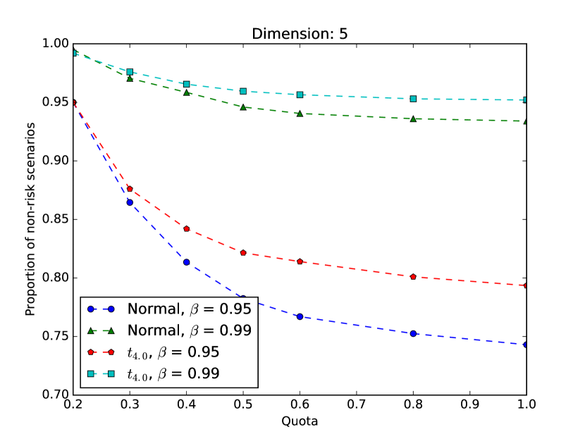
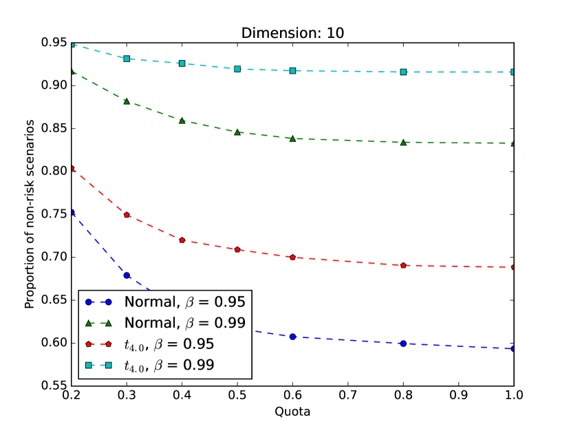
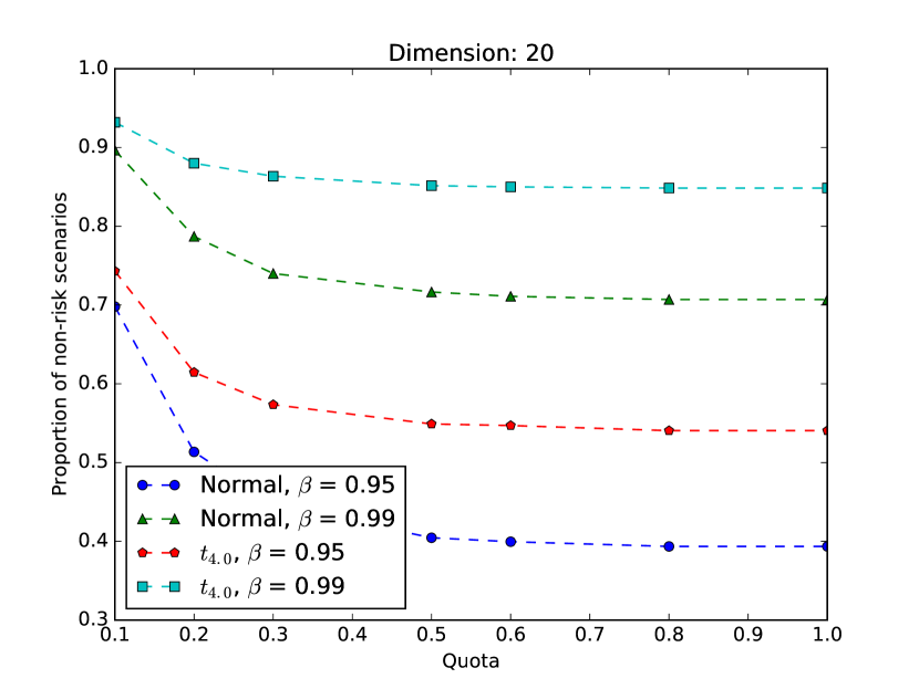
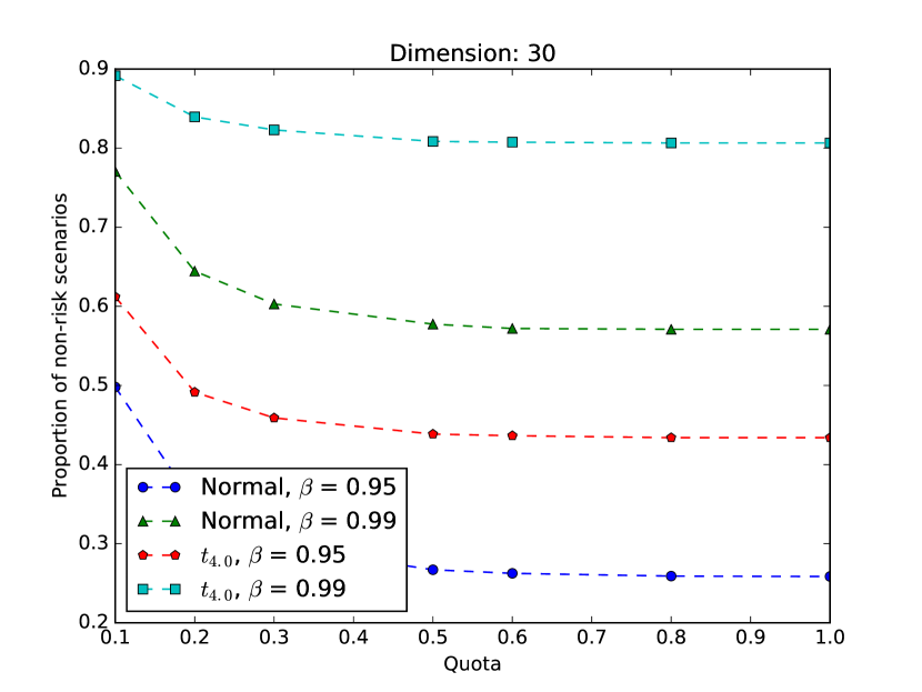
Figure 7: Proportions of non-risk scenarios

In Figure 7 for each each dimension we have tested we have plotted the results of one trial. The full results can be found in Appendix A. The first important observation from these is that the proportion of scenarios in the non-risk region, as compared to the uncorrelated case in Figure 4, is surprisingly high; even for $\beta=0.95$ and dimension 30, this proportion is non-negligible. As expected, the proportion of scenarios in the non-risk region increases as we tighten our quota. However, for higher dimensions the quotas need to be a lot tighter to make a significant difference. The plots also provide further evidence that the t distribution has non-risk regions with higher probabilities than the lighter-tailed Normal distribution. In Figure 7, the non-risk region for the $t$-distributions has probability around 0.05 to 0.1 higher for dimensions 5 and 10, and around 0.1 to 0.2 higher for dimensions 20 and 30.

6.3 Aggregation sampling

In this section we compare the quality of solutions yielded by sampling and aggregation sampling by observing the optimality gaps of the solutions that these scenario generation methods yield. For this, we use the following version of the portfolio selection problem.

$$\underset{x\geq 0}{\operatorname{minimize}}\ \beta\operatorname{-CVaR}\left(-x^{T}Y\right)$$

such that $$\ x^{T}\mu\geq\tau,$$

$$\sum_{i=1}^{d}x_{i}=1,$$

$$0\leq x\leq u,$$

where $\mu$ is the mean of the input distribution (rather than scenario set), $\tau$ is the target return and $u$ is a vector of asset quotas. The primary reason for using this formulation over those in (P2) and (P3) is that given a distribution of asset returns it is easy to select an appropriate expected target return $\tau$. For simplicity, in our tests we set $\tau=\frac{1}{n}\sum_{i=1}^{n}\mu_{i}$ which ensures that the constraint is feasible but not trivially satisfied. Notice that in the above formulation we use the deterministic constraint, $x^{T}\mu\geq\tau$ rather than $\mathbb{E}\left[x^{T}Y\right]\geq\tau$. This is because the latter constraint depends on the scenario set. Therefore, the solution from a scenario-based approximation might be infeasible with respect to the original problem, which makes measuring solution quality problematic.

In this experiment, we test the performance of the aggregation sampling algorithm for three families of distributions: the Normal distribution, the t-distribution and the skew-t distribution.

For each distribution and problem dimension we run five trials using our constructed distributions (as described in Section 6.1). Each trial consists of generating 50 scenario sets via sampling and aggregation sampling, solving the corresponding scenario-based problem for each of these sets, and calculating the optimality gap for each solution which is yielded. For each scenario generation method we then calculate the mean and standard deviation (S.D.) of the optimality gap. For the skew-t distributions, although we are able to evaluate the objective function value for any candidate solution, to find the true optimal solution value (or one close to it), we resort to solving the problem for a very large sampled set of size 200000.

The full results for this experiment can be found in Appendix B. In Figure 8 we have plotted for one trial the raw results for dimensions 10 and 30. We observe that there is a consistent improvement in solution quality in using aggregation sampling over basic sampling. In addition the solution values are much more stable. The improvement in solution quality and stability is particularly big for the $t$-distributions. This is because the probability of the non-risk region is greater for heavier-tailed distributions as observed in Section 5. Aggregation sampling even lead to consistently better solutions for the skew-t distributions where we are approximating the risk region with a risk region for a t-distribution.

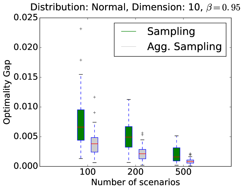
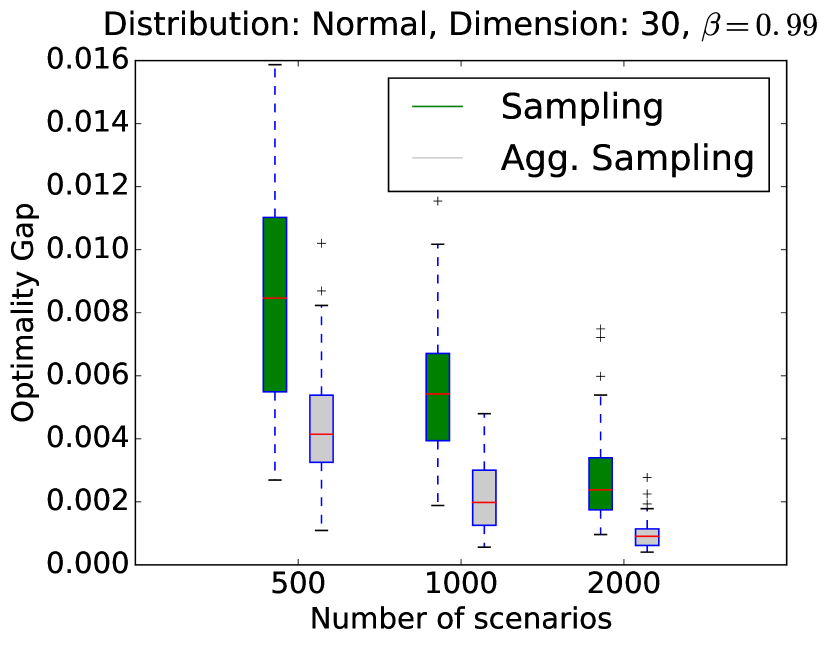
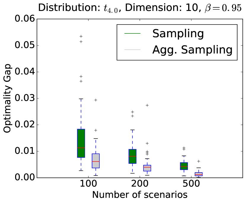
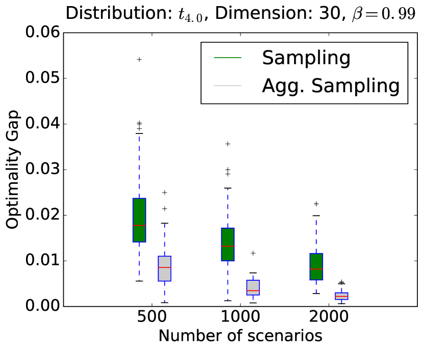
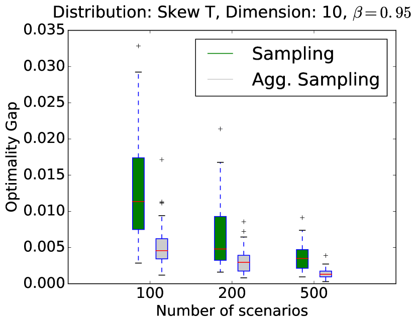
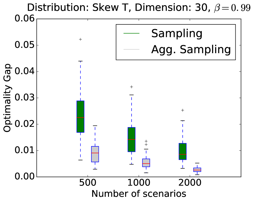
Figure 8: Stability test comparing performance of sampling and aggregation sampling

6.4 Aggregation reduction

The aim of these tests is to quantify the error induced through the use of aggregation reduction. In particular, we calculate the error induced in the optimal solution value. For a given scenario set, we aggregate the non-risk scenarios, solve the problem with respect to this reduced set, and calculate the optimality gap of this solution with respect to the original scenario set.

For these tests we use the same problem as in Section 6.3 and run tests for Normal, t and moment matching distributions. As explained in Section 4, we use the risk region of a Normal distribution to approximate the risk region for moment-matched scenario sets. For each family of distributions and problem dimension we again run five trials for different instances of the distribution. In each trial for different initial scenario set sizes, $n=100,\ 200,\ 500$, and two different levels of tail risk measure $\beta=0.95,\ 0.99$, we calculate the reduction error for 30 different scenario sets and report the mean error.

The full results can be found in Appendix C. These show that the reduction error is generally very small, in fact for almost all problems using $\beta=0.95$, there is no error induced. For $\beta=0.99$, and the smallest scenario set size $n=100$, there is a small amount of error ($<0.01$) for the Normal distributions, slightly larger errors for the heavier-tailed $t$ distribution ($<0.02$), and the largest errors (0.1-0.5) occur for reduced moment-matching scenario sets whose risk regions have been approximated with that of a Normal distribution. However, as the scenario set size is increased, all errors are reduced, and for the largest scenario set size $n=500$, there is no error induced for almost all problems.

Comparing the reduction errors with the corresponding non-risk region probabilities in Appendix A, we see that the larger errors generally occur for the higher dimensional distributions whose non-risk region has a larger probability. This is to be expected as the larger the non-risk region the more scenarios that are aggregated. In Table 33 in Appendix C we have also included the proportions of reduced scenarios for moment matching scenario sets for which we approximated the risk region with that of a Normal distribution. The proportions of reduced scenarios in this case are generally slightly higher than that of the corresponding Normal distributions. This might suggest that the surrogates for the risk region are slightly too small, but this could equally be explained by the fact that moment matching scenario sets generally have heavier tails than the corresponding Normal distribution, which, as we observed in Section 5, also leads to non-risk regions of higher probabilities. In either case, the larger errors which are induced by reducing small moment-matching scenario sets could be explained by these increased probabilities.

7 Case study

In this section we demonstrate the application of the presented methodology on a difficult problem which may occur in practice. The problem is characterized by a high-dimension, a heavy-tailed non-elliptical distribution of asset returns, and the presence of integer variables. We compare the performance of the SAA method with ghost constraints algorithm proposed in Section 4.2 against the standard SAA method using basic sampling and aggregation sampling without ghost constraints.

7.1 Problem construction

The following problem is used:

$$\underset{x,z}{\operatorname{minimize}}\ \beta\operatorname{-CVaR}\left(-x^{T}Y\right)$$

such that $$\ x^{T}\mu\geq\tau,$$

$$x_{i}\leq z_{i}\ \text{for each }i=1,\ldots,d,$$

$$\sum_{i=1}^{d}x_{i}=1,$$

$$\sum_{i=1}^{d}z_{i}=l,$$

$$0\leq x\leq u,$$

$$z_{i}\in\{0,1\}\ \text{for each }i=1,\ldots,d.$$

This problem is similar to that used in Section 6.3 except that we now use binary decision variables to limit the number of assets in which one can invest. The extra constraints involving integer variables may change the conic hull of feasible portfolios, however, the method presented in Section 3.3.1 for calculating conic hulls of feasible regions cannot handle these. We therefore ignore these constraints when constructing a risk region. This is acceptable as the resulting conic hull will contain the true conic hull. The problem is solved for $\beta=0.99$, $d=50$ assets, and maximum number of assets $l=10$. The random vector $Y$ of asset returns is constructed by fitting Skew-t distributions to historical monthly return data for companies from the FTSE100 stock index. The risk region used for this distribution is constructed as described at the end of Section 6.1.

7.2 Details of the SAA method

Estimation of optimality gap

In each iteration of the SAA method the optimality gap for each of the found solutions is calculated using the procedure described in [KSHdM01]. Let $N$ be the scenario set size and $M$ be the number of replications used in each iteration. For $m=1,\ldots,M$ denote by $g_{N}^{m}$ and $\nu_{N}^{m}$ respectively the objective function and optimal solution value corresponding to the $m$-th constructed scenario set. In this case, $g_{N}^{m}(x)=\beta\operatorname{-CVaR}(-x^{T}Y^{m})$ where $Y^{m}$ denotes the discrete random vector corresponding to the $m$-th constructed scenario set.

Estimators for the optimal solution value and objective function are given by:

$$\bar{\nu}_{N}^{M}=\sum_{m=1}^{M}\nu_{N}^{m},\qquad\bar{g}_{N}^{M}(x)=\sum_{m=1}^{M}g_{N}^{M}(x),$$

Now, an $\alpha$-level confidence interval for the optimality gap estimator by the solution $x$ is given by

$$\bar{g}_{N}^{M}(x)-\bar{\nu}_{N}^{M}+\Phi^{-1}(1-\alpha)\frac{\bar{S}_{M}^{2}}{\sqrt{M}}.$$

where $\bar{S}_{M}^{2}$ is the standard deviation of $g_{N}^{m}(x)-\nu_{N}^{m}$ over $m=1,\ldots,M$, and $\Phi$ is the cumulative distribution function for a standard Normal distribution. Note that other procedures for estimating the optimality gap exist which only require the solution of one or two problems [BM06], [SB13].

Sample sizes, replications and bounds

For this experiment, the initial sample size used to solve this problem is $N=N_{0}=200$ and at each iteration this is increased by $N_{0}/2=100$. The number of replications used in each iteration is fixed at $M=10$. These update rules have been chosen for simplicity; more sophisticated rules for updating the sample sizes and number of replications can be found in, for example, [RS13].

For the ghost constraints, the following heuristic rule is used. First denote by $\hat{x}^{m}_{N}$ for $m=1,\ldots,M$ the solutions found for each replication. At the end of each iteration the bounds $l\leq x\leq u$ are updated as follows:

$$l =\max\left(\bar{x}_{N}^{M}-\Phi^{-1}(\alpha)\frac{\bar{\sigma}^{M}_{N}}{\sqrt{M}},0\right),$$

$$u =\min\left(\bar{x}_{N}^{M}+\Phi^{-1}(\alpha)\frac{\bar{\sigma}^{M}_{N}}{\sqrt{M}},1\right),$$

where $\bar{x}_{N}^{M}$ and $\bar{\sigma}_{N}^{M}$ are the element-wise mean and standard deviation of the solutions $\hat{x}_{N}^{m}$ over $m=1,\ldots,M$, and the parameter $0<\alpha<1$ controls how aggressively the ghost constraints are tightened. In this experiment we use $\alpha=0.99$.

Solution validation

Given the potential dangers in approximating the risk region, and misspecifying ghost constraints, it is important to verify the quality of a solution by the calculation of its corresponding out-of-sample value [KW07]. That is, after we calculate the $\beta$-CVaR for all candidate solutions with respect to a large independently sampled scenario set for all solutions yielded by the final iteration of the SAA methods. For this experiment a sample size of 100000 is used for validation.

7.3 Results

The results to this experiment are shown in Figure 9. In Figure 9(a) is shown the best optimality gap found at the end of each iteration of the SAA method, in Figure 9(b) are shown box plots with the out-of-sample values of the final solutions yielded by each method, and to aid our interpretation of the results. In Figure 9(c) we have plotted the evolution of the probability of the non-risk region used in the SAA method with ghost constraints.

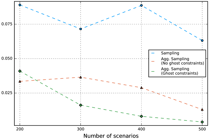
(a) Best optimality gap

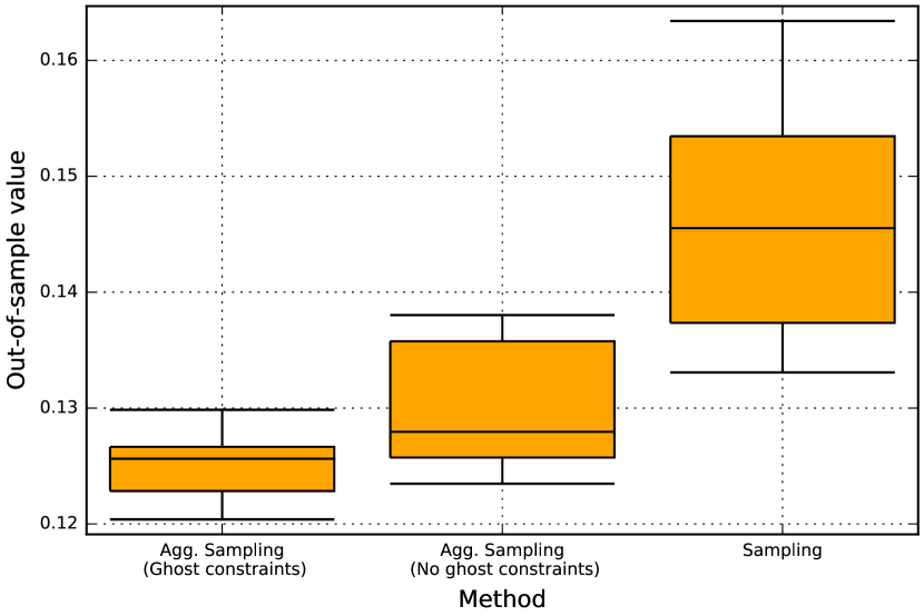
(b) Out-of-sample values

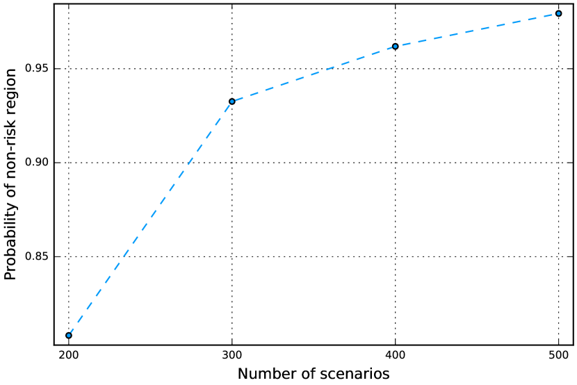
(c) Prob. of non-risk region

Figure 9: Case study results

In terms of the optimality gap and the final out-of-sample values, both aggregation sampling methods signifiantly outperform basic sampling. For the smallest sample size $N=200$, the best optimality gap of aggregation sampling with and without ghost constraints is similar, since at this point no ghost constraints have been added. As the sample size increases, the ghost constraints become tighter and the probability of the non-risk region increases. This leads to a much smaller best optimality gap for aggregation sampling with ghost constraints. Since we cannot verify that the ghost constraints added are valid, we must view this gap with some caution. However, the out-of-sample validation after the final iteration reveals that aggregation sampling with ghost constraints is indeed producing higher quality solutions than aggregation sampling without ghost constraints.

8 Conclusions

In the paper [FTW17] we proposed a general approach to scenario generation using risk regions for stochastic programs with tail risk measure. As proof-of-concept we demonstrated how this applied for portfolio selection problems for elliptically distributed returns. In this work, we have presented how this methodology may be used for more realistic portfolio selection problems, in particular those which are high-dimensional, have non-elliptical assets returns and integer decision variables.

The main issue in applying the methodology to more realistic problems was its extension to non-elliptical distributions. In order to do this, we proposed the use of approximate risk regions, and derived results which indicated our approach would be robust against small misspecifications of risk region. Although this paper was focused on portfolio selection, the results were derived for general stochastic programs, which means that using approximate risk regions could work for other problems with tail risk measures.

We tested the performance of our methodology for solving realistic problems where the return distributions were fitted from real financial return data. Aggregation sampling generally outperformed basic sampling in terms of solution quality and stability. We also showed that aggregation reduction induces almost no error in the solution for reasonably sized scenario sets. These results not only held for elliptical distributions, but also non-elliptical distributions for which we used approximate risk regions.

The effectiveness of using risk regions for scenario generation depends upon the probability of the risk region: the greater the probability of the non-risk region, the more scenarios that can be aggregated. It follows directly from the definition of risk regions that this probability decreases as the problem becomes more constrained. Based on this observation, a heuristic based on the SAA method was proposed, which adds artificial constraints, called ghost constraints, to the problem. As the algorithm progresses, the ghost constraints are tightened which in effect allows one to focus in on high quality solutions. This algorithm was demonstrated on a difficult case study problem, and was shown to significantly outperform basic sampling and aggregation sampling without ghost constraints. This algorithm was presented in a non-problem specific way and could potentially be applied to other stochastic programs with tail risk measure.

Appendix A Reduction proportion tables

The following tables list the estimated probabilities of the non-risk region for a variety of distributions constructed from real data. See Section 6.2 for details. Each table corresponds to a family of distributions at a given dimension, and each row gives the proportions for a given set of companies. In addition, the distributions corresponding the i-th row of each table of dimension $d$ have been fitted using the same set of companies.

$\beta=0.95$							$\beta=0.99$
$x\leq 1.0$	$x\leq 0.8$	$x\leq 0.6$	$x\leq 0.5$	$x\leq 0.4$	$x\leq 0.3$	$x\leq 0.2$	$x\leq 1.0$	$x\leq 0.8$	$x\leq 0.6$	$x\leq 0.5$	$x\leq 0.4$	$x\leq 0.3$	$x\leq 0.2$
0.743	0.752	0.767	0.782	0.814	0.865	0.950	0.934	0.936	0.941	0.946	0.959	0.971	0.995
0.738	0.744	0.760	0.777	0.809	0.855	0.949	0.922	0.925	0.928	0.934	0.949	0.965	0.992
0.767	0.775	0.793	0.807	0.832	0.872	0.948	0.930	0.932	0.937	0.943	0.953	0.969	0.990
0.763	0.771	0.784	0.801	0.830	0.880	0.951	0.931	0.934	0.944	0.949	0.957	0.973	0.987
0.755	0.763	0.777	0.798	0.829	0.883	0.955	0.927	0.929	0.935	0.940	0.951	0.966	0.991

Table 1: Proportion of reduced scenarios for Normal distributed returns and $d=5$

$\beta=0.95$							$\beta=0.99$
$x\leq 1.0$	$x\leq 0.8$	$x\leq 0.6$	$x\leq 0.5$	$x\leq 0.4$	$x\leq 0.3$	$x\leq 0.2$	$x\leq 1.0$	$x\leq 0.8$	$x\leq 0.6$	$x\leq 0.5$	$x\leq 0.4$	$x\leq 0.3$	$x\leq 0.2$
0.594	0.600	0.608	0.617	0.637	0.679	0.752	0.833	0.834	0.839	0.846	0.860	0.882	0.917
0.617	0.621	0.632	0.647	0.669	0.703	0.777	0.851	0.852	0.856	0.860	0.868	0.879	0.914
0.506	0.509	0.523	0.534	0.560	0.606	0.689	0.779	0.780	0.787	0.791	0.806	0.837	0.889
0.564	0.566	0.573	0.590	0.615	0.658	0.748	0.827	0.828	0.835	0.846	0.857	0.877	0.921
0.537	0.540	0.552	0.566	0.586	0.624	0.727	0.820	0.822	0.825	0.832	0.843	0.870	0.912

Table 2: Proportion of reduced scenarios for Normal distributed returns and $d=10$

$\beta=0.95$							$\beta=0.99$
$x\leq 1.0$	$x\leq 0.8$	$x\leq 0.6$	$x\leq 0.5$	$x\leq 0.3$	$x\leq 0.2$	$x\leq 0.1$	$x\leq 1.0$	$x\leq 0.8$	$x\leq 0.6$	$x\leq 0.5$	$x\leq 0.3$	$x\leq 0.2$	$x\leq 0.1$
0.394	0.394	0.400	0.405	0.447	0.513	0.698	0.707	0.707	0.711	0.717	0.740	0.787	0.896
0.325	0.326	0.332	0.342	0.392	0.457	0.635	0.653	0.653	0.655	0.662	0.696	0.740	0.851
0.344	0.344	0.348	0.354	0.389	0.460	0.668	0.648	0.648	0.653	0.656	0.683	0.743	0.870
0.384	0.385	0.390	0.401	0.440	0.507	0.708	0.695	0.695	0.698	0.704	0.740	0.782	0.896
0.417	0.418	0.424	0.432	0.479	0.540	0.738	0.727	0.727	0.730	0.735	0.764	0.813	0.906

Table 3: Proportion of reduced scenarios for Normal distributed returns and $d=20$

$\beta=0.95$							$\beta=0.99$
$x\leq 1.0$	$x\leq 0.8$	$x\leq 0.6$	$x\leq 0.5$	$x\leq 0.3$	$x\leq 0.2$	$x\leq 0.1$	$x\leq 1.0$	$x\leq 0.8$	$x\leq 0.6$	$x\leq 0.5$	$x\leq 0.3$	$x\leq 0.2$	$x\leq 0.1$
0.259	0.259	0.263	0.267	0.297	0.350	0.498	0.571	0.571	0.572	0.578	0.603	0.644	0.770
0.264	0.266	0.269	0.272	0.299	0.347	0.511	0.587	0.587	0.589	0.591	0.616	0.661	0.790
0.282	0.282	0.286	0.291	0.321	0.378	0.533	0.599	0.599	0.602	0.607	0.631	0.681	0.785
0.247	0.247	0.251	0.257	0.281	0.333	0.502	0.555	0.555	0.556	0.558	0.586	0.630	0.769
0.293	0.293	0.296	0.301	0.324	0.374	0.548	0.583	0.583	0.584	0.587	0.613	0.665	0.802

Table 4: Proportion of reduced scenarios for Normal distributed returns and $d=30$

$\beta=0.95$							$\beta=0.99$
$x\leq 1.0$	$x\leq 0.8$	$x\leq 0.6$	$x\leq 0.5$	$x\leq 0.4$	$x\leq 0.3$	$x\leq 0.2$	$x\leq 1.0$	$x\leq 0.8$	$x\leq 0.6$	$x\leq 0.5$	$x\leq 0.4$	$x\leq 0.3$	$x\leq 0.2$
0.793	0.801	0.814	0.822	0.842	0.876	0.950	0.952	0.953	0.957	0.960	0.966	0.976	0.992
0.775	0.782	0.796	0.812	0.837	0.877	0.946	0.949	0.950	0.954	0.956	0.961	0.972	0.988
0.808	0.815	0.829	0.841	0.859	0.898	0.953	0.958	0.960	0.962	0.964	0.969	0.980	0.992
0.799	0.808	0.819	0.828	0.855	0.882	0.950	0.949	0.951	0.954	0.957	0.965	0.977	0.990
0.793	0.799	0.809	0.822	0.848	0.887	0.951	0.960	0.960	0.963	0.965	0.969	0.976	0.991

Table 5: Proportion of reduced scenarios for $t_{4.0}$ distributed returns and $d=5$

$\beta=0.95$							$\beta=0.99$
$x\leq 1.0$	$x\leq 0.8$	$x\leq 0.6$	$x\leq 0.5$	$x\leq 0.4$	$x\leq 0.3$	$x\leq 0.2$	$x\leq 1.0$	$x\leq 0.8$	$x\leq 0.6$	$x\leq 0.5$	$x\leq 0.4$	$x\leq 0.3$	$x\leq 0.2$
0.689	0.691	0.700	0.709	0.720	0.750	0.804	0.916	0.916	0.917	0.919	0.926	0.931	0.949
0.711	0.713	0.719	0.730	0.742	0.769	0.829	0.923	0.924	0.925	0.926	0.930	0.940	0.956
0.616	0.617	0.630	0.640	0.656	0.677	0.754	0.895	0.896	0.898	0.900	0.905	0.915	0.935
0.642	0.642	0.647	0.657	0.672	0.703	0.783	0.896	0.896	0.900	0.904	0.913	0.925	0.941
0.652	0.655	0.666	0.675	0.690	0.723	0.785	0.905	0.905	0.907	0.908	0.913	0.924	0.944

Table 6: Proportion of reduced scenarios for $t_{4.0}$ distributed returns and $d=10$

$\beta=0.95$							$\beta=0.99$
$x\leq 1.0$	$x\leq 0.8$	$x\leq 0.6$	$x\leq 0.5$	$x\leq 0.3$	$x\leq 0.2$	$x\leq 0.1$	$x\leq 1.0$	$x\leq 0.8$	$x\leq 0.6$	$x\leq 0.5$	$x\leq 0.3$	$x\leq 0.2$	$x\leq 0.1$
0.540	0.540	0.547	0.549	0.574	0.615	0.743	0.849	0.849	0.850	0.852	0.864	0.880	0.932
0.461	0.463	0.467	0.475	0.509	0.560	0.703	0.835	0.836	0.840	0.844	0.858	0.870	0.919
0.506	0.507	0.510	0.515	0.551	0.595	0.753	0.839	0.839	0.839	0.840	0.855	0.874	0.931
0.511	0.511	0.514	0.519	0.562	0.612	0.753	0.860	0.860	0.862	0.865	0.876	0.894	0.939
0.567	0.568	0.572	0.576	0.609	0.657	0.797	0.866	0.867	0.867	0.870	0.881	0.901	0.952

Table 7: Proportion of reduced scenarios for $t_{4.0}$ distributed returns and $d=20$

$\beta=0.95$							$\beta=0.99$
$x\leq 1.0$	$x\leq 0.8$	$x\leq 0.6$	$x\leq 0.5$	$x\leq 0.3$	$x\leq 0.2$	$x\leq 0.1$	$x\leq 1.0$	$x\leq 0.8$	$x\leq 0.6$	$x\leq 0.5$	$x\leq 0.3$	$x\leq 0.2$	$x\leq 0.1$
0.434	0.434	0.436	0.439	0.459	0.491	0.612	0.806	0.806	0.807	0.808	0.823	0.840	0.891
0.466	0.466	0.468	0.469	0.495	0.532	0.649	0.821	0.821	0.823	0.824	0.838	0.853	0.897
0.443	0.443	0.445	0.448	0.474	0.512	0.637	0.821	0.822	0.822	0.824	0.834	0.854	0.898
0.444	0.445	0.448	0.454	0.470	0.513	0.635	0.812	0.813	0.814	0.814	0.823	0.841	0.889
0.417	0.417	0.419	0.421	0.444	0.487	0.617	0.808	0.808	0.810	0.811	0.823	0.844	0.891

Table 8: Proportion of reduced scenarios for $t_{4.0}$ distributed returns and $d=30$

Appendix B Aggregation sampling tables

The following tables list the relative reduction in the mean and standard deviation of optimality gaps for aggregation sampling compared with sampling for a variety of distributions. See Section 6.3 for more details.

n = 100		n = 200		n = 500
Mean Imp.	S.D. Imp.	Mean Imp.	S.D. Imp.	Mean Imp.	S.D. Imp.
2.747	2.542	3.226	3.321	3.697	2.871
3.905	4.427	3.226	3.323	3.646	4.439
3.803	2.993	4.889	3.538	4.567	3.927
3.376	3.040	3.402	2.517	5.182	4.357
3.240	3.257	3.432	2.246	4.807	4.708

Table 9: Comparison for $d=5$, $\beta=0.95$, and Normal returns

n = 100		n = 200		n = 500
Mean Imp.	S.D. Imp.	Mean Imp.	S.D. Imp.	Mean Imp.	S.D. Imp.
1.989	1.876	2.670	2.422	2.460	2.495
2.018	2.494	2.711	2.227	3.126	2.864
1.559	1.652	1.736	1.230	2.727	2.678
1.869	2.089	2.275	2.181	2.551	2.731
1.996	2.085	2.285	2.061	2.466	2.828

Table 10: Comparison for $d=10$, $\beta=0.95$, and Normal returns

n = 500		n = 1000		n = 2000
Mean Imp.	S.D. Imp.	Mean Imp.	S.D. Imp.	Mean Imp.	S.D. Imp.
2.357	2.124	2.890	3.039	3.026	2.809
2.504	3.054	2.750	2.839	2.873	2.689
2.308	1.963	2.546	2.854	2.803	2.791
2.341	2.699	2.948	3.369	2.592	2.367
2.802	2.657	3.421	2.494	3.725	3.547

Table 11: Comparison for $d=20$, $\beta=0.99$, and Normal returns

n = 500		n = 1000		n = 2000
Mean Imp.	S.D. Imp.	Mean Imp.	S.D. Imp.	Mean Imp.	S.D. Imp.
1.943	1.842	2.161	2.148	2.901	2.846
1.779	2.195	2.197	2.067	2.590	2.483
1.990	2.227	2.246	2.033	2.405	2.514
2.019	2.012	2.076	2.057	2.010	1.891
1.866	1.769	2.457	1.921	2.853	3.138

Table 12: Comparison for $d=30$, $\beta=0.99$, and Normal returns

n = 100		n = 200		n = 500
Mean Imp.	S.D. Imp.	Mean Imp.	S.D. Imp.	Mean Imp.	S.D. Imp.
2.857	2.661	2.762	1.981	3.500	3.709
3.407	3.431	3.692	3.416	5.572	6.167
4.335	3.062	3.872	4.195	3.244	3.149
4.280	3.748	4.636	6.732	4.974	6.593
2.578	1.773	3.664	3.500	4.019	4.160

Table 13: Comparison for $d=5$, $\beta=0.95$, and $t_{4.0}$ returns

n = 100		n = 200		n = 500
Mean Imp.	S.D. Imp.	Mean Imp.	S.D. Imp.	Mean Imp.	S.D. Imp.
1.899	2.091	2.169	1.805	2.939	2.599
2.078	1.910	2.358	2.229	2.982	2.340
1.996	2.923	2.639	3.126	2.088	1.727
2.658	2.958	2.436	2.222	2.357	2.312
2.080	2.171	1.980	1.232	2.957	2.114

Table 14: Comparison for $d=10$, $\beta=0.95$, and $t_{4.0}$ returns

n = 500		n = 1000		n = 2000
Mean Imp.	S.D. Imp.	Mean Imp.	S.D. Imp.	Mean Imp.	S.D. Imp.
4.142	5.028	4.215	4.383	5.571	5.221
3.039	3.843	4.096	4.346	4.857	6.084
3.378	3.831	4.020	4.267	5.007	5.617
3.722	4.886	3.744	3.247	4.339	5.336
3.616	3.524	4.999	3.739	5.116	6.277

Table 15: Comparison for $d=20$, $\beta=0.99$, and $t_{4.0}$ returns

n = 500		n = 1000		n = 2000
Mean Imp.	S.D. Imp.	Mean Imp.	S.D. Imp.	Mean Imp.	S.D. Imp.
3.035	3.068	2.950	2.547	3.741	4.042
2.359	1.983	3.513	5.068	3.384	3.029
3.507	4.356	2.977	3.966	3.686	4.915
2.950	3.005	3.079	1.964	3.936	4.240
2.228	2.043	3.549	3.227	3.950	4.267

Table 16: Comparison for $d=30$, $\beta=0.99$, and $t_{4.0}$ returns

n = 100		n = 200		n = 500
Mean Imp.	S.D. Imp.	Mean Imp.	S.D. Imp.	Mean Imp.	S.D. Imp.
1.917	1.601	2.766	3.020	3.352	2.644
1.887	1.857	2.748	2.416	3.414	3.290
3.171	3.489	4.433	3.427	3.949	3.774
2.620	3.170	3.038	3.518	2.872	3.178
2.391	2.408	2.027	1.891	3.466	3.434

Table 17: Comparison for $d=5$, $\beta=0.95$, and Skew T returns

n = 100		n = 200		n = 500
Mean Imp.	S.D. Imp.	Mean Imp.	S.D. Imp.	Mean Imp.	S.D. Imp.
1.839	2.189	2.215	1.925	2.977	2.650
1.631	2.021	2.203	2.087	2.150	2.554
1.962	1.671	1.872	1.187	3.172	3.513
1.627	1.868	1.661	2.136	1.775	1.439
2.502	2.417	2.152	2.577	2.647	2.580

Table 18: Comparison for $d=10$, $\beta=0.95$, and Skew T returns

n = 500		n = 1000		n = 2000
Mean Imp.	S.D. Imp.	Mean Imp.	S.D. Imp.	Mean Imp.	S.D. Imp.
4.646	5.803	4.921	4.384	5.843	6.268
4.639	4.025	6.296	5.028	6.513	7.438
3.355	3.840	3.655	3.163	3.305	3.359
3.317	2.257	3.448	3.623	4.794	4.732
3.395	3.365	3.164	3.145	4.351	4.306

Table 19: Comparison for $d=20$, $\beta=0.99$, and Skew T returns

n = 500		n = 1000		n = 2000
Mean Imp.	S.D. Imp.	Mean Imp.	S.D. Imp.	Mean Imp.	S.D. Imp.
2.631	3.659	3.364	4.298	4.000	4.099
2.285	2.809	2.667	3.201	3.482	2.882
3.266	4.545	3.617	4.340	3.791	3.138
2.923	3.334	3.750	3.796	4.304	5.492
2.486	2.289	2.658	2.754	3.659	4.918

Table 20: Comparison for $d=30$, $\beta=0.99$, and Skew T returns

Appendix C Reduction error tables

The following tables list the mean error induced by aggregating scenarios in the non-risk region for a variety of distributions. See Section 6.4 for details.

$\beta=0.95$			$\beta=0.99$
$n=100$	$n=200$	$n=500$	$n=100$	$n=200$	$n=500$
0.000	0.000	0.000	0.008	0.002	0.000
0.000	0.000	0.000	0.009	0.001	0.000
0.000	0.000	0.000	0.005	0.002	0.000
0.000	0.000	0.000	0.007	0.001	0.000
0.000	0.000	-0.000	0.007	0.001	0.000

Table 21: Reduction error induced for d=5 Normal returns

$\beta=0.95$			$\beta=0.99$
$n=100$	$n=200$	$n=500$	$n=100$	$n=200$	$n=500$
0.000	0.000	0.000	0.006	0.000	0.000
0.000	0.000	0.000	0.006	0.001	0.000
0.000	-0.000	0.000	0.006	0.001	0.000
0.000	0.000	-0.000	0.004	0.000	0.000
0.000	-0.000	-0.000	0.005	0.000	0.000

Table 22: Reduction error induced for d=10 Normal returns

$\beta=0.95$			$\beta=0.99$
$n=100$	$n=200$	$n=500$	$n=100$	$n=200$	$n=500$
0.000	0.000	-0.000	0.003	0.000	0.000
0.000	-0.000	-0.000	0.002	0.000	0.000
0.000	-0.000	-0.000	0.002	0.000	0.000
0.000	0.000	0.000	0.002	0.000	-0.000
0.000	0.000	0.000	0.003	0.000	0.000

Table 23: Reduction error induced for d=20 Normal returns

$\beta=0.95$			$\beta=0.99$
$n=100$	$n=200$	$n=500$	$n=100$	$n=200$	$n=500$
0.000	-0.000	0.000	0.001	0.000	0.000
0.000	-0.000	0.000	0.002	0.000	0.000
-0.000	0.000	-0.000	0.002	0.000	-0.000
-0.000	-0.000	0.000	0.001	0.000	-0.000
0.000	0.000	0.000	0.001	0.000	0.000

Table 24: Reduction error induced for d=30 Normal returns

$\beta=0.95$			$\beta=0.99$
$n=100$	$n=200$	$n=500$	$n=100$	$n=200$	$n=500$
0.001	0.000	0.000	0.014	0.005	0.000
0.000	0.000	0.000	0.012	0.003	0.000
0.000	0.000	0.000	0.017	0.002	0.001
0.000	0.000	0.000	0.015	0.005	0.000
0.001	0.000	0.000	0.015	0.004	0.001

Table 25: Reduction error induced for d=5 $t_{4.0}$ returns

$\beta=0.95$			$\beta=0.99$
$n=100$	$n=200$	$n=500$	$n=100$	$n=200$	$n=500$
0.000	0.000	0.000	0.015	0.003	0.000
0.000	0.000	0.000	0.015	0.004	0.000
0.000	-0.000	0.000	0.012	0.002	-0.000
0.000	0.000	-0.000	0.017	0.004	0.000
0.000	-0.000	-0.000	0.020	0.003	0.000

Table 26: Reduction error induced for d=10 $t_{4.0}$ returns

$\beta=0.95$			$\beta=0.99$
$n=100$	$n=200$	$n=500$	$n=100$	$n=200$	$n=500$
0.000	0.000	-0.000	0.013	0.003	0.000
0.000	0.000	-0.000	0.017	0.000	0.000
0.000	0.000	-0.000	0.016	0.003	0.000
0.000	0.000	0.000	0.012	0.002	0.000
0.000	-0.000	0.000	0.016	0.002	0.000

Table 27: Reduction error induced for d=20 $t_{4.0}$ returns

$\beta=0.95$			$\beta=0.99$
$n=100$	$n=200$	$n=500$	$n=100$	$n=200$	$n=500$
0.000	-0.000	0.000	0.015	0.001	0.000
0.000	0.000	0.000	0.015	0.004	0.000
0.000	-0.000	0.000	0.013	0.002	0.000
0.000	-0.000	-0.000	0.015	0.004	0.000
0.000	0.000	0.000	0.016	0.004	0.000

Table 28: Reduction error induced for d=30 $t_{4.0}$ returns

$\beta=0.95$			$\beta=0.99$
$n=100$	$n=200$	$n=500$	$n=100$	$n=200$	$n=500$
0.000	-0.000	0.000	0.001	0.000	-0.000
0.000	0.000	0.000	0.002	0.000	0.000
0.000	0.000	0.000	0.000	-0.000	0.000
-0.000	0.000	0.000	0.000	0.000	-0.000
0.000	0.000	0.000	0.001	0.001	0.000

Table 29: Reduction error induced for d=5 Moment Matching returns

$\beta=0.95$			$\beta=0.99$
$n=100$	$n=200$	$n=500$	$n=100$	$n=200$	$n=500$
-0.000	-0.000	-0.000	0.003	0.000	0.000
-0.000	-0.000	0.000	0.001	-0.000	-0.000
0.000	0.000	0.000	0.509	0.001	0.001
-0.000	0.000	-0.000	0.003	0.000	0.000
0.000	0.000	0.000	0.002	0.000	0.000

Table 30: Reduction error induced for d=10 Moment Matching returns

$\beta=0.95$			$\beta=0.99$
$n=100$	$n=200$	$n=500$	$n=100$	$n=200$	$n=500$
0.000	0.000	0.000	0.089	0.000	0.000
-0.000	0.000	0.000	0.407	0.003	0.000
0.000	-0.000	-0.000	0.003	0.001	0.000
0.000	0.000	0.000	0.231	0.001	0.000
0.000	0.000	0.000	0.000	0.000	0.000

Table 31: Reduction error induced for d=20 Moment Matching returns

$\beta=0.95$			$\beta=0.99$
$n=100$	$n=200$	$n=500$	$n=100$	$n=200$	$n=500$
0.000	0.000	0.000	0.205	0.000	0.000
0.000	0.000	0.000	0.111	0.001	0.000
0.000	0.000	0.000	0.206	0.001	0.000
0.000	0.000	0.000	0.218	0.001	0.000
0.000	0.000	0.000	0.071	0.001	0.000

Table 32: Reduction error induced for d=30 Moment Matching returns

$d=5$		$d=10$		$d=20$		$d=30$
$\beta=0.95$	$\beta=0.99$	$\beta=0.95$	$\beta=0.99$	$\beta=0.95$	$\beta=0.99$	$\beta=0.95$	$\beta=0.99$
0.786	0.919	0.638	0.840	0.481	0.734	0.380	0.646
0.743	0.900	0.623	0.827	0.477	0.741	0.365	0.647
0.761	0.905	0.660	0.869	0.445	0.729	0.381	0.650
0.770	0.907	0.625	0.847	0.455	0.716	0.366	0.655
0.747	0.917	0.640	0.860	0.446	0.712	0.333	0.616

Table 33: Proportions of scenarios reduced for moment matching scenario sets

References

- [AC03] Adelchi Azzalini and Antonella Capitanio. Distributions generated by perturbation of symmetry with emphasis on a multivariate skew t-distribution. Journal of the Royal Statistical Society: Series B (Statistical Methodology), 65:367–389, 2003.
- [ADEH99] P. Artzner, F. Delbaen, J. Eber, and D. Heath. Coherent measures of risk. Mathematical Finance, 9(3):203–228, 1999.
- [AT02] Carlo Acerbi and Dirk Tasche. On the coherence of expected shortfall. Journal of Banking & Finance, 26(7):1487–1503, 2002.
- [BM06] Güzin Bayraksan and David P. Morton. Assessing solution quality in stochastic programs. Mathematical Programming, 108(2–3):495–514, sep 2006.
- [BT06] Dimitris Bertsimas and Aurélie Thiele. Robust and data-driven optimization: modern decision making under uncertainty. In Models, Methods, and Applications for Innovative Decision Making, pages 95–122. INFORMS, 2006.
- [BV04] Stephen Boyd and Lieven Vandenberghe. Convex optimization. Cambridge university press, 2004.
- [Che65] N. K. Chernikova. Algorithm for finding a general formula for the non-negative solutions of a system of linear inequalities. U.S.S.R. Computational Mathematics and Mathematical Physics, 5(2):228–233, 1965.
- [CPS92] Richard W Cottle, Jong-Shi Pang, and Richard E Stone. The linear complementarity problem, volume 60. Siam, 1992.
- [DR99] R. Dembo and D. Rosen. The practice of portfolio replication. A practical overview of forward and inverse problems. Annals of Operations Research, 85:267–284, 1999.
- [FKN89] Kai-Tai Fang, Samuel Kotz, and Kai Wang Ng. Symmetric Multivariate and Related Distributions (Chapman & Hall/CRC Monographs on Statistics & Applied Probability). Chapman and Hall/CRC, 11 1989.
- [FTW17] Jamie Fairbrother, Amanda Turner, and Stein W. Wallace. Problem-driven scenario generation: an analytical approach to stochastic programs with tail risk measure. ArXiv e-print 1511.03074, November 2017.
- [HKW03] Kjetil Høyland, Michal Kaut, and Stein W. Wallace. A heuristic for moment-matching scenario generation. Computational Optimization and Applications, 24(2–3):169–185, 2003.
- [HZFF10] Dashan Huang, Shushang Zhu, Frank J. Fabozzi, and Masao Fukushima. Portfolio selection under distributional uncertainty: A relative robust {CVaR} approach. European Journal of Operational Research, 203(1):185 – 194, 2010.
- [Jor96] P. Jorion. Value at Risk: The New Benchmark for Controlling Market Risk. Irwin Professional, 1996.
- [JR51] NL Johnson and CA Rogers. The moment problem for unimodal distributions. The Annals of Mathematical Statistics, 22(3):433–439, 1951.
- [KME00] C.A.J. Klaassen, Ph.J. Mokveld, and B. Van Es. Squared skewness minus kurtosis bounded by 186/125 for unimodal distributions. Statistics & Probability Letters, 50(2):131–135, 2000.
- [KSHdM01] Anton J. Kleywegt, Alexander Shapiro, and Tito Homem-de Mello. The sample average approximation method for stochastic discrete optimization. SIAM Journal on Optimization, 12(2):479–502, 2001.
- [KW07] Michal Kaut and Stein W. Wallace. Evaluation of scenario-generation methods for stochastic programming. Pacific Journal of Optimization, 3(2):257–271, 2007.
- [KWVZ07] Michal Kaut, Stein W. Wallace, Hercules Vladimirou, and Stavros Zenios. Stability analysis of portfolio management with conditional value-at-risk. Quantitative Finance, 7(4):397–409, 2007.
- [LFB07] Miguel Sousa Lobo, Maryam Fazel, and Stephen Boyd. Portfolio optimization with linear and fixed transaction costs. Annals of Operations Research, 152(1):341–365, 2007.
- [LV92] H Le Verge. A note on Chernikova’s algorithm. Technical Report 635, IRISA, Rennes, France, 1992.
- [Mar52] H.M. Markowitz. Portfolio selection. Journal of Finance, 7:77–91, 1952.
- [Mar59] H.M. Markowitz. Portfolio selection: Efficient diversification of investment. Yale University Press, New Haven, 1959.
- [RS13] Johannes O Royset and Roberto Szechtman. Optimal budget allocation for sample average approximation. Operations Research, 61(3):762–776, 2013.
- [RU00] R. Tyrrell Rockafellar and Stan Uryasev. Optimization of conditional value-at-risk. The Journal of Risk, 2(3):21–41, 2000.
- [SB13] Rebecca Stockbridge and Güzin Bayraksan. A probability metrics approach for reducing the bias of optimality gap estimators in two-stage stochastic linear programming. Mathematical Programming, 142(1–2):107–131, 2013.
- [Tas02] Dirk Tasche. Expected shortfall and beyond. Journal of Banking & Finance, 26(7):1519–1533, 2002.
- [You98] Martin R. Young. A minimax portfolio selection rule with linear programming solution. Management Science, 44(5):673–683, 1998.
- [Zie08] Günter M. Ziegler. Lectures on Polytopes (Graduate Texts in Mathematics). Springer, 4 2008.