Quantum Monte Carlo Calculations for Carbon Nanotubes

Abstract

We show how lattice Quantum Monte Carlo can be applied to the electronic properties of carbon nanotubes in the presence of strong electron-electron correlations. We employ the path-integral formalism and use methods developed within the lattice QCD community for our numerical work. Our lattice Hamiltonian is closely related to the hexagonal Hubbard model augmented by a long-range electron-electron interaction. We apply our method to the single-quasiparticle spectrum of the (3,3) armchair nanotube configuration, and consider the effects of strong electron-electron correlations. Our approach is equally applicable to other nanotubes, as well as to other carbon nanostructures. We benchmark our Monte Carlo calculations against the two- and four-site Hubbard models, where a direct numerical solution is feasible.

I Introduction

Carbon nanotubes have proven to be a prime testing ground of our knowledge of quantum many-body physics Deshpande et al. (2010); Charlier et al. (2007); Balents and Fisher (1997); Chen et al. (2008). Viewed as “rolled-up” sheets of its “parent material” graphene Novoselov et al. (2004, 2005a), their electronic properties are closely related to those of graphene Geim and Novoselov (2007); Castro Neto et al. (2009), and depend on how the graphene sheet has been compactified. The allowed momentum modes in a carbon nanotube, for example, are quantized within the two-dimensional Brillouin zone of the graphene sheet (with appropriate use of zone folding). In the absence of electron-electron interactions, graphene exhibits a linear dispersion in the vicinity of the “Dirac points” which are characterized by a Fermi velocity of $v_{F}\simeq c/300$, where $c$ is the speed of light in vacuum Novoselov et al. (2005b); Zhang et al. (2005). Depending on its geometry, a nanotube can also inherit these Dirac points within its dispersion. The remarkable electronic properties of nanotubes, coupled with the their excellent mechanical and thermal properties, has spurred interest in using them as a replacement for silicon in future electronic applications.

The low dimensionality of graphene (2D), and particularly nanotubes (quasi-1D), provides a good environment for investigating strong-interaction phenomena. For example, the enhanced electron correlation and interaction effects in 1D systems has motivated the Luttinger liquid description of the electronic ground state of nanotubes, where the low-energy excitations consist of bosonic waves of charge and spin Kane et al. (1997); Bockrath et al. (1999). In contrast, the properties of 3D metals can often be well described in terms of a Fermi liquid of weakly interacting quasiparticles similar to non-interacting electrons. The possibility of an interaction-induced Mott gap at the Dirac points Khveshchenko and Leal (2004); Gamayun et al. (2010); Odintsov and Yoshioka (1999), particularly in the case of nanotubes, opens the possibility of using these systems as field-effect transistors. Many other phenomena due to strong electron-electron correlations in graphene and nanotubes have been predicted Kotov et al. (2012); Herbut (2006); Throckmorton and Vafek (2012); Levitov and Tsvelik (2003); Zhao and Mazumdar (2004); Pustilnik et al. (2006).

Because of electron screening due to underlying substrates and/or surrounding gates, the empirical observation of interaction-driven phenomena in these systems has been surprisingly difficult and for the vast field of applications inspired by these systems, the non-interacting, or tight-binding, picture has proven sufficient. However, experiments with “cleaner” environments (e.g. “suspended” graphene) provide a growing body of empirical evidence for strong electron-electron correlations Bolotin et al. (2009); Elias et al. (2011); Siegel et al. (2013); Yu et al. (2013); Feldman et al. (2009); Weitz et al. (2010); Mayorov et al. (2011); Freitag et al. (2012); Velasco et al. (2012); Zhou et al. (2008) including, to our knowledge, the only tentative evidence for an interaction-induced gap in the absence of an external magnetic field Li et al. (2009). In Deshpande et al. (2009), for example, gaps were observed and measured by means of transport spectroscopy in “ultra-clean” samples of nanotubes. Such gaps could not be attributed to curvature effects, and therefore the ground states of nominally metallic carbon nanotubes were identified to be Mott insulators with induced gaps of $10-100$ meV, with the largest diameter tubes exhibiting the smallest energy gaps. Just as interesting, bound “trions” were observed in doped nanotubes in Matsunaga et al. (2011). In all these cases, the non-perturbative effects of electron-electron correlations cannot be ignored and, at the very least, must be placed on equal footing with other electronic couplings Bostwick et al. (2007).

Monte Carlo methods are well suited for strongly interacting quantum mechanical many-body problems, as exemplified by lattice Quantum Chromodynamics (LQCD). The great advantage offered by the Monte Carlo treatment of the path-integral formalism is that quantum mechanical and thermal fluctuations are fully accounted for, without the need for uncontrolled or ad hoc approximations. For a given Lagrangian or Hamiltonian theory, the Monte Carlo results are regarded as fully ab initio. The systematical errors in any such calculation are due to discretization (non-zero spatial or temporal lattice spacing) or finite volume effects (when studying an infinite system). These errors can be systematically reduced by use of multiple lattice spacings and volumes, and by means of “improved” lattice operators. Monte Carlo methods have been applied to graphene, using either a “quasi-relativistic” low-energy theory of Dirac fermions valid near the Dirac K points for monolayer Drut and Lahde (2009a, b, c); Hands and Strouthos (2008); Armour et al. (2010, 2011) and bilayer Armour et al. (2013, 2015) systems, or applied directly to “tight-binding” models formulated on the physical, underlying honeycomb lattice of graphene, supplemented by a long-range Coulomb interaction which may or may not be screened at short distances Wehling et al. (2011); Ulybyshev et al. (2013); Smith and von Smekal (2014). The former approach is attractive in the sense of being independent of the details of the tight-binding approximation, while the latter appears more amenable to connect with the framework of applied graphene research, and is furthermore closely related to the hexagonal Hubbard model, of which many lattice Monte Carlo studies exist Paiva et al. (2005); Meng et al. (2010); Sorella et al. (2012); Lang et al. (2012). Notably, in the absence of short-range screening of the Coulomb interaction, both methods predict the opening of a mass gap around a graphene fine-structure constant of $\alpha_{g}\simeq 300\alpha\simeq 1$, which may be attainable in suspended graphene, unaffected by a supporting dielectric substrate. The AC and DC conductivities of graphene Buividovich et al. (2012); Buividovich and Polikarpov (2012), its dispersion relation Buividovich (2012), and the effects of an external magnetic field and strain Boyda et al. (2014); Ulybyshev and Katsnelson (2015); Tang et al. (2015) have also been studied using lattice Monte Carlo methods.

As opposed to graphene, where a gap opens if the coupling $\alpha_{g}$ is above some critical value, for 1D nanotubes it is expected that a gap is induced for any positive value of the coupling (at half-filling). Therefore a non-perturbative Monte Carlo method for nanotubes is quite appropriate. This motivates our introduction of the Monte Carlo method for carbon nanotubes, where we consider (in this paper) the spectrum of a single quasiparticle. While our method is completely applicable to any nanotube configuration (and in principle to other carbon nanostructures as well), we benchmark it for the “(3,3) armchair” tube, which does not exhibit an energy gap in the non-interacting limit. We model our electron-electron interaction by the screened Coulomb interaction of Wehling et al. Wehling et al. (2011), although we emphasize that a wide variety of other choices are feasible, including a pure contact interaction and an unscreened Coulomb interaction. In previous Monte Carlo calculations of graphene, the existence of an interaction-induced gap was probed by means of a condensate $\langle\bar{\psi}\psi\rangle$ (see, e.g., Refs. Ulybyshev et al. (2013); Smith and von Smekal (2014)) or some equivalent order parameter. Here, we show how lattice QCD methods can be used to directly compute the dispersion relation at the K (or Dirac) point. Furthermore, we compute the dispersion relation at all allowed momenta points in the first Brillouin zone which include, for instance, the high-symmetry $\Gamma$ and $M$ points. To our knowledge this has not been attempted before using lattice Monte Carlo methods within both condensed matter physics and lattice QCD.

Previous studies of carbon nanotubes using Density Functional Theory (DFT) Blase et al. (1994); Cabria et al. (2003); Barone and Scuseria (2004) have shown that curvature can significantly distort the band structure of small-radius carbon nanotubes, including changing the electronic properties from semiconducting to insulating and vice versa (for a recent review, see Barone et al. (2012)). Such effects become significant for tube radii $<$ 10 Angstroms, which includes the (3,3) nanotube we consider here. However, for armchair nanotube configurations, their symmetry protects them from developing a bandgap due to curvature effects. Moreover, our ultimate objective is to describe large-radius nanotubes, where a Mott insulating state has been experimentally identified Deshpande et al. (2009). Nevertheless, we discuss how curvature effects can be included into the tight-binding Hamiltonian.

The rest of our paper is structured as follows: In Section II, we summarize the mathematical description of a nanotube, with emphasis on the (3,3) armchair configuration. The path-integral formalism for nanotubes is given in Section III, along with the lattice formulation that we use for our Monte Carlo calculations. In Section IV we discuss the non-interacting (tight-binding) solution in the context of our path-integral formalism, and its various approximations in discretized form. Section V provides details of our implementation of the long-ranged Coulomb interactions, and the consequences of using this interaction within small dimensions. It also describes the momentum projection method that we use to extract the dispersion energies. As this paper serves as an initial description of the Monte Carlo method applied to nanotubes, we invest significant time in its description in Sections III, IV, and V. The reader interested instead in the results could skip to Section VI, where we present our results for the dispersion relation of the (3,3) armchair nanotube. Here we also discuss our analysis techniques and demonstrate in detail our continuum-limit and infinite-volume extrapolations for the Dirac point energy. We conclude with a recapitulation of our methods and results, and comment on possible future applications. We provide benchmark results of our code in Appendix B.

II Nanotube Geometry

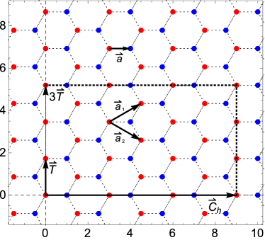
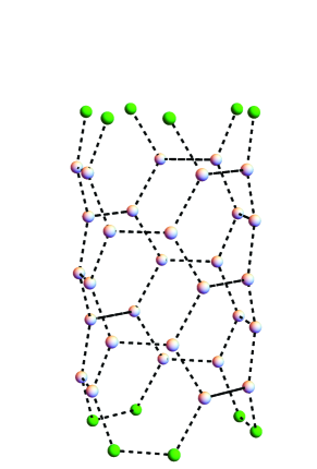
Figure 1: Construction of nanotubes from a planar hexagonal lattice. The left panel shows the hexagonal lattice from which the tubes are formed. The vectors $\vec{T}$ and $\vec{C}_{h}$ are shown for the $(3,3)$ chirality. Also shown are the hexagonal unit vectors $\vec{a}_{1}$ and $\vec{a}_{2}$. The hexagonal lattice can be described in terms of two triangular lattices A and B (colored red and blue, respectively) shifted by the vector $\vec{a}$. The rectangle defined by the vectors $\vec{C}_{h}$ and $3\vec{T}$ can be cut and rolled along the longitudinal direction to form a nanotube with $N_{L}=3$, shown in the right panel. The ends of the tube are identified, due to the periodic boundary conditions applied in the longitudinal direction.

We shall first review the construction of nanotubes from a planar hexagonal lattice, with emphasis on the “(3,3) nanotube” which we shall later use in our lattice Monte Carlo calculations. The geometry of the (3,3) nanotube can be obtained by first considering a planar graphene (honeycomb) lattice, shown in the left panel of Fig. 1. Each point on the graphene lattice can be obtained by integer combinations of the unit vectors

$$\vec{a}_{1} \equiv \left(\frac{3}{2},\frac{\sqrt{3}}{2}\right)a\ ,$$ (1)

$$\vec{a}_{2} \equiv \left(\frac{3}{2},-\frac{\sqrt{3}}{2}\right)a\ ,$$ (2)

where $a=1.42$ Å is the physical lattice spacing (lattice constant) of graphene. We find

$$\vec{b}_{1} \equiv \left(\frac{1}{3},\frac{1}{\sqrt{3}}\right)\frac{2\pi}{a}\ ,$$ (3)

$$\vec{b}_{2} \equiv \left(\frac{1}{3},-\frac{1}{\sqrt{3}}\right)\frac{2\pi}{a}\ .$$ (4)

for the reciprocal lattice vectors. The hexagonal lattice can also be described in terms of two triangular lattices (labeled A and B), separated by the vector $\vec{a}\equiv(\vec{a}_{1}+\vec{a}_{2})/3$ as shown in Fig. 1. Such a description of the graphene lattice will be useful for our path integral formulation in Section III.

A general nanotube of “chirality” $(n,m)$ is given in terms of the “chiral vector” $\vec{C}_{h}$,

$$\vec{C}_{h}\equiv n\vec{a}_{1}+m\vec{a}_{2},$$ (5)

where $n$, $m$ are integers with $0\leq|m|\leq n$. The “translation vector” $\vec{T}$ perpendicular to the chiral vector $\vec{C}_{h}$ is defined as

$$\vec{T}\equiv t_{1}\vec{a}_{1}+t_{2}\vec{a}_{2},$$ (6)

with

$$t_{1} \equiv \frac{2m+n}{d_{R}}$$ (7)

$$t_{2} \equiv -\frac{2n+m}{d_{R}},$$ (8)

where $d_{R}\equiv\mathrm{gcd}(2m+n,2n+m)$ (greatest common divisor). These vectors are shown in Fig. 1 for the case of $(n,m)=(3,3)$.

In order to construct a $(3,3)$ nanotube, we cut from the graphene lattice the rectangle formed by the chiral and translation vectors. Next, we roll the rectangle along the $\vec{C}_{h}$ vector, in order to form a nanotube. Thus, we identify $\vec{C}_{h}$ as the vector that points along the circumferential direction of the tube, while the vector $\vec{T}$ points along the longitudinal direction of the tube. This construction represents one “unit cell” of a nanotube of length $|\vec{T}|$. The number of hexagons $N$ within this nanotube unit is

$$N_{U}=\frac{|\vec{C}_{h}\times\vec{T}|}{|\vec{a}_{1}\times\vec{a}_{2}|},$$ (9)

and for the $(3,3)$ tube, this gives $N_{U}=6$ and $|\vec{T}|=\sqrt{3}a$.

The length of the tube can be increased by adding additional unit cells to its ends. We denote by $N_{L}$ the number of unit cells along the longitudinal direction, giving an overall tube length of $N_{L}|\vec{T}|$ and a total number of hexagons $N_{L}N_{U}$. In our lattice Monte Carlo studies of the $(3,3)$ nanotube, we use $N_{L}$ = 3, 6, and 9. In the right panel of Fig. 1, we show a $(3,3)$ tube with $N_{L}=3$ unit cells. In Table 1 we summarize the other properties of the nanotubes under consideration.

Table 1: Overview of the properties of the (3,3) nanotubes used in our lattice Monte Carlo calculations. All lengths are given in units of the graphene lattice constant $a=1.42$ Å.

$N_{L}$	diameter $|\vec{C}_{h}|/\pi$	length $N_{L}|\vec{T}|$	# of hexagons $N=N_{L}N_{U}$	# of ions
1	9/$\pi$	$\sqrt{3}\ (=|\vec{T}|)$	$6\ (=N_{U})$	12
3	9/$\pi$	$3\sqrt{3}$	18	36
6	9/$\pi$	$6\sqrt{3}$	36	72
9	9/$\pi$	$9\sqrt{3}$	54	108

III Path Integral Formalism

We note that detailed treatments of the path integral formalism for a graphene monolayer in the tight-binding description have already been given in Refs. Brower et al. (2011); Smith and von Smekal (2014). Hence, our main objectives are to give a cursory overview intended to introduce notation, and to highlight the differences encountered in the application to carbon nanotubes. The Hamiltonian $H$ of the carbon nanotube system consists of the tight binding Hamiltonian $H_{tb}$ that describes the interaction of the electrons with the carbon ions, and of the interaction Hamiltonian $H_{I}$, responsible for electron-electron correlations. We write this in the form

$$H \equiv H_{tb}+H_{I}$$

$$\equiv -\kappa\sum_{\langle x,y\rangle,s}a^{\dagger}_{x,s}a_{y,s}+\frac{1}{2}\sum_{x,y}V_{x,y}\,q_{x}q_{y},$$

where $x$ and $y$ denote sites on the honeycomb lattice, $\kappa\simeq 2.7$ eV is the nearest-neighbor hopping amplitude for electrons in graphene, and $V_{x,y}$ is the electron-electron potential matrix (see Section V.1). Further, $\langle x,y\rangle$ denotes summation over nearest neighbors, and $s$ assumes the values ($\uparrow$, “spin up”) or ($\downarrow$, “spin down”). Also, $q_{i}\equiv a^{\dagger}_{i,\uparrow}a_{i,\uparrow}+a^{\dagger}_{i,\downarrow}a_{i,\downarrow}-1$ is the charge operator at position $i$, shifted by ($-1$) to ensure overall neutrality (“half-filling”). In contrast to Ref. Smith and von Smekal (2014), we do not introduce a “staggered mass” term to our Hamiltonian (see Eqn. 10 of Ref. Smith and von Smekal (2014)). As mentioned in the introduction, we do not include the effects of curvature in our Hamiltonian, which induces geometrical tilting of $\pi$ orbitals and hybridization of $\sigma$ bonds Blase et al. (1994). We note that the effects of curvature can be incorporated into our calculations by using hopping parameters that are dependent on the direction of the three nearest neighbor bonds relative to the tube and azimuthal directions, i.e., $\kappa_{i}$ for $i=1,2,3$, as described in Kleiner and Eggert (2001).

In order to recast the Hamiltonian in a form more amenable to Quantum Monte Carlo calculations, we define the “hole” operators for spin $\downarrow$ electrons,

$$b^{\dagger}_{x,\downarrow}\equiv a_{x,\downarrow},\qquad b_{x,\downarrow}\equiv a^{\dagger}_{x,\downarrow},$$ (11)

and similarly for spin $\uparrow$ electrons. In terms of these new operators, Eqn. (III) becomes

$$H=-\kappa\sum_{\langle x,y\rangle}\left(a^{\dagger}_{x,\uparrow}a_{y,\uparrow}-b^{\dagger}_{x,\downarrow}b_{y,\downarrow}\right)+\frac{1}{2}\sum_{x,y}V_{x,y}\,q_{x}q_{y},$$ (12)

with the charge operator $q_{i}=a^{\dagger}_{i,\uparrow}a_{i,\uparrow}-b^{\dagger}_{i,\downarrow}b_{i,\downarrow}$. Finally, we flip the sign of the operators $b$ and $b^{\dagger}$ on one of the sublattices. This impacts only the nearest-neighbor hopping term of the Hamiltonian and leaves the dynamics of the system invariant, as the anticommutation relations of the hole operators remain unchanged. However, this last step is essential in ensuring a positive definite probability measure for our Monte Carlo calculations, as we shall discuss below. The Hamiltonian now becomes

$$H=-\kappa\sum_{\langle x,y\rangle}\left(a^{\dagger}_{x}a_{y}+b^{\dagger}_{x}b_{y}\right)+\frac{1}{2}\sum_{x,y}V_{x,y}\,q_{x}q_{y},$$ (13)

where the superfluous spin indices have been dropped.

The basis of our Monte Carlo calculations is Eqn. (13), and we are interested in calculating expectation values of operators $O$ (or time-ordered products of operators),

$$\langle O(t)\rangle\equiv\frac{1}{Z}\text{Tr}\left[O(t)e^{-\beta H}\right]\\ =\frac{1}{Z}\int\left[\prod_{\alpha}d\psi^{*}_{\alpha}d\psi_{\alpha}d\eta^{*}_{\alpha}d\eta_{\alpha}\right]e^{-\sum_{\alpha}(\psi^{*}_{\alpha}\psi_{\alpha}+\eta^{*}_{\alpha}\eta_{\alpha})}\langle-\psi,-\eta|O(t)e^{-\beta H}|\psi,\eta\rangle,$$ (14)

where $Z\equiv\mathrm{Tr}\left[e^{-\beta H}\right]$ is the partition function. The Grassmann-valued fields $\psi$ and $\eta$ represent electrons and holes, respectively. Their products and sums (denoted by $\alpha$) are over all fermionic degrees of freedom. Here, $\beta$ is an inverse temperature and is identified with the temporal extent of our system.

If we now divide $e^{-\beta H}$ into $N_{t}$ “time slices” according to

$$e^{-\beta H}\equiv e^{-\delta H}e^{-\delta H}\cdot\cdot\cdot e^{-\delta H},$$ (15)

where $\delta\equiv\beta/N_{t}$, we may insert a complete set of fermionic coherent states,

$$\openone=\int\left[\prod_{\alpha}d\psi^{*}_{\alpha}d\psi_{\alpha}d\eta^{*}_{\alpha}d\eta_{\alpha}\right]e^{-\sum_{\alpha}(\psi^{*}_{\alpha}\psi_{\alpha}+\eta^{*}_{\alpha}\eta_{\alpha})}|\psi,\eta\rangle\langle\psi,\eta|,$$

between each of the factors on the RHS of Eqn. (15). One then arrives at the following expression for the partition function,

$$Z=\text{Tr}\left[e^{-\beta H}\right]=\\ \int\prod_{t=0}^{N_{t}-1}\left\{\left[\prod_{\alpha}d\psi^{*}_{\alpha,t}d\psi_{\alpha,t}d\eta^{*}_{\alpha,t}d\eta_{\alpha,t}\right]e^{-\sum_{\alpha}(\psi^{*}_{\alpha,t+1}\psi_{\alpha,t+1}+\eta^{*}_{\alpha,t+1}\eta_{\alpha,t+1})}\langle\psi_{t+1},\eta_{t+1}|e^{-\delta H}|\psi_{t},\eta_{t}\rangle\right\},$$ (16)

which depends on the Grassmann fields only. In order to account for the minus sign in the Grassmann fields generated by the trace in Eqn. (14), we identify $\psi_{N_{t}}=-\psi_{0}$ and $\eta_{N_{t}}=-\eta_{0}$, which corresponds to anti-periodic boundary conditions in the temporal dimension.

We now introduce an “auxiliary field” $\phi$ by means of a Hubbard-Stratonovich (HS) transformation in the matrix element on the RHS of Eqn. (16),

$$\langle\psi_{t+1},\eta_{t+1}|e^{-\delta H}|\psi_{t},\eta_{t}\rangle=\langle\psi_{t+1},\eta_{t+1}|e^{\delta\kappa\sum_{\langle x,y\rangle}\left(a^{\dagger}_{x}a_{y}+b^{\dagger}_{x}b_{y}\right)-\frac{1}{2}\sum_{x,y}\delta V_{x,y}q_{x}q_{y}}|\psi_{t},\eta_{t}\rangle\\ \propto\int\prod_{x}d\tilde{\phi}_{x}\langle\psi_{t+1},\eta_{t+1}|e^{\tilde{\kappa}\sum_{\langle x,y\rangle}\left(a^{\dagger}_{x}a_{y}+b^{\dagger}_{x}b_{y}\right)-\frac{1}{2}\sum_{x,y}[\tilde{V}]^{-1}_{x,y}\tilde{\phi}_{x}\tilde{\phi}_{y}+\sum_{x}i\tilde{\phi}_{x}q_{x}}|\psi_{t},\eta_{t}\rangle,$$ (17)

where we have introduced the dimensionless variables

$$\tilde{\kappa}\equiv\delta\kappa,\quad\tilde{V}\equiv\delta V,\quad\tilde{\phi}\equiv\delta\phi,$$

and we note that Eqn. (17) is valid up to an irrelevant overall constant and rescaling. We note that the stability of this transformation in a Monte Carlo calculation relies on $V_{x,y}^{-1}$ being positive definite.

We now apply the identity Luscher (1977)

$$\langle\psi|\exp\left\{\sum_{x,y}a^{\dagger}_{x}A_{x,y}a_{y}\right\}|\psi^{\prime}\rangle\equiv\exp\left\{\sum_{x,y}\psi^{*}_{x}[e^{A}]_{x,y}\psi^{\prime}_{y}\right\},$$ (18)

where $A_{x,y}$ is a matrix of c-numbers, to the interaction term. We then obtain Buividovich and Polikarpov (2012); Ulybyshev et al. (2013)

$$\langle\psi_{t+1},\eta_{t+1}|e^{-\delta H}|\psi_{t},\eta_{t}\rangle=\int\prod_{x}d\tilde{\phi}_{x,t}\,e^{-\frac{1}{2}\sum_{x,y}[\tilde{V}]^{-1}_{x,y}\tilde{\phi}_{x,t}\tilde{\phi}_{y,t}}\\ \times\exp\left\{\tilde{\kappa}\sum_{\langle x,y\rangle}\left(\psi^{*}_{x,t+1}\psi_{y,t}+\eta^{*}_{x,t+1}\eta_{y,t}\right)+\sum_{x}\left(e^{i\tilde{\phi}_{x,t}}\psi^{*}_{x,t+1}\psi_{x,t}+e^{-i\tilde{\phi}_{x,t}}\eta^{*}_{x,t+1}\eta_{x,t}\right)\right\}+\mathcal{O}(\delta^{2}),$$ (19)

where we have introduced a “time index” $t$ for the auxiliary field $\phi_{x,t}$. If we insert this expression into Eqn. (16), we find

$$Z=\int\mathcal{D}\tilde{\phi}\mathcal{D}\psi^{*}\mathcal{D}\psi\mathcal{D}\eta^{*}\mathcal{D}\eta\,e^{-\frac{1}{2}\sum_{x,y,t}[\tilde{V}]^{-1}_{x,y}\tilde{\phi}_{x,t}\tilde{\phi}_{y,t}}\exp\bigg{\{}\tilde{\kappa}\sum_{\langle x,y\rangle,t}\left(\psi^{*}_{x,t+1}\psi_{y,t}+\eta^{*}_{x,t+1}\eta_{y,t}\right)\\ -\sum_{x,t}\left(\psi^{*}_{x,t+1}(\psi_{x,t+1}-e^{i\tilde{\phi}_{x,t}}\psi_{x,t})+\eta^{*}_{x,t+1}(\eta_{x,t+1}-e^{-i\tilde{\phi}_{x,t}}\eta_{x,t})\right)\bigg{\}},$$ (20)

where $\mathcal{D}\tilde{\phi}$ is a shorthand notation for $\prod_{x,t=0}^{N_{t}-1}d\tilde{\phi}_{x,t}$ (and similarly for the other fields). The motivation for the HS transformation is now clear: Only quadratic powers of the fermion fields appear in the argument of the exponent (without the HS transformation, quartic powers would also appear). We are now in a position to perform the Gaussian-type integrals over the fermion fields. Up to irrelevant overall factors, the partition function becomes

$$Z=\int\mathcal{D}\tilde{\phi}\det[M(\tilde{\phi})]\det[M^{*}(\tilde{\phi})]\exp\left\{-\frac{1}{2}\sum_{x,y,t=0}^{N_{t}-1}[\tilde{V}]^{-1}_{x,y}\tilde{\phi}_{x,t}\tilde{\phi}_{y,t}\right\},$$ (21)

where the fermion matrix $M$ is a functional of $\tilde{\phi}$,

$$M(x,t;y,t^{\prime};\tilde{\phi})\equiv\delta_{x,y}\left(\delta_{t,t^{\prime}}-e^{i\tilde{\phi}_{x,t^{\prime}}}\delta_{t-1,t^{\prime}}\right)-\tilde{\kappa}\,\delta_{\langle x,y\rangle}\delta_{t-1,t^{\prime}},$$ (22)

where $\delta_{\langle x,y\rangle}$ equals unity if $x$ and $y$ are nearest-neighbor sites, and zero otherwise. This is referred to as the “compact formulation” of the path integral for the interacting, hexagonal tight-binding system.

The feasibility of a Monte Carlo evaluation of the path integral relies on the generation of configurations of $\tilde{\phi}$ that follow the probability distribution

$$P(\tilde{\phi}) \equiv \frac{1}{Z}\det[M(\tilde{\phi})]\det[M^{*}(\tilde{\phi})]\exp\left\{-\frac{1}{2}\sum_{x,y,t=0}^{N_{t}-1}[\tilde{V}]^{-1}_{x,y}\tilde{\phi}_{x,t}\tilde{\phi}_{y,t}\right\}$$ (23)

$$= \frac{1}{Z}\det[M(\tilde{\phi})M^{\dagger}(\tilde{\phi})]\exp\left\{-\frac{1}{2}\sum_{x,y,t=0}^{N_{t}-1}[\tilde{V}]^{-1}_{x,y}\tilde{\phi}_{x,t}\tilde{\phi}_{y,t}\right\},$$ (24)

which is positive definite as long as $V^{-1}_{x,y}$ is positive definite. Also, $\det[M(\tilde{\phi})M^{\dagger}(\tilde{\phi})]\geq 0$ for any $\phi$. We use global Hybrid Monte Carlo (HMC) lattice updates in order to generate the necessary ensembles of configurations, which we denote by $\{\tilde{\phi}\}$. For a thorough discussion of the HMC algorithm and related issues, see for example Refs. Smith and von Smekal (2014); Gattringer and Lang (2009). Given an ensemble $\{\tilde{\phi}\}$, the Monte Carlo estimate of the expectation value of any operator $O$ is given by

$$\langle O\rangle\approx\frac{1}{N_{\mathrm{cf}}}\sum_{i=1}^{N_{\mathrm{cf}}}O[\tilde{\phi_{i}}],$$ (25)

where $\tilde{\phi}_{i}\in\{\tilde{\phi}\}$ and $N_{\mathrm{cf}}$ is the number of configurations within the ensemble. Each such estimate carries with it an associated uncertainty which (in principle) can be arbitrarily reduced with increased statistics (i.e. by taking $N_{\mathrm{cf}}\rightarrow\infty$). In this first study, we are interested in computing the single quasi-particle spectrum, which can be accessed by taking $O=a_{x}(\tau)a^{\dagger}_{y}(0)$,

$$\langle a_{x}(\tau)a^{\dagger}_{y}(0)\rangle=\langle M^{-1}(x,\tau;y,0)\rangle\approx\frac{1}{N_{\mathrm{cf}}}\sum_{i=1}^{N_{\mathrm{cf}}}M^{-1}(x,\tau;y,0;\tilde{\phi}_{i}),$$ (26)

and by analyzing the temporal behavior of the resulting correlator.

We finally note that the fermion fields can be recast in terms of two-component fields, with one component for the underlying $A$ sublattice and the other one for the $B$ sublattice. For instance, the electron fields can be written as

$$\Psi(x,t)=\begin{pmatrix}\Psi_{A}(x,t)\\ \Psi_{B}(x,t)\end{pmatrix}=\begin{pmatrix}\psi_{x,t}\\ \psi_{x+\vec{a},t}\end{pmatrix},$$ (27)

where $x$ in this case represents the location of a given hexagonal unit cell. In this manner, the ion on site $A$ associated with this particular hexagonal unit cell is located at position $x$, while the ion on site $B$ is located at $x+\vec{a}$. An analogous definition can be made for the auxiliary HS field,

$$\Phi(x,t)=\begin{pmatrix}\Phi_{A}(x,t)\\ \Phi_{B}(x,t)\end{pmatrix}=\begin{pmatrix}\tilde{\phi}_{x,t}\\ \tilde{\phi}_{x+\vec{a},t}\end{pmatrix},$$ (28)

and the matrix $M(x,t^{\prime};y,t)$ acting on the two-component fermion field is now given by

$$M(x,t^{\prime};y,t)\Psi(y,t)=\\ \begin{pmatrix}\delta_{x,y}\left(\delta_{t^{\prime},t}-e^{i\Phi_{A}(x,t^{\prime})}\delta_{t-1,t^{\prime}}\right)&-\tilde{\kappa}\ \delta_{\langle x,y\rangle}\delta_{t-1,t^{\prime}}\\ -\tilde{\kappa}\ \delta_{\langle x,y\rangle}\delta_{t-1,t^{\prime}}&\delta_{x,y}\left(\delta_{t^{\prime},t}-e^{i\Phi_{B}(x,t^{\prime})}\delta_{t-1,t^{\prime}}\right)\end{pmatrix}\begin{pmatrix}\Psi_{A}(y,t)\\ \Psi_{B}(y,t)\end{pmatrix},$$ (29)

where the coordinates $x$ and $y$ now represent locations of hexagonal unit cells (and not of the ions themselves), so that the definition of $\delta_{\langle x,y\rangle}$ must be slightly modified to account for all pairs of unit cell locations $x$ and $y$ that share nearest neighbor ions. While we stress that the matrix notation for $M(x,y;t)$ in Eqn. (29) is equivalent to Eqn. (22), the underlying $A/B$ sublattice structure has now been made explicit. We find this representation convenient in analyzing the non-interacting limit of our theory, as discussed Section IV, and also in our zero-mode analysis in Section V.3 and Appendix A.

IV Non-interacting system

Before we present results of calculations that include electron-electron correlations, it is highly instructive to recall the non-interacting (tight-binding) theory and to compare with the results of our path-integral calculations in this regime. Not only does this exercise allow us to emphasize some salient features of our formalism, but it also allows us to find an accurate way of representing temporal finite differences on the lattice in a way which avoids the infamous “doubling problem”, where spurious high-momentum modes contribute in the continuum limit.

IV.1 Zero-temperature continuum limit

The non-interacting case is obtained by setting $\tilde{\phi}=0$ in our expressions for the path integral. In the $\delta\rightarrow 0$ (continuous time) limit, it is straightforward to show that Eqn. (29) becomes

$$M(x,y;t)\Psi(y;t)=\begin{pmatrix}\delta_{x,y}\ \partial_{t}&-\kappa\ \delta_{\langle x,y\rangle}\\ -\kappa\ \delta_{\langle x,y\rangle}&\delta_{x,y}\ \partial_{t}\end{pmatrix}\begin{pmatrix}\Psi_{A}(y,t)\\ \Psi_{B}(y,t)\end{pmatrix},$$ (30)

when expressed in terms of dimensionful quantities. We shall first consider the zero-temperature limit, followed by the case of finite temperature. We now move to Fourier space in the $\beta\rightarrow\infty$ (zero temperature) limit, expressing Eqn. (30) as

$$M(x,y;t)=\frac{1}{2\pi}\int_{-\infty}^{\infty}d\omega\,e^{i\omega t}\frac{1}{N_{U}}\sum_{i=0}^{N_{U}-1}\frac{|\vec{T}|}{2\pi}\int d\vec{k}_{||}e^{i(\vec{k}_{||}+\vec{k}_{\bot,i})\cdot(\vec{x}-\vec{y})}\,\widetilde{M}(\vec{k}_{\bot}+\vec{k}_{\bot,i};\omega),$$ (31)

where

$$\widetilde{M}(\vec{k};\omega)=\begin{pmatrix}i\omega&-\kappa f(\vec{k})\\ -\kappa f^{*}(\vec{k})&i\omega\end{pmatrix},$$ (32)

and

$$f(\vec{k})=e^{iak_{x}/\sqrt{3}}+2e^{-iak_{x}/(2\sqrt{3})}\cos(ak_{y}/2),$$ (33)

following Ref. Saito et al. (1998). In Eqn. (31) we have introduced the momentum variables $\vec{k}_{||}$ and $\vec{k}_{\bot,i}$ which satisfy

$$\vec{k}_{||}\cdot\vec{k}_{\bot,i}=0\quad,\quad\vec{T}\cdot\vec{k}_{\bot,i}=0\ ,$$

where $\vec{T}$ (Eqn. (6)) is parallel to the tube axis. Since we assume that the tube is infinitely long, $\vec{k}_{||}$ is continuous within an interval of length $2\pi/|\vec{T}|$. However, the momentum $\vec{k}_{\bot}$ is discrete due to the finite circumference of the tube. These discrete momenta $\vec{k}_{\bot,j}$ are given by Saito et al. (1998)

$$\vec{k}_{\bot,j}\equiv\frac{j}{N_{U}}(t_{1}\vec{b}_{2}-t_{2}\vec{b}_{1}),$$ (34)

where the $t_{i}$ are translation vector components and $\vec{b}_{i}$ the reciprocal lattice vectors, as discussed in Section II. Also, $N_{U}$ is given by Eqn. (9) and $j\in[0,N_{U}-1]$.

To determine the zero-temperature dispersion relation for a single quasiparticle in the non-interacting limit, it suffices to study the pole structure of $\widetilde{M}^{-1}$. This is equivalent to finding simultaneous values of $\omega$ and $\vec{k}$ that satisfy the quantization condition

$$\det[\widetilde{M}(\vec{k};\omega)]=0,$$ (35)

which admits the solution

$$E(\vec{k})=i\omega(\vec{k})=\pm\kappa|f(\vec{k})|,$$ (36)

for the energy $E(\vec{k})$ of the quasiparticle. In Fig. 2, we show the dispersion relation as function of $\vec{k}_{||}$ for the $(3,3)$ tube. Because of the discrete momenta perpendicular to the tube direction, the dispersion relation consists of bands of energy curves. Note that the point with the largest magnitude of the energy occurs at the $\Gamma$ point $(|k_{||}|,|k_{\bot,i}|)=(0,0)$, while the zero-energy Dirac point $K$ occurs at non-zero momentum $|\vec{T}|(|k_{||}|,|k_{\bot,i}|)=(\frac{2\pi}{3},\frac{2\pi}{\sqrt{3}})$.

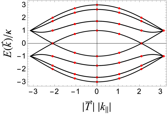
Figure 2: Non-interacting (tight-binding) dispersion relation for a $(3,3)$ nanotube of infinite length (solid black lines) and one with $N_{L}=6$ unit cells (red points). The abscissa shows the momentum $|\vec{T}||k_{||}|$ parallel to the tube axis, while the ordinate shows the energy (in units of $\kappa$) for a single quasiparticle. Positive energies denote particles, and negative energies denote holes.

IV.2 Dispersion for a tube of finite length

For reasons of computational practicality, our Monte Carlo calculations are performed with tubes of finite length, with periodic boundary conditions at the ends of the tube. As shown in the right panel of Fig. 1, the top (green) lattice points are (from the point of view of the Monte Carlo calculation) identical to the bottom (green) lattice points, by virtue of the periodic boundary conditions. This implies that the momenta $\vec{k}_{||}$ in the direction parallel to the tube axis will also be discrete, with wave vectors separated by $2\pi/(N_{L}|\vec{T}|)$, where $N_{L}|\vec{T}|$ is the overall tube length. For the non-interacting case, the dispersion relation becomes a series of points that coincide with the continuous lines shown in Fig. 2. The density of points and the exact functional form of the lines depends on the length and chirality of the tube.

In Fig. 2, the discrete dispersion points are shown for the specific case of the $(3,3)$ tube with $N_{L}=6$ unit cells. It should be noted that some of these coincide with the Dirac K points. A shift of the energy away from this point (for instance due to interactions) would indicate the existence of an energy gap at the Dirac point. In general, given an $(n,m)$ tube that exhibits a Dirac point, the number of unit cells should be a multiple of three in order for the discrete dispersion to access the Dirac point Saito et al. (1998). In other words, the discrete momentum modes should include a subset of $|\vec{T}|(|k_{||}|,|k_{\bot,i}|)=(\frac{2\pi}{3},\frac{2\pi}{\sqrt{3}})$ and/or $|\vec{T}|(|k_{||}|,|k_{\bot,i}|)=(0,\frac{4\pi}{3})$. This condition is the reason why we focus on tubes with $N_{L}=3$, 6, and 9 unit cells.

IV.3 Finite temperature

In addition to calculations with a finite tube length, the path integral formalism requires the introduction of a finite temporal extent $\beta$ (as discussed in Section III), which in turn can be viewed as an inverse temperature. This implies that the frequency integral should be replaced by the summation

$$\frac{1}{2\pi}\int_{-\infty}^{\infty}d\omega\ e^{i\omega\tau}\rightarrow\frac{1}{\beta}\sum_{n=-\infty}^{\infty}e^{i\omega_{n}\tau}\ ,$$ (37)

where

$$\omega_{n}\equiv\frac{2\pi}{\beta}\left(n+\frac{1}{2}\right),$$ (38)

are the Matsubara frequencies. We note that the expression for the correlator

$$G(\vec{k}_{i},\tau)\equiv\frac{1}{\beta}\sum_{n=-\infty}^{\infty}\ e^{i\omega_{n}t}\ \widetilde{M}^{-1}(\vec{k}_{i};\omega_{n}),$$ (39)

can be evaluated analytically using straightforward (though tedious) algebra. In the range $0<\tau<\beta$, we find

$$G(\vec{k}_{i},\tau) = \frac{1}{2\cosh(\omega(\vec{k}_{i})\beta/2)}\begin{pmatrix}\cosh(\omega(\vec{k}_{i})(\tau-\beta/2))&e^{i\theta_{k_{i}}}\sinh(\omega(\vec{k}_{i})(\tau-\beta/2))\\ e^{-i\theta_{k_{i}}}\sinh(\omega(\vec{k}_{i})(\tau-\beta/2))&\cosh(\omega(\vec{k}_{i})(\tau-\beta/2))\end{pmatrix}\quad$$ (40)

$$\equiv \begin{pmatrix}G_{AA}(\vec{k}_{i},\tau)&G_{AB}(\vec{k}_{i},\tau)\\ G_{BA}(\vec{k}_{i},\tau)&G_{BB}(\vec{k}_{i},\tau)\end{pmatrix},$$ (41)

where $G_{BA}(\vec{k}_{i},\tau)=G^{*}_{AB}(\vec{k}_{i},\tau)$,

$$\theta_{k_{i}}\equiv\tan^{-1}(\text{Im}f(\vec{k}_{i})/\text{Re}f(\vec{k}_{i})),$$ (42)

and $\omega(\vec{k}_{i})$ is given by the positive solution in Eqn. (36). The form of Eqn. (41) is due to the underlying $A/B$ sublattice structure, and admits two linearly independent correlator solutions (see for instance Ref. Terakura and Akai (2013)),

$$G_{\pm}(\vec{k}_{i},\tau) \equiv \frac{1}{2}\left[G_{AA}(\vec{k}_{i},\tau)+G_{BB}(\vec{k}_{i},\tau)\pm(G_{AB}(\vec{k}_{i},\tau)+G_{BA}(\vec{k}_{i},\tau))\right]$$ (43)

$$= \frac{1}{2\cosh(\omega(\vec{k}_{i})\beta/2)}\left[\cosh(\omega(\vec{k}_{i})(t-\beta/2))\pm\cos(\theta_{k_{i}})\sinh(\omega(\vec{k}_{i})(t-\beta/2))\right],\quad$$ (44)

which for $t\ll\beta$ behave as

$$G_{\pm}(\vec{k}_{i},\tau)\propto e^{\pm\omega(\vec{k}_{i})\tau},$$ (45)

which shows that the “leading” exponential behavior of these correlators provides access to the (non-interacting) spectrum of the theory. As we show in Section VI, we use this aspect of the correlators when we compute the spectrum in the presence of electron-electron correlations.

IV.4 Discretization of time

We now consider the case where the temporal dimension is also discretized. Given a temporal extent $\beta$ divided into $N_{t}$ time steps of equal width $\delta=\beta/N_{t}$, the allowed Matsubara frequencies $\omega_{n}=\frac{2\pi}{T}(n+1/2)$ are those that fall within the first Brillouin zone $[-\pi/\delta,\pi/\delta)$, which corresponds to $-N_{t}/2\leq n<N_{t}/2$. The time derivative in Eqn. (30) should now be approximated using these discrete steps. As we show below, analytic expressions are still obtainable for the non-interacting case. In what follows, we make use of the representation,

$$\delta_{t_{i},t_{j}}=\frac{1}{N_{t}}\sum_{n=-N_{t}/2}^{N_{t}/2-1}e^{i\omega_{n}(t_{i}-t_{j})},$$ (46)

where $t_{i}=i\delta$ and $t_{j}=j\delta$ are lattice time sites ($i$ and $j$ are integers with $0\leq i,j<N_{t}$).

IV.4.1 Forward difference

We first consider the case of forward discretization to approximate the derivative

$$\partial_{\tau}f(t) \rightarrow \frac{1}{\delta}\left(\delta_{\tau+\delta,t}-\delta_{\tau,t}\right)f(t)$$ (47)

$$= \frac{1}{N_{t}\delta}\left(\sum_{n}e^{i\omega_{n}(\tau+\delta-t)}-\sum_{n}e^{i\omega_{n}(\tau-t)}\right)f(t)$$ (48)

$$= \frac{1}{N_{t}}\sum_{n}e^{i\omega_{n}(\tau-t)}\frac{1}{\delta}e^{i\omega_{n}\delta/2}\left(e^{i\omega_{n}\delta/2}-e^{-i\omega_{n}\delta/2}\right)f(t)$$ (49)

$$= \frac{1}{N_{t}}\sum_{n}e^{i\omega_{n}(\tau-t)}\frac{2i}{\delta}e^{i\omega_{n}\delta/2}\sin(\omega_{n}\delta/2)f(t),$$ (50)

where $f(t)$ is an arbitrary function on the lattice. Under this differencing scheme, the matrix $\widetilde{M}$ in Eqn. (30) in the momentum-frequency domain becomes

$$\widetilde{M}(\vec{k};\omega_{n})=\begin{pmatrix}\frac{2i}{\delta}e^{i\omega_{n}\delta/2}\sin(\omega_{n}\delta/2)&-\kappa f(\vec{k})\\ -\kappa f^{*}(\vec{k})&\frac{2i}{\delta}e^{i\omega_{n}\delta/2}\sin(\omega_{n}\delta/2)\end{pmatrix},$$ (51)

for which the quantization condition

$$\det(\widetilde{M}(\vec{k};\omega_{n}))=0\ ,$$ (52)

gives the solution

$$\omega_{n}^{2}(1+i\omega_{n}\delta)+\mathcal{O}(\delta^{2})=-\kappa^{2}|f(\vec{k})|^{2},$$ (53)

for small $\delta$. Hence, we expect our energies computed in this discretized scheme to be shifted by $\mathcal{O}(\delta)$ from the result in the (temporal) continuum limit. We note that for a backward time difference

$$\partial_{\tau}f(t)\rightarrow\frac{1}{\delta}\left(-\delta_{\tau-\delta,t}+\delta_{\tau,t}\right)f(t),$$ (54)

an analogous derivation gives similar results, provided that the replacement $i\omega_{n}\rightarrow-i\omega_{n}$ is made in Eqs. (51) and (53).

IV.4.2 Mixed difference

Given our results for the forward and backward differences, a natural choice would be to consider a symmetric differencing scheme to approximate the time derivative according to

$$\partial_{\tau}f(t)\rightarrow\frac{1}{2\delta}\left(\delta_{\tau+\delta,t}-\delta_{\tau-\delta,t}\right)f(t),$$ (55)

although it is well know that this admits spurious high-energy solutions that have no analog in the continuum limit (see for instance the discussion on the “doubling problem” in Ref. Gattringer and Lang (2009)). Instead, we employ a “mixed” differencing scheme where we use a forward difference on $A$ sites and a backward difference on $B$ sites. We are free to do this, since the mixed scheme has the correct continuum limit. This idea was first pointed out in Ref. Brower et al. (2011), and we shall use it here for our non-interacting system. With mixed differencing, our fermion matrix becomes

$$\widetilde{M}(\vec{k};\omega_{n})=\begin{pmatrix}\frac{2i}{\delta}e^{i\omega_{n}\delta/2}\sin(\omega_{n}\delta/2)&-\kappa f(\vec{k})\\ -\kappa f^{*}(\vec{k})&\frac{2i}{\delta}e^{-i\omega_{n}\delta/2}\sin(\omega_{n}\delta/2)\end{pmatrix},$$ (56)

and the quantization condition gives

$$\omega_{n}^{2}+\mathcal{O}(\delta^{2})=-\kappa^{2}|f(\vec{k})|^{2},$$ (57)

which is “$\mathcal{O}(\delta)$ improved”, in comparison with Eqn. (53).

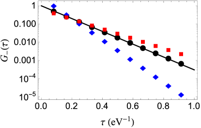
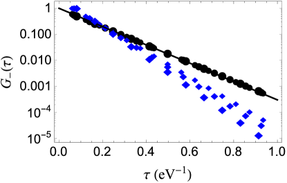
Figure 3: Comparison of analytic $G_{-}(\tau)$ correlator at the $\Gamma$ point (black line) to its discretized form. The left panel shows a calculation with $N_{t}=24$ discretized steps, where the (red) squares use the backward differencing scheme, (blue) diamonds use forward differencing scheme, and (black) circles use the mixed differencing scheme as described in text. The right panel shows the convergent behavior of the mixed and forward differencing schemes, with $N_{t}=24$, 28, and 32 timesteps. The decreasing pointsizes correspond to increasing $N_{t}$. Similar behavior is observed for the backward differencing scheme, but is not shown to reduce clutter. All calculations were performed with $\beta=2$ eV^-1.

We can visualize this improvement by direct inspection of the correlators. In Fig. 3, we compare the exact analytic correlator at the $\Gamma$ point to its discretized form, using the forward, backward, and mixed differencing schemes, noting that the time dependence of $\widetilde{M}$ is given by Eqn. (39). As can be seen from the left panel of Fig. 3, the mixed differencing scheme (black points) compares very well with the analytic result (black line) given by Eqn. (43), whereas the forward (blue diamonds) and backward (red squares) differencing schemes have clear systematic errors. These calculations were performed with $\beta=2$ eV^-1 and $N_{t}=24$ time steps. The right panel of Fig. 3 shows the convergence of the mixed and forward differencing schemes with increasing number of time steps: $N_{t}=24$, 28, and 32 (corresponding to decreasing symbol size). In this case, the improved convergence of the mixed differencing scheme is obvious, and indicates that extraction of spectra from the leading exponential behavior of the correlator is best done with the mixed differencing scheme. For the forward differencing scheme, we have confirmed that it does indeed converge to the analytical line as $N_{t}$ is increased. However, in order to get comparable results to the $N_{t}=24$ mixed-differencing scheme, the forward differencing scheme requires $N_{t}=256$ or larger. In the presence of interactions, the fermion matrix in the mixed-differencing scheme becomes

$$M(x,t^{\prime};y,t;\Phi)=\begin{pmatrix}\delta_{x,y}\left(e^{-i\Phi_{A}(x,t^{\prime})}\delta_{t+1,t^{\prime}}-\delta_{t,t^{\prime}}\right)&-\tilde{\kappa}\ \delta_{\langle x,y\rangle}\delta_{t,t^{\prime}}\\ -\tilde{\kappa}\ \delta_{\langle x,y\rangle}\delta_{t,t^{\prime}}&\delta_{x,y}\left(\delta_{t^{\prime},t}-e^{i\Phi_{B}(x,t^{\prime})}\delta_{t-1,t^{\prime}}\right)\end{pmatrix},$$ (58)

and we note that our use of this expression is motivated by the improved performance of the mixed-differencing scheme in the non-interacting case.

Since the conclusions of this section were obtained for the non-interacting system, it is not guaranteed that this $\mathcal{O}(\delta)$ improvement (or equivalently $\mathcal{O}(\delta^{2})$ scaling of results) persists in the presence of interactions. Recent studies related to explicit $\mathcal{O}(\delta^{2})$ differencing schemes in Ref. Buividovich et al. (2012); Smith and von Smekal (2014) suggest that the $\mathcal{O}(\delta)$ improvement is maintained in the presence of interactions, at least in the vicinity of the Dirac K point. As we show in Section VI.1, our results for the Dirac point support this finding as well. For dispersion points away from the Dirac point, our studies cannot definitively differentiate between $\mathcal{O}(\delta)$ or $\mathcal{O}(\delta^{2})$ scaling. However, for this initial study, we assume $\mathcal{O}(\delta^{2})$ scaling to perform our continuum limit extrapolations. Future calculations with additional values of $\delta$ should be able to clarify this scaling with certainty.

V Interacting system

Having considered the non-interacting system in some detail, we now turn to the case with electron-electron interactions. In Monte Carlo calculations of graphene, the electrons and holes propagate on the plane defined by the hexagonal graphene sheet, and thus the interaction between the particles is constructed to reflect this geometry. Furthermore, the spatial extent of the system in graphene calculations is typically much larger. In the case of a nanotube, interactions between particles can occur when they are, for example, on opposite sides of the tube wall. Thus, the interaction is not confined to a plane, and the construction of the potential matrix $V_{xy}$ depends on the chirality $(n,m)$ and length of the tube. We now turn to the construction of the potential.

V.1 Screened Coulomb potential

Our screened Coulomb interaction uses the results of RPA calculations performed by Wehling et al. Wehling et al. (2011) for the onsite interaction $U_{00}$, nearest neighbor $U_{01}$, next-to-nearest neighbor $U_{02}$, and next-to-next-to-nearest neightbor $U_{03}$ interaction. This interaction takes into account the short-distance screening due to the $\sigma$-band electrons (which are not dynamic in our calculations i.e. do not hop). We couple this interaction with a potential parameterized as in Smith and von Smekal (2014) that ensures the potential approaches the bare Coulomb potential at asymptotic distances. Translational invariance of the potential is maintained by employing a procedure similar to one described in Smith and von Smekal (2014): For any two points $\vec{x}$ and $\vec{y}$ on the nanotube, we determine within the tube the shortest distance $r$ between these two points with the ends of the tube identified by periodic boundary conditions. We then assign $V(r)$ as the potential matrix element $V_{xy}$ between these two points. Note that because of periodic boundary conditions at the ends of the tube, there will be cases when $r^{2}<(\vec{x}-\vec{y})^{2}$ since the largest value or $r_{||}$, the component of $r$ parallel to the tube direction, is $a|\vec{T}|N_{L}/2$. Due to the finite length of our tube calculations, the infrared divergence of the Coulomb potential is avoided. In Fig. 4 we show the matrix elements of the screened Coulomb potential used in our calculation of the $(3,3)$ tube with nine unit cells (points). For comparison, we also show the bare Coulomb potential evaluated at the same distances (triangles).

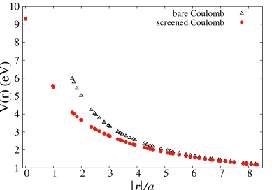
Figure 4: Screened Coulomb potential matrix elements (dots) used in our $(3,3)$ tube simulations with nine unit cells. For comparison, the triangles show the bare Coulomb potential evaluated at the same distances. The abscissa is plotted in units of the honeycomb lattice spacing.

V.2 Momentum projection

Unlike the non-interacting case, where the quasiparticle spectrum can be directly determined by analyzing the quantization conditions given by the determinant in Eqn. (35), the spectrum of the interacting system must be determined by analyzing the temporal behavior of the appropriate correlator. To access the spectrum at a particular momentum, we must first project our correlator to the corresponding momentum. Such a procedure is routinely performed in lattice QCD calculations. However, we discuss the formalism as it is applied to our system, in order to point out the specific differences to other lattice methods.

We denote the positions $\vec{x}_{i}$ of the unit cells of the tube collectively by $\{\vec{X}\}$. The momenta $\vec{k}_{i}$ conjugate to the unit cell cites are determined by the allowed reciprocal lattice vectors within the first Brillouin zone, which we denote collectively by $\{\vec{K}\}$. As our calculations use a finite number of unit cells, the allowed momenta in the $\vec{k}_{||}$ direction are also discrete, as discussed in Section IV.2. The unit cell positions and their conjugate momenta satisfy the orthogonality relations

$$\delta_{\vec{k}_{j},\vec{k}_{l}} = \frac{1}{N}\sum_{\vec{x}_{i}\in\{\vec{X}\}}e^{i\vec{x}_{i}\cdot(\vec{k}_{j}-\vec{k}_{l})},$$ (59)

$$\delta_{\vec{x}_{j},\vec{x}_{l}} = \frac{1}{N}\sum_{\vec{k}_{i}\in\{\vec{K}\}}e^{-i\vec{k}_{i}\cdot(\vec{x}_{j}-\vec{x}_{l})},$$ (60)

where $N$ is the number of unit cells (and not the number of ions). Given a function $f(\vec{x}_{i})$ of the unit cell coordinates, the above relations can be used to define its Fourier and inverse Fourier transforms

$$f(\vec{k}_{i}) \equiv \frac{1}{N}\sum_{\vec{x}_{j}\in\{\vec{X}\}}f(\vec{x}_{j})\,e^{i\vec{x}_{j}\cdot\vec{k}_{i}},$$ (61)

$$f(\vec{x}_{i}) \equiv \sum_{\vec{k}_{j}\in\{\vec{K}\}}\tilde{f}(\vec{k}_{i})\,e^{-i\vec{x}_{i}\cdot\vec{k}_{j}}.$$ (62)

In addition to the unit cell locations $\vec{x}_{i}$, each unit cell also includes a basis vector $\vec{a}$ due to the two underlying sublattices $A$ and $B$. This basis vector connects the $A$ site to the $B$ site within each unit cell. Given a unit cell position $\vec{x}$ and its basis vector $\vec{a}$, it is convenient to express creation operators in two-component form and with the following linear combinations,

$$a_{\pm}^{\dagger}(\vec{x})\equiv\frac{1}{\sqrt{2}}\begin{pmatrix}a^{\dagger}_{A}(\vec{x})\\ \pm a^{\dagger}_{B}(\vec{x})\end{pmatrix}=\frac{1}{\sqrt{2}}\begin{pmatrix}a^{\dagger}_{\vec{x}}\\ \pm a^{\dagger}_{\vec{x}+\vec{a}}\end{pmatrix}.$$ (63)

One can make an analogous definition for the hole operator $b^{\dagger}_{\pm}(\vec{x})$. In momentum space, the electron correlators are given by

$$G_{\pm}(\vec{k}_{i},\tau)\equiv\langle a_{\pm}(\vec{k}_{i},\tau)a_{\pm}^{\dagger}(\vec{k}_{i},0)\rangle=\frac{1}{N^{2}}\sum_{\vec{x}_{j},\vec{x}_{k}\in\{\vec{X}\}}e^{i\vec{k}_{i}\cdot(\vec{x}_{j}-\vec{x}_{k})}\langle a_{\pm}(\vec{x}_{j},\tau)a_{\pm}^{\dagger}(\vec{x}_{k},0)\rangle,$$ (64)

and by inserting Eqn. (63) into Eqn. (64), we find

$$G_{\pm}(\vec{k}_{i},\tau) = \frac{1}{2N^{2}}\sum_{\vec{x}_{j},\vec{x}_{k}\in\{\vec{X}\}}e^{i\vec{k}_{i}\cdot(\vec{x}_{j}-\vec{x}_{k})}\bigg{\{}\langle M^{-1}_{AA}(\vec{x}_{j},\vec{x}_{k};\tau)\rangle+\langle M^{-1}_{BB}(\vec{x}_{j},\vec{x}_{k};\tau)\rangle$$ (65)

$$\pm\left(\langle M^{-1}_{AB}(\vec{x}_{j},\vec{x}_{k};\tau)\rangle+\langle M^{-1}_{BA}(\vec{x}_{j},\vec{x}_{k};\tau)\rangle\right)\bigg{\}}$$

$$= \frac{1}{2}\left[G_{AA}(\vec{k}_{i},\tau)+G_{BB}(\vec{k}_{i},\tau)\pm(G_{AB}(\vec{k}_{i},\tau)+G_{BA}(\vec{k}_{i},\tau))\right],$$ (66)

where

$$G_{AB}(\vec{k}_{i},\tau) \equiv \frac{1}{N^{2}}\sum_{\vec{x}_{j},\vec{x}_{k}\in\{\vec{X}\}}e^{i\vec{k}_{i}\cdot(\vec{x}_{j}-\vec{x}_{k})}\langle a_{A}(x,\tau)a^{\dagger}_{B}(y,0)\rangle$$ (67)

$$= \frac{1}{N^{2}}\sum_{\vec{x}_{j},\vec{x}_{k}\in\{\vec{X}\}}e^{i\vec{k}_{i}\cdot(\vec{x}_{j}-\vec{x}_{k})}\langle M^{-1}_{AB}(\vec{x}_{j},\vec{x}_{k};\tau)\rangle,$$

with similar expressions for the other components of the correlator. Note the similarity of this expression to Eqn. (43).

Finally, we emphasize a significant difference with respect to lattice QCD calculations. In a discretized cubic box of length $L$ with $N^{3}$ lattice points $\vec{x}_{i}\equiv a(n_{x},n_{y},n_{z})$, where $a$ is the lattice spacing and $n_{i}\in[0,N)$ integer, the conjugate momenta are $\vec{k}_{i}=\frac{2\pi}{a}(l_{x},l_{y},l_{z})$ with $l_{i}\in[-\frac{N}{2},\frac{N}{2})$. The triplet of numbers $(l_{x},l_{y},l_{z})$ are independent of each other, and thus the momenta in different spatial dimensions can be treated independently. This is in stark contrast to the nanotube case, where for a general tube chirality, the conjugate momenta in the different tube and azimuthal directions cannot be treated independently.

V.3 Zero-mode analysis

Even though the infrared behavior of the Coulomb interaction is regulated by the finite length of the nanotube, the long-distance nature of the interaction coupled with the small physical dimensions of our calculations provide a setting in which the zero momentum modes of the auxiliary field $\Phi$ can introduce non-perturbative contributions. The effects of such “zero-modes” have been investigated in the context of lattice QCD calculations with long-range electromagnetic interactions Endres et al. (2015)).

In Appendix A, we show for the “quenched” approximation (where $\det(M[\Phi]M^{\dagger}[\Phi])=1$ in Eqn. (21)) in the continuum ($\delta\to 0$) and low temperature ($\beta\to\infty$) limits, the zero-modes non-perturbatively induce a Gaussian time dependence in our correlators,

$$C(\vec{k}_{i},\tau)\propto e^{-\alpha\tau^{2}}e^{-E(\vec{k}_{i})\tau},$$ (68)

where

$$\alpha\equiv\frac{(\hat{v}^{AA}_{0}+\hat{v}^{AB}_{0})}{4\beta N}\ .$$ (69)

Here $\hat{v}^{AA}_{0}$ and $\hat{v}^{AB}_{0}$ are particular matrix elements of the fourier-transformed potential evaluated at zero momentum, and are given by Eqn. (89), and $N$ is the number of hexagonal unit cells in our system. When extracting the spectrum of our system from the time dependence of our correlators we must take into account the contribution due to the zero modes. For example, the effective mass obtained by taking the logarithic derivative of the correlator,

$$-\frac{1}{\kappa}\frac{\partial}{\partial\tau}\log(C(\vec{k}_{i},\tau)) = \frac{E(\vec{k}_{i})}{\kappa}+\frac{(\hat{v}^{AA}_{0}+\hat{v}^{AB}_{0})}{2\kappa\beta N}\tau$$

$$= \frac{E(\vec{k}_{i})}{\kappa}+\frac{(\hat{v}^{AA}_{0}+\hat{v}^{AB}_{0})}{2\kappa NN_{T}}\frac{\tau}{\delta}\ ,$$

will have a linear dependence in $\tau$.

Table 2: Values of the coefficient $(\hat{v}^{AA}_{0}+\hat{v}^{AB}_{0})/(2\kappa N)$, which is proportional to the zero-mode induced Gaussian correlator term in the quenched approximation shown in Eqn. (68), as a function of the number of tube unit cells $N_{L}$.

$N_{L}$	3	6	9
$\frac{\hat{v}^{AA}_{0}+\hat{v}^{AB}_{0}}{2\kappa N}$	1.30865	1.04809	0.875358

In Table 2 we give the values of $(\hat{v}^{AA}_{0}+\hat{v}^{AB}_{0})/(2\kappa N)$ for the different systems we consider in this paper. Though these values were obtained assuming a low-temperature quenched approximation, they nonetheless provide a scale of the expected size of the Gaussian term in our correlators. As we show in the next section, we indeed observe linear behavior in our calculated effective masses which we attribute to the zero-modes of our theory. However, the slopes of the linear terms do not agree with those shown in Table 2, and in principle depend on the momentum state of the electron that we are considering. This is to be expected as our numerical simulations are fully dynamical (i.e. they include the determinant terms in Eqn. (21)).

VI Results

For our Monte Carlo calculations of the $(3,3)$ nanotube, we consider three different tube lengths, $N_{L}=3,6$, and $9$ units, which (in principle) allows us to perform an “infinite volume” (infinite tube length) extrapolation. For each tube length, we generated configurations with $N_{t}=64,80$, and $96$, which allowed us to perform a (temporal) continuum limit extrapolation. Every ensemble of configurations consists of 30,000 HMC trajectories with 20 decorrelation steps between successive samples. All calculations were performed with $\beta=4$ (eV)^-1, which corresponds to an electron temperature of $0.25$ eV. We use the PARDISO package Kuzmin et al. (2013); Schenk et al. (2008, 2007) to perform inversions of sparse matrices within our HMC algorithm.

For the purpose of presentation only, we make use of “effective mass plots”, defined by

$$m_{\text{eff}}((\tau/\delta+\Delta)/2)=-\frac{1}{\Delta}\frac{\ln(G_{-}(\tau/\delta+\Delta))}{\ln(G_{-}(\tau/\delta))},$$ (70)

where $\Delta$ is an integer parameter used for statistical analysis. Such a plot provides visual information on the argument of the exponential of the correlator $G_{-}(\tau)$. For example, in Fig. 5 we show the correlator $G_{-}(\tau)$ projected to momentum $|\vec{T}|(|k_{||}|,|k_{\bot,i}|)=\left(\frac{2\pi}{3},\frac{4\pi}{3\sqrt{3}}\right)$ and the corresponding effective mass plot in units of $\kappa$. Unless otherwise noted, the uncertainties for all results and figures are obtained via the bootstrap procedure Press et al. (2007). We also bin our data in order to reduce systematic errors due to autocorrelations. For the results presented below, we bin our data every 100 HMC trajectories.

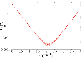
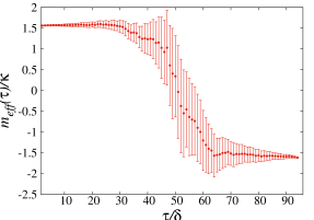
Figure 5: Example of $G_{-}(\tau)$ correlator (left panel) with momentum $|\vec{T}|(|k_{||}|,|k_{\bot,i}|)=\left(\frac{2\pi}{3},\frac{4\pi}{3\sqrt{3}}\right)$. The corresponding effective mass plot (in units of hopping parameter $\kappa$) is given underneath with $\Delta=2$ (right panel). Calculations were performed with $N_{L}=9$ and $N_{t}=96$.

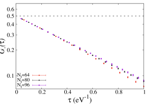
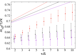
Figure 6: The $G_{-}(\tau)$ correlator (left panel) at the Dirac point for a (3,3) armchair with $N_{L}=$9 unit cells, using different numbers of timesteps as shown in the figure. Note that in this case $G_{+}(\tau)=G_{-}(\tau)$. The dashed line is the non-interacting result. The right panel shows the corresponding effective masses (points). Also shown in the right panel are the calculated correlators (lines) in the quenched approximation. To facilitate presentation, the quenched results have been shifted above the effective mass points such that their y-intercepts (at $\tau/\delta=0$) are .68.

We have also benchmarked our code to cases where analytic solutions are known, or where solutions can be obtained via direct numerical diagonalization, specifically the two- and four-site Hubbard models. We discuss these benchmark calculations in Appendix B.

VI.1 The Dirac K point

We now describe in detail our analysis for the Dirac K point. In the left panel of Fig. 6, we show the $G_{-}(\tau)$ correlator on a logarithmic scale at the Dirac point for different values of $N_{t}$. In the right panel of Fig. 6, we show the corresponding effective mass using $\Delta=2$. Also shown is the expected linear behavior of the effective mass for these calculations in the quenched approximation (lines), as discussed in Section V.3. Our dynamical calculations exhibit the same qualitative features as the quenched approximation. In particular, there is a clear linear behavior for the effective mass, particularly for smaller $N_{t}$. However, the slopes are not as steep as in the quenched approximation. Indeed, for $N_{t}=96$, a linear contribution is hardly discernible in the dynamical case for the shown range of time steps, but is nevertheless statistically significant.

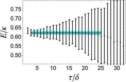
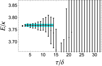
Figure 7: The extracted energy at the Dirac point (left panel, cyan band) for the $N_{L}=9$, $N_{t}=96$ calculation using the fitting procedure described in the text. The right panel shows extracted energy at the $\Gamma$ point. The effective mass points are given by the black data points and are shown for comparison. They were not used in the fitting procedure (see text). In both plots, the fitted Gaussian term has been subtracted from the effective mass points.

As we do not know the analytic form of the slope in the dynamical case, we perform simultaneous fits of both the leading exponential term (which provides the energy) and Gaussian term (which is responsible for the slope) directly to our correlators within a specific time window to extract our spectrum. We stress that we do not perform fits to the effective mass points (Eqn. (70)) themselves, but only to the correlator. In the left panel of Fig. 7 we show the extracted energy for the Dirac point determined by this fitting procedure. Note that the Gaussian contribution has been subtracted from the effective mass points in this figure. The agreement between the effective mass points and our fitted energy (cyan band) provides a consistency check on our fitting routines. The time window giving the optimal fit is given by the horizontal width of the band in the figure, whereas the the height provides the 1-$\sigma$ uncertainty, which in this case is the combination (in quadrature) of statistical and systematic errors. We estimate systematic errors by analyzing the distribution of fit results performed with varying time-window widths.

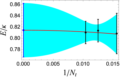
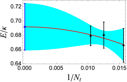
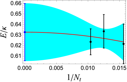
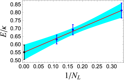
Figure 8: Continuum and inifinite-volume extrapolations of the Dirac point. The continuum-limit extrapolations for the $N_{L}=3$ (upper left), $N_{L}=6$ (upper right), and $N_{L}=9$ (bottom left) systems, using a scaling function quadratic in $\delta$. The continuum-limit results are used in an infinite-volume extrapolation (bottom right), assuming a linear dependence in $1/N_{L}$.

In Tabs. 3-5, we give the extracted energy at the Dirac point for each of our Monte Carlo calculations, as obtained from data with momentum $|\vec{T}|(|k_{||}|,|k_{\bot,i}|)=\left(\frac{2\pi}{3},\frac{2\pi}{\sqrt{3}}\right)$. For each value of $N_{L}$, we perform a continuum ($\delta\to 0$) extrapolation using the functional form $E(\delta)=E_{0}+C_{t}\delta^{2}$. The extrapolation is determined by multiple fits of the data, where each data point is sampled according to a normal distribution given by the combined statistical and systematic errors reported in Tabs. 3-5. This distribution of fits is then used to estimate the uncertainty of the extrapolation. The results in the continuum limit, and their associated uncertainties, are given in the last columns of Tabs. 3-5. In Fig. 8, we show this extrapolation for the Dirac point. As can be seen from Fig. 8, the data points at each value of $\delta$ are mutually consistent within uncertainties. This prevents us from determining with certainty that the discrete-time scaling is quadratic in $\delta$. Increased statistics, in addition to calculations at smaller values of $\delta$, would be needed.

Using the continuum-limit results at each $N_{L}$, we finally perform an infinite-volume, $N_{L}\rightarrow\infty$ (infinitely long tube) extrapolation. We find that our data extrapolates well with a simple linear dependence on $1/N_{L}$, and therefore we use the following functional form to perform our extrapolation: $E(N_{L})=E_{\infty}+C_{L}/N_{L}$. Quoted uncertainties of our infinite-volume extrapolation are determined in a similar fashion as our continuum-limit extrapolations. The extrapolation is shown in the bottom right panel of Fig. 8. We find that the energy at the Dirac point is $E_{K}/\kappa=.551(46)$. We note that the true volume dependence of our calculations may be something other than linear (see Assaad and Herbut (2013), for example, for a discussion of finite-volume scaling within low-dimension systems). However, our three points, and their associated uncertainties, are not sufficient to discern anything that deviates from linear dependence. Future studies, with larger values or $N_{L}$, should provide answers to this question.

VI.2 Spectrum of the (3,3) carbon nanotube

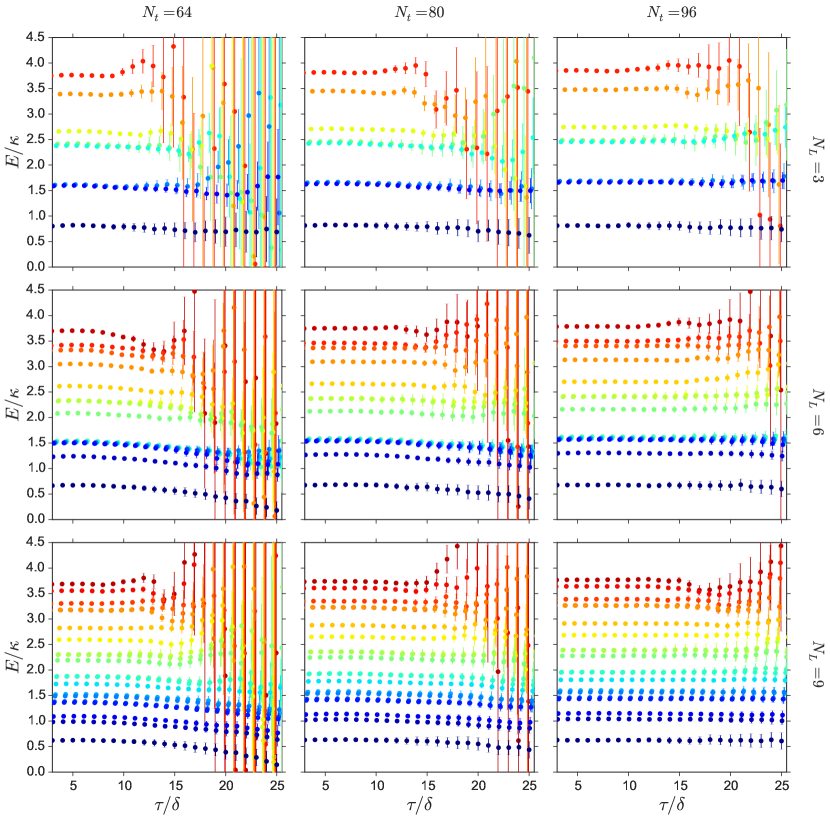
Figure 9: The effective masses from all accessible momenta, with Gaussian term subtracted. From top to bottom, the rows label $N_{L}=3$, 6, and 9 calculations, respectively. From left to right, the columns represent $N_{t}=64$, 80, and 96 calculations, respectively.

With our analysis formalism described in the preceding section, we now present the results of the remaining spectrum points for the (3,3) tube. In Fig. 9 we show the effective masses (with Gaussian term subtracted) for all accessible momenta for each of our calculations. Note that the $N_{L}=3$ case has less effective mass points than $N_{L}=6$, which in turn has less effective mass points than $N_{L}=9$. This is due to the fact that the number of accessible momenta increases as $N_{L}$ increases. In generating these figures, only the $G_{-}(\vec{k},\tau)$ electron correlators were analyzed since statistics for the $G_{+}(\vec{k},\tau)$ correlators were too poor for analysis. Also, correlators with degenerate energies were combined to increase statistics. A close-up of the effective mass plot for the $\Gamma$ point, as well as the fitted energy, is shown in the right panel of Fig. 7 for the $N_{L}=9$, $N_{t}=96$ case.

In tabs. 3-5 we list all the extracted energies for each $N_{L}$, $N_{t}$, and momentum point. The continuum-limit extrapolation is given in the last column of these tables. Figure 10 shows another example of this extrapolation but this time at the $\Gamma$ point. As opposed to the Dirac point, the data points at different $\delta$ are statistically distinct, but still not sufficient to discern linear or quadratic in $\delta$ scaling. To be consistent with the Dirac point analysis, we assume a quadratic scaling for the $\Gamma$ point as well as all other points on the dispersion. Again, future studies with smaller values of $\delta$ should tell whether such an assumption is valid.

In Fig. 11 we show all continuum-limit results for each $N_{L}$ system, compared to the non-interacting dispersion (dashed lines). As we only analyze the $G_{-}(\tau)$ correlators, and combine degenerate correlators when possible to increase statistics, we only show the upper-right portion of the dispersions in this figure (compare with Fig. 2).

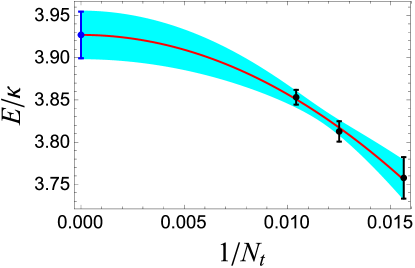
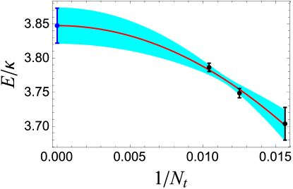
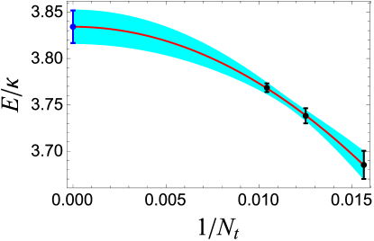
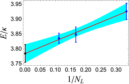
Figure 10: Continuum and inifinite-volume extrapolations of the $\Gamma$ point. The continuum-limit extrapolations for the $N_{L}=3$ (upper left), $N_{L}=6$ (upper right), and $N_{L}=9$ (bottom left) systems, using a scaling function quadratic in $\delta$. The continuum-limit results are used in an infinite-volume extrapolation (bottom right), assuming a linear dependence in $1/N_{L}$.

Table 3: Extracted energies for $N_{L}=3$ at different $N_{t}$ points. All energies are given in units of the hopping parameter $\kappa$. The first uncertainty is statistical, the second systematic. The last column gives the continuum-limit extrapolation assuming a $\delta^{2}$ scaling. Statistical and systematic errors were combined in quadrature to perform the extrapolation.

$|\vec{T}|\ (|k_{||}|,|k_{\bot,i}|)$	$E(N_{t}=64)$	$E(N_{t}=80)$	$E(N_{t}=96)$	$E(N_{t}=\infty)$
$\left(0,0\right)$	3.758(15)(19)	3.813(9)(8)	3.853(7)(5)	3.926(28)
$\left(0,\frac{2\pi}{3\sqrt{3}}\right)$	3.391(23)(19)	3.447(14)(19)	3.476(10)(4)	3.546(35)
$\left(0,\frac{4\pi}{3\sqrt{3}}\right)$	2.413(44)(36)	2.460(28)(11)	2.483(22)(6)	2.540(68)
$\left(0,\frac{2\pi}{\sqrt{3}}\right)$	1.614(13)(25)	1.655(8)(12)	1.688(6)(5)	1.744(31)
$\left(\frac{2\pi}{3},0\right)$	2.658(9)(17)	2.708(5)(12)	2.744(4)(3)	2.810(21)
$\left(\frac{2\pi}{3},\frac{2\pi}{3\sqrt{3}}\right)$	2.376(9)(19)	2.423(6)(16)	2.455(5)(2)	2.516(24)
$\left(\frac{2\pi}{3},\frac{4\pi}{3\sqrt{3}}\right)$	1.591(16)(22)	1.628(10)(11)	1.661(7)(3)	1.709(29)
$\left(\frac{2\pi}{3},\frac{2\pi}{\sqrt{3}}\right)$	0.808(25)(26)	0.814(18)(9)	0.810(11)(4)	0.813(47)

Table 4: Similar to Table 3, but for $N_{L}=6$.

$|\vec{T}|\ (|k_{||}|,|k_{\bot,i}|)$	$E(N_{t}=64)$	$E(N_{t}=80)$	$E(N_{t}=96)$	$E(N_{t}=\infty)$
$\left(0,0\right)$	3.704(9)(22)	3.749(6)(3)	3.786(5)(3)	3.848(26)
$\left(0,\frac{2\pi}{3\sqrt{3}}\right)$	3.322(16)(21)	3.368(15)(8)	3.403(9)(3)	3.464(32)
$\left(0,\frac{4\pi}{3\sqrt{3}}\right)$	2.330(32)(29)	2.371(29)(8)	2.418(15)(3)	2.477(53)
$\left(0,\frac{2\pi}{\sqrt{3}}\right)$	1.540(8)(18)	1.584(7)(8)	1.623(5)(5)	1.684(23)
$\left(\frac{\pi}{3},0\right)$	3.417(5)(15)	3.462(5)(6)	3.498(3)(1)	3.556(18)
$\left(\frac{\pi}{3},\frac{2\pi}{3\sqrt{3}}\right)$	3.047(10)(18)	3.094(9)(4)	3.132(5)(2)	3.195(23)
$\left(\frac{\pi}{3},\frac{4\pi}{3\sqrt{3}}\right)$	2.081(18)(21)	2.121(17)(7)	2.161(10)(2)	2.219(33)
$\left(\frac{\pi}{3},\frac{2\pi}{\sqrt{3}}\right)$	1.234(7)(19)	1.272(5)(9)	1.304(4)(5)	1.355(22)
$\left(\frac{2\pi}{3},0\right)$	2.617(6)(17)	2.664(4)(4)	2.702(3)(2)	2.766(18)
$\left(\frac{2\pi}{3},\frac{2\pi}{3\sqrt{3}}\right)$	2.325(7)(17)	2.373(6)(6)	2.408(4)(1)	2.471(20)
$\left(\frac{2\pi}{3},\frac{4\pi}{3\sqrt{3}}\right)$	1.513(12)(15)	1.556(9)(8)	1.588(6)(2)	1.644(22)
$\left(\frac{2\pi}{3},\frac{2\pi}{\sqrt{3}}\right)$	0.666(16)(17)	0.680(16)(9)	0.679(13)(3)	0.693(32)
$\left(\pi,0\right)$	1.499(7)(14)	1.540(7)(7)	1.572(4)(4)	1.627(18)
$\left(\pi,\frac{2\pi}{3\sqrt{3}}\right)$	1.518(6)(16)	1.560(5)(8)	1.591(3)(4)	1.647(19)
$\left(\pi,\frac{4\pi}{3\sqrt{3}}\right)$	1.518(6)(13)	1.561(5)(9)	1.590(3)(4)	1.647(18)
$\left(\pi,\frac{2\pi}{\sqrt{3}}\right)$	1.499(7)(18)	1.543(6)(11)	1.568(5)(5)	1.622(23)

Table 5: Similar to Table 3, but for $N_{L}=9$.

$|\vec{T}|\ (|k_{||}|,|k_{\bot,i}|)$	$E(N_{t}=64)$	$E(N_{t}=80)$	$E(N_{t}=96)$	$E(N_{t}=\infty)$
$\left(0,0\right)$	3.685(7)(13)	3.738(7)(5)	3.768(4)(2)	3.836(17)
$\left(0,\frac{2\pi}{3\sqrt{3}}\right)$	3.299(19)(11)	3.351(11)(3)	3.390(10)(2)	3.459(27)
$\left(0,\frac{4\pi}{3\sqrt{3}}\right)$	2.305(39)(52)	2.362(20)(7)	2.393(19)(4)	2.464(74)
$\left(0,\frac{2\pi}{\sqrt{3}}\right)$	1.520(7)(11)	1.576(7)(10)	1.598(4)(4)	1.663(17)
$\left(\frac{2\pi}{9},0\right)$	3.554(6)(10)	3.608(5)(3)	3.640(3)(3)	3.709(14)
$\left(\frac{2\pi}{9},\frac{2\pi}{3\sqrt{3}}\right)$	3.177(13)(9)	3.229(8)(3)	3.266(6)(1)	3.336(19)
$\left(\frac{2\pi}{9},\frac{4\pi}{3\sqrt{3}}\right)$	2.193(27)(11)	2.247(14)(5)	2.278(14)(3)	2.345(36)
$\left(\frac{2\pi}{9},\frac{2\pi}{\sqrt{3}}\right)$	1.382(5)(13)	1.436(5)(11)	1.458(3)(3)	1.522(17)
$\left(\frac{4\pi}{9},0\right)$	3.179(5)(10)	3.232(5)(5)	3.267(3)(3)	3.336(13)
$\left(\frac{4\pi}{9},\frac{2\pi}{3\sqrt{3}}\right)$	2.823(11)(7)	2.879(6)(6)	2.914(6)(2)	2.986(16)
$\left(\frac{4\pi}{9},\frac{4\pi}{3\sqrt{3}}\right)$	1.877(20)(9)	1.931(11)(7)	1.960(10)(3)	2.026(28)
$\left(\frac{4\pi}{9},\frac{2\pi}{\sqrt{3}}\right)$	0.987(6)(11)	1.028(6)(11)	1.038(4)(3)	1.083(17)
$\left(\frac{2\pi}{3},0\right)$	2.596(5)(9)	2.650(4)(6)	2.684(3)(2)	2.753(13)
$\left(\frac{2\pi}{3},\frac{2\pi}{3\sqrt{3}}\right)$	2.299(8)(10)	2.357(5)(7)	2.390(4)(1)	2.461(14)
$\left(\frac{2\pi}{3},\frac{4\pi}{3\sqrt{3}}\right)$	1.490(14)(12)	1.541(8)(8)	1.565(7)(2)	1.628(23)
$\left(\frac{2\pi}{3},\frac{2\pi}{\sqrt{3}}\right)$	0.622(16)(10)	0.634(15)(5)	0.624(7)(2)	0.631(23)
$\left(\frac{8\pi}{9},0\right)$	1.871(5)(11)	1.926(4)(8)	1.956(2)(3)	2.025(15)
$\left(\frac{8\pi}{9},\frac{2\pi}{3\sqrt{3}}\right)$	1.729(5)(9)	1.781(3)(7)	1.809(2)(1)	1.874(12)
$\left(\frac{8\pi}{9},\frac{4\pi}{3\sqrt{3}}\right)$	1.362(6)(10)	1.412(4)(9)	1.433(3)(1)	1.493(13)
$\left(\frac{8\pi}{9},\frac{2\pi}{\sqrt{3}}\right)$	1.093(6)(11)	1.135(5)(10)	1.151(3)(3)	1.201(15)

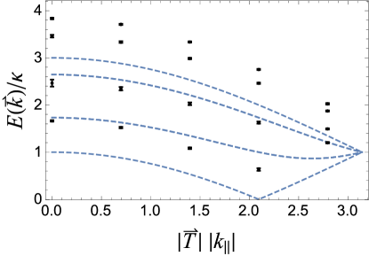
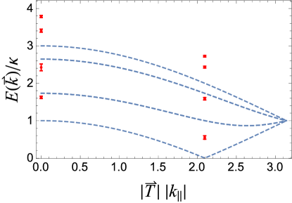
Figure 11: Continuum-limit extrapolated spectrum of quasi-electron (black points) compared to non-interacting dispersion relation (dashed line) for the (3,3) tube with $N_{L}=3$ (upper left), 6 (upper right), and 9 (bottom left) calculations. The bottom right panel shows the infinite-volume extrapolation of points common to all $N_{L}=3$, 6, and 9 systems, given by the last column in Table 6.

To perform an infinite-volume extrapolation, we must use momenta which are common in all $N_{L}=3$, 6, and 9 cases, which as can be seen from Fig. 11 occurs for points that have $|\vec{T}||k_{||}|=$ 0 and $2\pi/3$. We tabulate these points in Table 6.

Table 6: Infinite-volume extrapolations of momentum points common to $N_{L}=3$, 6, and 9 systems (last column) and their corresponding momenta (first column), and the points used to perform the extrapolation (middle columns). Energies are shown in units of $\kappa$. The functional form of the extrapolation is linear in $1/N_{L}$.

$|\vec{T}|\ (|k_{||}|,|k_{\bot,i}|)$	$E(N_{L}=3)$	$E(N_{L}=6)$	$E(N_{L}=9)$	$E(N_{L}=\infty)$
$\left(0,0\right)$	3.926(28)	3.848(26)	3.836(17)	3.784(29)
$\left(0,\frac{2\pi}{3\sqrt{3}}\right)$	3.546(35)	3.464(32)	3.459(27)	3.406(41)
$\left(0,\frac{4\pi}{3\sqrt{3}}\right)$	2.540(68)	2.477(53)	2.464(74)	2.424(91)
$\left(0,\frac{2\pi}{\sqrt{3}}\right)$	1.744(31)	1.684(23)	1.663(17)	1.623(31)
$\left(\frac{2\pi}{3},0\right)$	2.810(21)	2.766(18)	2.753(13)	2.723(21)
$\left(\frac{2\pi}{3},\frac{2\pi}{3\sqrt{3}}\right)$	2.516(24)	2.471(20)	2.461(14)	2.433(25)
$\left(\frac{2\pi}{3},\frac{4\pi}{3\sqrt{3}}\right)$	1.709(29)	1.644(22)	1.628(23)	1.586(32)
$\left(\frac{2\pi}{3},\frac{2\pi}{\sqrt{3}}\right)$	0.813(47)	0.693(32)	0.632(28)	0.551(46)

In the bottom right panel of Fig. 11 we plot these points along with the non-interacting dispersion. The effects of strongly-correlated electrons is clearly seen in the calculated spectrum of this system, and in general lifts all points above their non-interacting values.

VII Conclusions

We have demonstrated how lattice Monte Carlo methods can be applied to carbon nanotubes. We have derived the path-integral formalism for such systems, based on previous work for a planar hexagonal lattice, with appropriate (periodic) boundary conditions that depend on the nanotube chirality $(n,m)$. In so doing, we emphasized differences of our method with previous lattice Monte Carlo calculations of graphene, as well as with lattice QCD. We proceeded to benchmark our method for the (3,3) armchair nanotube, using the screened Coulomb interaction of Ref. Smith and von Smekal (2014) which incorporates the values of $U_{00}$ through $U_{03}$ found by Ref. Wehling et al. (2011). Apart from the requirement that the potential matrix $V_{xy}$ be positive definite, we stress that our formalism is not dependent on any particular parametrization of the electron-electron interaction.

As opposed to previous lattice Monte Carlo simulations, we extracted single quasi-particle energies by direct analysis of the momentum-projected one-body correlators, a method commonly used by LQCD calculations. This allowed us to not only extract the spectrum at the Dirac point, but at all allowed momentum modes. As the nanotube systems studied were relatively small, we were able to perform calculations at multiple time steps $N_{t}$ and multiple tube lengths $N_{L}$. The former allowed us to perform a continuum limit extrapolation, and the latter allowed us to consider nanotubes of infinite length. In all cases, we found that the non-interacting spectrum is strongly modified by electron-electron correlation effects, in general raising the energies at all points in the Brillouin zone above their non-interacting (tight-binding) values. In particular, our result for the energy of the Dirac point in the (3,3) nanotube was found to be $E_{K}/\kappa=.551(46)$, consistent with a substantial interaction-induced energy gap in this (nominally) metallic nanotube.

Our extrapolations in the temporal and spatial dimensions used simple scaling functions in $\delta^{2}$ and $1/N_{L}$. Though we have performed multiple Monte Carlo calculations for different $\delta$ and $N_{L}$, our preliminary results are not yet sufficient to exclude other possible power-law scalings. Systematic errors from other possible scalings have thus not been included in our analysis, although we note that future studies using a larger set of $\delta$ and $N_{L}$ values can address this issue. We also found that the small physical dimensions of our nanotubes, coupled with the long-range nature of the Coulomb interaction, induced a Gaussian term in our correlators, which we attributed to the zero-mode contributions of our auxiliary field. To account for this effect in our analysis of the large-time behavior of our correlators, we performed simultaneous fits of both Gaussian and (leading) exponential terms.

A possible application of our method would be to consider the energy gap at the Dirac point as a function of nanotube radius, for which considerable experimental data is available. Such calculations would allow for a direct test of different models for the electron-electron interaction, which in turn could provide additional input to the problem of a possible Mott insulating state in suspended graphene. Also, while we have so far only considered the single-quasiparticle dispersion relation, our formalism can easily be extended to the spectrum of multi-particle states. For example, the interacting $J=0$ electron-hole system can be represented by the “interpolating operator” $O^{\dagger}(x,y)\equiv 1/\!\sqrt{2}\,[a_{-}^{\dagger}(x)b_{-}^{\dagger}(y)-b_{-}^{\dagger}(x)a_{-}^{\dagger}(y)]$, where the operators $a^{\dagger}_{\pm}$ and $b^{\dagger}_{\pm}$ are defined in Eqn. (63). The spectrum of such a system could be ascertained by analyzing the temporal behavior of the two-particle correlator $\left\langle O(x^{\prime},y^{\prime})O^{\dagger}(x,y)\right\rangle$. In light of the results found in Matsunaga et al. (2011), such studies would be very interesting.

Our relatively large uncertainties can be traced back to the non-trivial contribution of zero-modes to our correlators and the fact that our system is physically very small. Both contributions can be alleviated by increasing the volume (length) of our system. As in LQCD, we anticipate a suppression of uncertainties that scale as $1/V^{3/2}$, where $V$ is the volume of the system Luscher (2010). This would correspond to uncertainties that scale as $1/N_{L}^{1/2}$ for our system. Such suppression is already evident when comparing the uncertainties between our $N_{L}$=3, 6, and 9 calculations (Tables 3-5). However, the dimensions of such calculations would scale linearly in $N_{L}$. We expect reduced uncertainties with larger diameter tube calculations as well. The dimension of a (14,14) tube calculation with $N_{L}=9$, for example, is $\simeq$ 20 times larger than the (3,3) system with $N_{L}=9$ and same number of time steps. Such a calculation would require resources beyond what we have committed to this paper, i.e. desktop workstation (we are currently modifying our codes to run on larger computer clusters), and would be ideally suited for GPUs Wendt et al. (2011); Brower et al. (2011); Smith and von Smekal (2014).

In conclusion, we emphasize that our Monte Carlo method is completely general and can be applied to other carbon nanostructures, such as graphene single- and multi-layers, multi-wall nanotubes and carbon nano-ribbons. The most significant restriction of our method is the requirement of a positive definite probability measure, the availability of which has to be assessed on a case-by-case basis. In addition to periodic boundary conditions, our method also allows for arbitrary boundary conditions (such as open or twisted boundary conditions). For instance, the latter choice could prove useful in studies of carbon nanotubes in an external magnetic field.

Appendix A Zero-mode contributions to the path integral

We begin with the continuum limit (in time) expression for the expectation value of our fermion correlator in the quenched approximation (i.e. setting $\det(M[\Phi]M^{\dagger}[\Phi])=1$ in eq. (21)),

$$\langle M^{-1}(\vec{k}_{\alpha},\tau)\rangle=\frac{1}{Z}\int\mathcal{D}\tilde{\Phi}\ e^{-S[\Phi]}\frac{1}{\beta}\sum_{n=-\infty}^{\infty}e^{-i\omega_{n}\tau}M^{-1}(\vec{k}_{\alpha},\omega_{n};\Phi_{x_{0}}(t_{0}))\ ,$$ (71)

where

$$S[\Phi] = \frac{1}{2}\int_{0}^{\beta}dt\sum_{x,y\in\{X\}}\Phi^{T}_{x}(t)[V^{-1}]_{x,y}\Phi_{y}(t)$$ (72)

$$\omega_{n} = \pi(2n+1)/\beta\ ,$$ (73)

and

$$M^{-1}(\vec{k}_{\alpha},\omega_{n};\Phi_{x_{0}}(t_{0}))=\ \left((i\omega_{n}-\omega_{+})(i\omega_{n}-\omega_{-})\right)^{-1}m(i\omega_{n},\vec{k}_{\alpha},\Phi_{x_{0}}(t_{0}))\ ,$$ (74)

where $m(i\omega_{n},\vec{k}_{\alpha},\Phi_{x_{0}}(t_{0}))$ is the following 2$\times$2 matrix

$$m(i\omega_{n},\vec{k}_{\alpha},\Phi_{x_{0}}(t_{0}))=\begin{pmatrix}-(i\omega_{n}+i\phi^{B}_{x_{0}}(t_{0})+U_{00}/2)&\kappa f(\vec{k}_{\alpha})\\ \kappa f^{*}(\vec{k}_{\alpha})&-(i\omega_{n}+i\phi^{A}_{x_{0}}(t_{0})+U_{00}/2)\end{pmatrix}\ .$$ (75)

The matrix $m(i\omega_{n},\vec{k}_{\alpha},\Phi_{x_{0}}(t_{0})$ contains no poles. The frequencies $\omega_{\pm}$ are

$$\omega_{\pm} = -i\frac{(\phi^{A}_{x_{0}}(t_{0})+\phi^{B}_{x_{0}}(t_{0}))}{2}-\frac{U_{00}}{2}\pm i\sqrt{\left(\frac{\phi^{A}_{x_{0}}(t_{0})-\phi^{B}_{x_{0}}(t_{0})}{2}\right)^{2}+|\kappa f(\vec{k}_{\alpha})|^{2}}$$ (76)

$$\equiv -i\frac{(\phi^{A}_{x_{0}}(t_{0})+\phi^{B}_{x_{0}}(t_{0}))}{2}-\frac{U_{00}}{2}\pm i\Delta\omega\ .$$ (77)

We first concentrate on the frequency sum in Eqn. (71), which using Eqns. (75)-(77) can be written as

$$\frac{1}{\beta}\sum_{n=-\infty}^{\infty}\frac{e^{-i\omega_{n}\tau}}{(i\omega_{n}-\omega_{+})(i\omega_{n}-\omega_{-})}m(i\omega_{n},\vec{k}_{\alpha},\Phi_{x_{0}}(t_{0}))\ .$$ (78)

Assuming that $0\leq\tau\leq\beta$, one can use the Matsubara weighting function $h(\omega)=(1+\exp(-\beta\omega))^{-1}$ and standard finite-temperature integration techniques Abrikosov et al. (1975); Mattuck (2012) to show that the sum in Eqn. (78) is equal to

$$\frac{1}{\beta}\frac{1}{(\omega_{-}-\omega_{+})}\left(e^{-\omega_{+}\tau}m(\omega_{+},\vec{k}_{\alpha},\Phi_{x_{0}}(t_{0}))h(\omega_{+})-e^{-\omega_{-}\tau}m(\omega_{-},\vec{k}_{\alpha},\Phi_{x_{0}}(t_{0}))h(\omega_{-})\right)\\ =e^{i(\phi^{A}_{x_{0}}(t_{0})+\phi^{B}_{x_{0}}(t_{0}))\frac{\tau}{2}}\frac{1}{\beta}\frac{e^{U_{00}\frac{\tau}{2}}}{(\omega_{-}-\omega_{+})}\times\\ \left(e^{-\Delta\omega\tau}m(\omega_{+},\vec{k}_{\alpha},\Phi_{x_{0}}(t_{0}))h(\omega_{+})-e^{\Delta\omega\tau}m(\omega_{-},\vec{k}_{\alpha},\Phi_{x_{0}}(t_{0}))h(\omega_{-})\right)\ .$$ (79)

We concentrate on the small time dependence, $\tau\ll\beta$, of our expression and perform a small temperature, large $\beta$ expansion of the Matsubara regulator,

$$h(\omega_{\pm})=1-e^{-\beta\omega_{\pm}}+e^{-2\beta\omega_{\pm}}+\ldots$$

To leading order in this expansion, we have

$$\frac{1}{\beta}\frac{1}{(\omega_{-}-\omega_{+})}\left(e^{-\omega_{+}\tau}m(\omega_{+},\vec{k}_{\alpha},\Phi_{x_{0}}(t_{0}))-e^{-\omega_{-}\tau}m(\omega_{-},\vec{k}_{\alpha},\Phi_{x_{0}}(t_{0}))\right)+\mathcal{O}(e^{-\beta\omega_{\pm}})\\ =e^{i(\phi^{A}_{x_{0}}(t_{0})+\phi^{B}_{x_{0}}(t_{0}))\frac{\tau}{2}}\frac{1}{\beta}\frac{e^{U_{00}\frac{\tau}{2}}}{(\omega_{-}-\omega_{+})}\left(e^{-\Delta\omega\tau}m(\omega_{+},\vec{k}_{\alpha},\Phi_{x_{0}}(t_{0}))-e^{\Delta\omega\tau}m(\omega_{-},\vec{k}_{\alpha},\Phi_{x_{0}}(t_{0}))\right)\\ \equiv e^{i(\phi^{A}_{x_{0}}(t_{0})+\phi^{B}_{x_{0}}(t_{0}))\frac{\tau}{2}}F\left(\frac{\phi^{A}_{x_{0}}(t_{0})-\phi^{B}_{x_{0}}(t_{0})}{2},\tau\right)$$ (80)

where the function $F$ can be determined by comparing the second and third lines of the equation above. The argument structure of $F$ is written in such a manner as to stress the fact that its depencence on the auxiliary fields is through the difference $\phi^{A}_{x_{0}}(t_{0})-\phi^{B}_{x_{0}}(t_{0})$, which can be easily verified by analyzing Eqns. (75)-(77).

We now expand our auxiliary fields in momentum-frequency space,

$$\phi^{A,B}_{x_{0}}(\tau_{0}) = \frac{1}{\beta}\sum_{n=-\infty}^{\infty}e^{-i\omega_{n}\tau_{0}}\frac{1}{N}\sum_{k_{\alpha}\in\{K\}}e^{-i\vec{k}_{\alpha}\cdot\vec{x}_{0}}\hat{\phi}^{A,B}_{k_{\alpha},\omega_{n}}$$ (81)

$$= \frac{1}{\beta N}\hat{\phi}^{A,B}_{0}+\frac{1}{\beta N}\sum_{\{n,k_{\alpha}\}\neq\{0,0\}}e^{-i\omega_{n}\tau_{0}}e^{-i\vec{k}_{\alpha}\cdot\vec{x}_{0}}\hat{\phi}^{A,B}_{k_{\alpha},\omega_{n}}\ ,$$ (82)

where in the second line we explicitly separate the zero-mode contribution. Note that the frequency sum is over bosonic frequencies, $\omega_{n}=2\pi n/\beta$, and $N$ is the number of hexagons in our calculation. Further, it is convenient to define the fields $\hat{\phi}^{\pm}_{0}$ through the following linear combinations of the fields in momentum-frequency space,

$$\frac{\phi^{A}_{x_{0}}(\tau_{0})\pm\phi^{B}_{x_{0}}(\tau_{0})}{2} = \frac{1}{\beta N}\frac{\hat{\phi}^{A}_{0}\pm\hat{\phi}^{B}_{0}}{2}+\frac{1}{\beta N}\sum_{\{n,k_{\alpha}\}\neq\{0,0\}}e^{-i\omega_{n}\tau_{0}}e^{-i\vec{k}_{\alpha}\cdot\vec{x}_{0}}\frac{(\hat{\phi}^{A}_{k_{\alpha},\omega_{n}}\pm\hat{\phi}^{B}_{k_{\alpha},\omega_{n}})}{2}$$ (83)

$$\equiv \frac{1}{\beta N}\hat{\phi}^{\pm}_{0}+\Delta^{\pm}[\Phi_{k_{\alpha},\omega_{n}}]\ ,$$ (84)

where $\Delta^{\pm}[\Phi_{k_{\alpha},\omega_{n}}]$ contains sums over terms that have non-zero momentum or frequency modes.

The action in Eqn. (73) can be cast in momentum-frequency space,

$$S[\Phi] = \frac{1}{2}\frac{1}{\beta N}\sum_{n,k_{\alpha}}\hat{\Phi}^{T}_{k_{\alpha},\omega_{n}}[\hat{v}^{-1}]_{k_{\alpha}}\hat{\Phi}_{k_{\alpha},\omega_{n}}$$ (85)

$$= \frac{1}{2}\frac{1}{\beta N}\hat{\Phi}^{T}_{0}[\hat{v}^{-1}]_{0}\hat{\Phi}_{0}+\frac{1}{2}\frac{1}{\beta N}\sum_{\{n,k_{\alpha}\}\neq\{0,0\}}\hat{\Phi}^{T}_{k_{\alpha},\omega_{n}}[\hat{v}^{-1}]_{k_{\alpha}}\hat{\Phi}_{k_{\alpha},\omega_{n}}$$ (86)

$$\equiv \frac{1}{2}\frac{1}{\beta N}\hat{\Phi}^{T}_{0}[\hat{v}^{-1}]_{0}\hat{\Phi}_{0}+S[\hat{\Phi}_{k,\omega}]\ ,$$ (87)

where $\hat{v}_{k_{\alpha}}$ is the discrete fourier transform of the screened Coulomb potential and we have again separated out the zero-mode contribution and defined the remainder as $S[\hat{\Phi}_{k,\omega}]$. In terms of $\hat{\phi}^{A,B}_{0}$ we have that

$$\frac{1}{2}\frac{1}{\beta N}\hat{\Phi}^{T}_{0}[\hat{v}^{-1}]_{0}\hat{\Phi}_{0} = \frac{1}{2}\frac{1}{\beta N}\frac{1}{(\hat{v}^{AA}_{0})^{2}-(\hat{v}^{AB}_{0})^{2}}\left(\hat{v}^{AA}_{0}[(\hat{\phi}^{A}_{0})^{2}+(\hat{\phi}^{B}_{0})^{2}]-2\hat{v}^{AB}_{0}\hat{\phi}^{A}_{0}\hat{\phi}^{B}_{0}\right)$$

$$= \frac{1}{\beta N}\frac{1}{(\hat{v}^{AA}_{0})^{2}-(\hat{v}^{AB}_{0})^{2}}\left((\hat{\phi}^{+}_{0})^{2}(\hat{v}^{AA}_{0}-\hat{v}^{AB}_{0})+(\hat{\phi}^{-}_{0})^{2}(\hat{v}^{AA}_{0}+\hat{v}^{AB}_{0})\right)$$

$$\equiv \frac{1}{\beta N}\frac{(\hat{v}^{AA}_{0}-\hat{v}^{AB}_{0})}{(\hat{v}^{AA}_{0})^{2}-(\hat{v}^{AB}_{0})^{2}}(\hat{\phi}^{+}_{0})^{2}+S[\hat{\phi}^{-}_{0}]\ ,$$

where

$$\hat{v}^{AA}_{0} = \sum_{x\in\{X\}}V(|\vec{x}|)$$ (89)

$$\hat{v}^{AB}_{0} = \sum_{x\in\{X\}}V(|\vec{x}+\vec{a}|)\ ,$$ (90)

and $\vec{a}$ is the basis unit vector. Finally we factor out the zero mode measures in the integration measure,

$$\mathcal{D}\Phi=d\hat{\phi}^{A}_{0}d\hat{\phi}^{B}_{0}\mathcal{D}\Phi_{(k_{\alpha},\omega)\neq(0,0)}=d\hat{\phi}^{+}_{0}d\hat{\phi}^{-}_{0}\mathcal{D}\Phi_{(k_{\alpha},\omega)\neq(0,0)}\ .$$ (91)

The Jacobian from the change of variables in the last expression is unity. Combining Eqns. (80), (84), (87), (A), and (91), one gets

$$\int d\hat{\phi}^{+}_{0}\exp\left\{-\frac{1}{\beta N}\left(\frac{(\hat{v}^{AA}_{0}-\hat{v}^{AB}_{0})}{(\hat{v}^{AA}_{0})^{2}-(\hat{v}^{AB}_{0})^{2}}(\hat{\phi}^{+}_{0})^{2}-i\hat{\phi}^{+}_{0}\tau\right)\right\}\times\\ \int d\hat{\phi}^{-}_{0}\mathcal{D}\Phi_{(k_{\alpha},\omega)\neq(0,0)}e^{-S[\hat{\phi}^{-}_{0}]-S[\hat{\Phi}_{k_{\alpha},\omega}]+i\Delta^{+}[\Phi_{k_{\alpha},\omega}]\tau}F\left(\hat{\phi}^{-}_{0}+\Delta^{-}[\Phi_{k_{\alpha},\omega}],\tau\right)\ .$$ (92)

We can now perform the integral over $\hat{\phi}^{+}_{0}$ explicitly. Up to an irrelvant multiplicative factor, the result is

$$\exp\left\{-\frac{(\hat{v}^{AA}_{0}+\hat{v}^{AB}_{0})}{4\beta N}\tau^{2}\right\}\\ \int d\hat{\phi}^{-}_{0}\mathcal{D}\Phi_{(k_{\alpha},\omega)\neq(0,0)}e^{-S[\hat{\phi}^{-}_{0}]-S[\hat{\Phi}_{k_{\alpha},\omega}]+i\Delta^{+}[\Phi_{k_{\alpha},\omega}]\tau}F\left(\hat{\phi}^{-}_{0}+\Delta^{-}[\Phi_{k_{\alpha},\omega}],\tau\right)\ ,$$ (93)

which shows the Gaussian dependence in $\tau$. The remaining functional integrals over $\hat{\phi}^{-}_{0}$ and $\mathcal{D}\Phi_{(k_{\alpha},\omega)\neq(0,0)}$ produce exponential depencence in the spectrum $E_{i}(\vec{k}_{\alpha})$ of the system. Thus for low temperatures, small time regime, and quenched approximation, our correlator behaves as

$$\langle M^{-1}(\vec{k}_{\alpha},\tau)\rangle\sim\exp\left\{-\frac{(\hat{v}^{AA}_{0}+\hat{v}^{AB}_{0})}{4\beta N}\tau^{2}\right\}\sum_{i}A_{i}e^{-E_{i}(\vec{k}_{\alpha})\tau}\ .$$ (94)

Appendix B Benchmark calculations of the 2-site and 4-site Hubbard model

We provide details of our benchmark calculations of correlators calculated with our lattice code compared to analytic calculations of the 2- and 4-site Hubbard model. As the Hubbard model has onsite interactions only (i.e. no long-range interaction) we do not have zero-mode induced Gaussian dependence in our correlators. The 4-site model has two momentum modes that allow us to test our momentum projection routines.

B.1 2-site Hubbard model

The simplest case that one can consider that includes interactions is the 2-site Hubbard model. The Hamiltonian for the Hubbard model at half-filling is

$$\hat{H}=-\kappa\sum_{\langle i,j\rangle}c^{{\dagger}}_{i,\sigma}c_{j,\sigma}+U_{00}\sum_{i}n_{i,\uparrow}n_{i,\downarrow}-\frac{U_{00}}{2}\sum_{i}\left(n_{i,\uparrow}+n_{i,\downarrow}\right)+\mbox{const.}\ ,$$ (95)

where $\langle i,j\rangle$ denotes nearest neighbor summation, $c^{{\dagger}}_{i,\sigma}$ ($c_{i,\sigma}$) is the creation (annihilation) operator for an electron of spin $\sigma$ at site $i$, $n_{i,\sigma}=c^{{\dagger}}_{i,\sigma}c_{i,\sigma}$ is the number operator for spin $\sigma$ at site $i$, and $U_{00}$ is the onsite repulsive interaction parameter. We note that the relevant dimensionless parameter in this model is simply the ratio $\lambda=U_{00}/\kappa$.

The eigenvalues of the system can be obtained by direct diagonalization, and the single-electron correlation function can be obtained using the expression

$$G_{ij}^{\sigma\sigma^{\prime}}(\tau)\equiv\langle c_{i,\sigma}(\tau)c^{{\dagger}}_{j,\sigma^{\prime}}(0)\rangle=\frac{1}{\mathcal{Z}}\sum_{i}\langle i|c_{i,\sigma}(\tau)c^{{\dagger}}_{j,\sigma^{\prime}}(0)|i\rangle e^{-\beta E_{i}}\ ,$$ (96)

where the sum is over eigenstates $|i\rangle$ of the system, $E_{i}$ is the eigenvalue for state $|i\rangle$, and

$$\mathcal{Z}=\sum_{i}e^{-\beta E_{i}}\ .$$

For a given $\beta$, $U$, and $\kappa$, we perform our lattice calculations and compare our calculated correlators with those derived analytically. In Fig. 12 we compare our lattice results with analytic results for the case when $U/\kappa=2$. Details of lattice calculation are given in the caption.

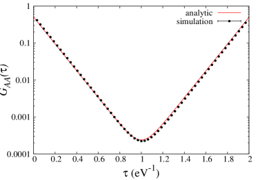
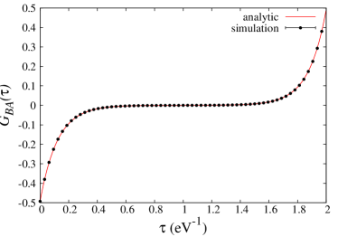
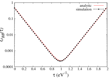
Figure 12: The matrix of correlators $G_{ij}(\tau)$ for 2-site Hubbard model with $\beta=2$ eV^-1 and $\kappa=2.7$ eV, and $U/\kappa=2$. The solid lines are the analytical results. The points are from a full lattice calculation with $N_{t}=64$ timesteps. Errorbars, obtained via boostrap, are too small to be visible.

The relevant correlators to extract energies are given by

$$G_{\pm}(\tau)\equiv\frac{1}{2}\left[G_{AA}(\tau)+G_{BB}(\tau)\pm\left(G_{AB}(\tau)+G_{BA}(\tau)\right)\right]\ .$$ (97)

Figure 13 shows comparison of lattice results using $N_{t}=64$ and $N_{t}=128$ compared with analytic results. Clear convergence with the analytic results is seen, particularly for the $G_{+}(\tau)$ correlator.

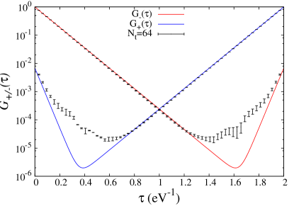
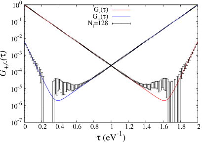
Figure 13: $G_{\pm}(\tau)$ correlators for 2-site Hubbard model with $\beta=2$ eV^-1 and $\kappa=2.7$ eV, and $U/\kappa=2$. The solid lines are the analytical results. Left (right) plot has $N_{t}=64\ (128)$ timesteps.

In Fig. 14 we show results for $G_{\pm}(\tau)$ for the case of $\beta=3$ eV^-1, $U/\kappa=4$, and $N_{t}=96$.

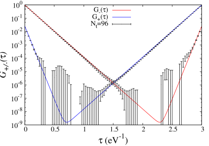
Figure 14: Comparison of numerical calculation of $G_{\pm}(\tau)$ with analytic result for $\beta=3$ eV^-1, $\kappa=2.7$ eV, $U/\kappa=4$, and $N_{t}=96$ timesteps. The solid line is the analytical result.

B.2 4-site Hubbard model

The 4-site Hubbard model is equivalent to the (1$\times$2) graphene lattice. There are two unit cells in this case, giving 4 ion positions in total. The Hamiltonian is the same as in Eqn. (95), however construction of the correlators is a little trickier since there are now two allowed momenta within the first BZ,

$$\vec{k}_{1}=(0,0)\quad,\quad\vec{k}_{2}=\left(\frac{\pi}{3a},-\frac{\pi}{\sqrt{3}a}\right)\ ,$$

Momentum projection on $G_{\pm}$ is given by

$$G_{\pm}(\vec{k}_{i},;\tau)=\frac{1}{4}\frac{1}{\mathcal{Z}}\times\\ \sum_{l,m=1}^{2}e^{i\vec{k}_{i}\cdot(\vec{x}_{l}-\vec{x}_{m})}\left[\langle c_{l}^{A}(\tau)c_{m}^{A{\dagger}}(0)\rangle+\langle c_{l}^{B}(\tau)c_{m}^{B{\dagger}}(0)\rangle\pm\left(\langle c_{l}^{A}(\tau)c_{m}^{B{\dagger}}(0)\rangle+\langle c_{l}^{B}(\tau)c_{m}^{A{\dagger}}(0)\rangle\right)\right]$$ (98)

where the sum is over the unit cells (not ion sites). In figs. 15 and  16 we show calculations compared to exact results (determined via diagonalization) for the different momentum projections, using $U_{00}=9.3$ eV and $\beta=6.4$ eV^-1. Calculations were done with $N_{t}$=128 and 256, and shows definitive convergence. Also shown are the non-interacting (NI) solutions.

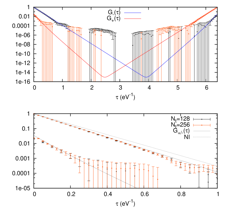
Figure 15: 4-site Hubbard calculation of $\vec{k}_{1}$ momentum correlators with $U_{00}=9.3$ eV and $\beta=6.4$ eV^-1. Bottom plot is a close up and shows the non-interacting results (dashed line).

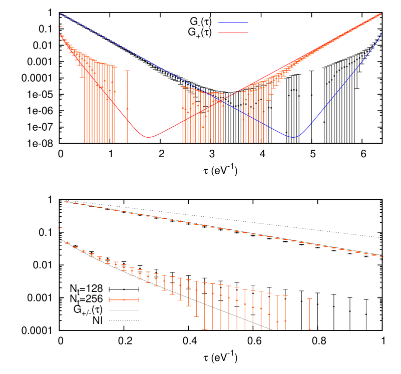
Figure 16: 4-site Hubbard calculation of $\vec{k}_{2}$ momentum correlators with $U_{00}=9.3$ eV and $\beta=6.4$ eV^-1. Bottom plot is a close up and shows the non-interacting results (dashed line).

In addition to onsite interactions, we have also benchmarked our codes to 2- and 4-site systems with onsite, nearest-neighbor, and next-to-nearest neighbor interactions. Though we do not show results of these studies here, we find our code gives equally good agreement with analytic and direct diagonalization methods. We note that for systems that have only onsite $U_{00}$ and nearest neighbor $U_{01}$ interactions, our Monte Carlo code fails due to instability of the Hubbard transformation.

References

- Deshpande et al. (2010) V. V. Deshpande, M. Bockrath, L. I. Glazman, and A. Yacoby, Nature 464, 209 (2010).
- Charlier et al. (2007) J.-C. Charlier, X. Blase, and S. Roche, Rev. Mod. Phys. 79, 677 (2007).
- Balents and Fisher (1997) L. Balents and M. P. A. Fisher, Phys. Rev. B 55, R11973 (1997).
- Chen et al. (2008) W. Chen, A. V. Andreev, A. M. Tsvelik, and Dror Orgad, Phys. Rev. Lett. 101, 246802 (2008).
- Novoselov et al. (2004) K. S. Novoselov, A. K. Geim, S. V. Morozov, D. Jiang, Y. Zhang, S. V. Dubonos, I. V. Grigorieva, and A. A. Firsov, Science 306, 666 (2004), http://www.sciencemag.org/content/306/5696/666.full.pdf .
- Novoselov et al. (2005a) K. S. Novoselov, D. Jiang, F. Schedin, T. J. Booth, V. V. Khotkevich, S. V. Morozov, and A. K. Geim, Proceedings of the National Academy of Sciences of the United States of America 102, 10451 (2005a), http://www.pnas.org/content/102/30/10451.full.pdf .
- Geim and Novoselov (2007) A. K. Geim and K. S. Novoselov, Nat Mater 6, 183 (2007).
- Castro Neto et al. (2009) A. H. Castro Neto, F. Guinea, N. M. R. Peres, K. S. Novoselov, and A. K. Geim, Rev. Mod. Phys. 81, 109 (2009).
- Novoselov et al. (2005b) K. S. Novoselov, A. K. Geim, S. V. Morozov, D. Jiang, M. I. Katsnelson, I. V. Grigorieva, S. V. Dubonos, and A. A. Firsov, Nature 438, 197 (2005b).
- Zhang et al. (2005) Y. Zhang, Y.-W. Tan, H. L. Stormer, and P. Kim, Nature 438, 201 (2005).
- Kane et al. (1997) C. Kane, L. Balents, and M. P. A. Fisher, Phys. Rev. Lett. 79, 5086 (1997).
- Bockrath et al. (1999) M. Bockrath, D. H. Cobden, J. Lu, A. G. Rinzler, R. E. Smalley, L. Balents, and P. L. McEuen, Nature 397, 598 (1999).
- Khveshchenko and Leal (2004) D. Khveshchenko and H. Leal, Nuclear Physics B 687, 323 (2004).
- Gamayun et al. (2010) O. V. Gamayun, E. V. Gorbar, and V. P. Gusynin, Phys. Rev. B 81, 075429 (2010).
- Odintsov and Yoshioka (1999) A. A. Odintsov and H. Yoshioka, Phys. Rev. B 59, R10457 (1999).
- Kotov et al. (2012) V. N. Kotov, B. Uchoa, V. M. Pereira, F. Guinea, and A. H. Castro Neto, Rev. Mod. Phys. 84, 1067 (2012).
- Herbut (2006) I. F. Herbut, Phys. Rev. Lett. 97, 146401 (2006).
- Throckmorton and Vafek (2012) R. E. Throckmorton and O. Vafek, Phys. Rev. B 86, 115447 (2012).
- Levitov and Tsvelik (2003) L. S. Levitov and A. M. Tsvelik, Phys. Rev. Lett. 90, 016401 (2003).
- Zhao and Mazumdar (2004) H. Zhao and S. Mazumdar, Phys. Rev. Lett. 93, 157402 (2004).
- Pustilnik et al. (2006) M. Pustilnik, M. Khodas, A. Kamenev, and L. I. Glazman, Phys. Rev. Lett. 96, 196405 (2006).
- Bolotin et al. (2009) K. I. Bolotin, F. Ghahari, M. D. Shulman, H. L. Stormer, and P. Kim, Nature 462, 196 (2009).
- Elias et al. (2011) D. C. Elias, R. V. Gorbachev, A. S. Mayorov, S. V. Morozov, A. A. Zhukov, P. Blake, L. A. Ponomarenko, I. V. Grigorieva, K. S. Novoselov, F. Guinea, and A. K. Geim, Nat Phys 7, 701 (2011).
- Siegel et al. (2013) D. A. Siegel, W. Regan, A. V. Fedorov, A. Zettl, and A. Lanzara, Phys. Rev. Lett. 110, 146802 (2013).
- Yu et al. (2013) G. L. Yu, R. Jalil, B. Belle, A. S. Mayorov, P. Blake, F. Schedin, S. V. Morozov, L. A. Ponomarenko, F. Chiappini, S. Wiedmann, U. Zeitler, M. I. Katsnelson, A. K. Geim, K. S. Novoselov, and D. C. Elias, Proceedings of the National Academy of Sciences 110, 3282 (2013), http://www.pnas.org/content/110/9/3282.full.pdf .
- Feldman et al. (2009) B. E. Feldman, J. Martin, and A. Yacoby, Nat Phys 5, 889 (2009).
- Weitz et al. (2010) R. T. Weitz, M. T. Allen, B. E. Feldman, J. Martin, and A. Yacoby, Science 330, 812 (2010), http://www.sciencemag.org/content/330/6005/812.full.pdf .
- Mayorov et al. (2011) A. S. Mayorov, D. C. Elias, M. Mucha-Kruczynski, R. V. Gorbachev, T. Tudorovskiy, A. Zhukov, S. V. Morozov, M. I. Katsnelson, V. I. Fal ko, A. K. Geim, and K. S. Novoselov, Science 333, 860 (2011), http://www.sciencemag.org/content/333/6044/860.full.pdf .
- Freitag et al. (2012) F. Freitag, J. Trbovic, M. Weiss, and C. Schönenberger, Phys. Rev. Lett. 108, 076602 (2012).
- Velasco et al. (2012) J. Velasco, L. Jing, W. Bao, Y. Lee, P. Kratz, V. Aji, M. Bockrath, C. N. Lau, C. Varma, R. Stillwell, D. Smirnov, F. Zhang, J. Jung, and A. H. MacDonald, Nat Nano 7, 156 (2012).
- Zhou et al. (2008) S. Y. Zhou, D. A. Siegel, A. V. Fedorov, and A. Lanzara, Phys. Rev. Lett. 101, 086402 (2008).
- Li et al. (2009) G. Li, A. Luican, and E. Y. Andrei, Phys. Rev. Lett. 102, 176804 (2009).
- Deshpande et al. (2009) V. V. Deshpande, B. Chandra, R. Caldwell, D. S. Novikov, J. Hone, and M. Bockrath, Science 323, 106 (2009), http://www.sciencemag.org/content/323/5910/106.full.pdf .
- Matsunaga et al. (2011) R. Matsunaga, K. Matsuda, and Y. Kanemitsu, Phys. Rev. Lett. 106, 037404 (2011).
- Bostwick et al. (2007) A. Bostwick, T. Ohta, T. Seyller, K. Horn, and E. Rotenberg, Nat Phys 3, 36 (2007).
- Drut and Lahde (2009a) J. E. Drut and T. A. Lahde, Phys. Rev. Lett. 102, 026802 (2009a), arXiv:0807.0834 [cond-mat.str-el] .
- Drut and Lahde (2009b) J. E. Drut and T. A. Lahde, Phys. Rev. B79, 165425 (2009b), arXiv:0901.0584 [cond-mat.str-el] .
- Drut and Lahde (2009c) J. E. Drut and T. A. Lahde, Phys. Rev. B79, 241405 (2009c), arXiv:0905.1320 [cond-mat.str-el] .
- Hands and Strouthos (2008) S. Hands and C. Strouthos, Phys. Rev. B78, 165423 (2008), arXiv:0806.4877 [cond-mat.str-el] .
- Armour et al. (2010) W. Armour, S. Hands, and C. Strouthos, Phys. Rev. B81, 125105 (2010), arXiv:0910.5646 [cond-mat.str-el] .
- Armour et al. (2011) W. Armour, S. Hands, and C. Strouthos, Phys. Rev. B84, 075123 (2011), arXiv:1105.1043 [cond-mat.str-el] .
- Armour et al. (2013) W. Armour, S. Hands, and C. Strouthos, Phys. Rev. D87, 065010 (2013), arXiv:1302.0150 [hep-lat] .
- Armour et al. (2015) W. Armour, S. Hands, and C. Strouthos, (2015), arXiv:1509.03401 [cond-mat.str-el] .
- Wehling et al. (2011) T. O. Wehling, E. Şaşıoğlu, C. Friedrich, A. I. Lichtenstein, M. I. Katsnelson, and S. Blügel, Phys. Rev. Lett. 106, 236805 (2011).
- Ulybyshev et al. (2013) M. Ulybyshev, P. Buividovich, M. Katsnelson, and M. Polikarpov, Phys.Rev.Lett. 111, 056801 (2013), arXiv:1304.3660 [cond-mat.str-el] .
- Smith and von Smekal (2014) D. Smith and L. von Smekal, Phys. Rev. B89, 195429 (2014), arXiv:1403.3620 [hep-lat] .
- Paiva et al. (2005) T. Paiva, R. T. Scalettar, W. Zheng, R. R. P. Singh, and J. Oitmaa, Phys. Rev. B 72, 085123 (2005).
- Meng et al. (2010) Z. Y. Meng, T. C. Lang, S. Wessel, F. F. Assaad, and A. Muramatsu, Nature 464, 847 (2010).
- Sorella et al. (2012) S. Sorella, Y. Otsuka, and S. Yunoki, Scientific Reports 2, 992 EP (2012).
- Lang et al. (2012) T. C. Lang, Z. Y. Meng, M. M. Scherer, S. Uebelacker, F. F. Assaad, A. Muramatsu, C. Honerkamp, and S. Wessel, Phys. Rev. Lett. 109, 126402 (2012).
- Buividovich et al. (2012) P. Buividovich, E. Luschevskaya, O. Pavlovsky, M. Polikarpov, and M. Ulybyshev, Phys.Rev. B86, 045107 (2012), arXiv:1204.0921 [cond-mat.str-el] .
- Buividovich and Polikarpov (2012) P. Buividovich and M. Polikarpov, Phys.Rev. B86, 245117 (2012), arXiv:1206.0619 [cond-mat.str-el] .
- Buividovich (2012) P. Buividovich, PoS ConfinementX, 084 (2012), arXiv:1301.1144 [cond-mat.str-el] .
- Boyda et al. (2014) D. L. Boyda, V. V. Braguta, S. N. Valgushev, M. I. Polikarpov, and M. V. Ulybyshev, Phys. Rev. B 89, 245404 (2014).
- Ulybyshev and Katsnelson (2015) M. V. Ulybyshev and M. I. Katsnelson, Phys. Rev. Lett. 114, 246801 (2015).
- Tang et al. (2015) H.-K. Tang, E. Laksono, J. N. B. Rodrigues, P. Sengupta, F. F. Assaad, and S. Adam, Phys. Rev. Lett. 115, 186602 (2015).
- Blase et al. (1994) X. Blase, L. X. Benedict, E. L. Shirley, and S. G. Louie, Phys. Rev. Lett. 72, 1878 (1994).
- Cabria et al. (2003) I. Cabria, J. W. Mintmire, and C. T. White, Phys. Rev. B 67, 121406 (2003).
- Barone and Scuseria (2004) V. Barone and G. E. Scuseria, The Journal of Chemical Physics 121 (2004).
- Barone et al. (2012) V. Barone, O. Hod, and J. E. Peralta, “Handbook of computational chemistry,” (Springer Netherlands, Dordrecht, 2012) Chap. Modeling of Quasi-One-Dimensional Carbon Nanostructures with Density Functional Theory, pp. 901–938.
- Brower et al. (2011) R. Brower, C. Rebbi, and D. Schaich, Proceedings, 29th International Symposium on Lattice field theory (Lattice 2011), PoS LATTICE2011, 056 (2011), arXiv:1204.5424 [hep-lat] .
- Kleiner and Eggert (2001) A. Kleiner and S. Eggert, Phys. Rev. B 64, 113402 (2001).
- Luscher (1977) M. Luscher, Commun. Math. Phys. 54, 283 (1977).
- Gattringer and Lang (2009) C. Gattringer and C. Lang, Quantum Chromodynamics on the Lattice: An Introductory Presentation, Lecture Notes in Physics (Springer Berlin Heidelberg, 2009).
- Saito et al. (1998) R. Saito, G. Dresselhaus, and M. S. Dresselhaus, Physical Properties of Carbon Nanotubes (World Scientific Publishing, 1998) iSBN 978-1-86094-093-4 (hb) ISBN 978-1-86094-223-5 (pb).
- Terakura and Akai (2013) K. Terakura and H. Akai, Interatomic Potential and Structural Stability: Proceedings of the 15th Taniguchi Symposium, Kashikojima, Japan, October 19–23, 1992, Springer Series in Solid-State Sciences (Springer Berlin Heidelberg, 2013).
- Endres et al. (2015) M. G. Endres, A. Shindler, B. C. Tiburzi, and A. Walker-Loud, (2015), arXiv:1507.08916 [hep-lat] .
- Kuzmin et al. (2013) A. Kuzmin, M. Luisier, and O. Schenk, in Euro-Par 2013 Parallel Processing, Lecture Notes in Computer Science, Vol. 8097, edited by F. Wolf, B. Mohr, and D. Mey (Springer Berlin Heidelberg, 2013) pp. 533–544.
- Schenk et al. (2008) O. Schenk, M. Bollhöfer, and R. A. Römer, SIAM Rev. 50, 91 (2008).
- Schenk et al. (2007) O. Schenk, A. Wächter, and M. Hagemann, Computational Optimization and Applications 36, 321 (2007).
- Press et al. (2007) W. H. Press, S. A. Teukolsky, W. T. Vetterling, and B. P. Flannery, Numerical Recipes 3rd Edition: The Art of Scientific Computing, 3rd ed. (Cambridge University Press, New York, NY, USA, 2007).
- Assaad and Herbut (2013) F. F. Assaad and I. F. Herbut, Phys. Rev. X3, 031010 (2013), arXiv:1304.6340 [cond-mat.str-el] .
- Luscher (2010) M. Luscher, in Modern perspectives in lattice QCD: Quantum field theory and high performance computing. Proceedings, International School, 93rd Session, Les Houches, France, August 3-28, 2009 (2010) pp. 331–399, arXiv:1002.4232 [hep-lat] .
- Wendt et al. (2011) K. A. Wendt, J. E. Drut, and T. A. Lahde, Comput.Phys.Commun. 182, 1651 (2011), arXiv:1007.3432 [cond-mat.stat-mech] .
- Abrikosov et al. (1975) A. Abrikosov, L. Gorkov, and I. Dzyaloshinski, Methods of Quantum Field Theory in Statistical Physics, Dover Books on Physics Series (Dover Publications, 1975).
- Mattuck (2012) R. Mattuck, A Guide to Feynman Diagrams in the Many-Body Problem, Dover Books on Physics (Dover Publications, 2012).