Perturbative versus non-perturbative decoupling of heavy quarks

Abstract:

We simulate a theory with $N_{f}=2$ heavy quarks of mass $M$. At energies much smaller than $M$ the heavy quarks decouple and the theory can be described by an effective theory which is a pure gauge theory to leading order in $1/M$. We present results for the mass dependence of ratios such as $t_{0}(M)/t_{0}(0)$. We compute these ratios from simulations and compare them to the perturbative prediction. The latter relies on a factorisation formula for the ratios which is valid to leading order in $1/M$.

WUB/15-07

HU-EP-15/55

DESY 15-219

1 Decoupling of heavy quarks

At low energies $E\ll M$ heavy quarks of mass $M$ decouple. Their effects can then be described by an effective theory [1]. The leading order of this effective theory is a theory where the heavy quarks are removed. Corrections to the leading order in the effective theory involve power corrections $(E/M)^{n}$ with $n\geq 2$. The heavy quarks leave traces through the renormalization of the gauge coupling and the power corrections. In this contribution we discuss the renormalization effects. Power corrections are discussed in [2, 3].

We consider QCD with $N_{\mathrm{q}}$ quarks and denote its Lambda parameter by $\Lambda_{\mathrm{q}}$. We will use the ${\rm\overline{MS\kern-0.50003pt}\kern 0.50003pt}$ scheme. $N_{\mathrm{l}}$ quarks are light and we set their mass to zero in the following. $N_{\mathrm{q}}-N_{\mathrm{l}}$ quarks are heavy and their renormalization group invariant (RGI) mass is $M$ (for its definition see Section 3). The Lagrangian of the effective theory ${\mathcal{L}}_{\rm{\rm dec}}$ is defined only in terms of $N_{\mathrm{l}}$ light quarks and is given by a series in $1/M$

$${\mathcal{L}}_{\rm{\rm dec}}={\mathcal{L}}_{\rm{QCD_{\mathit{N_{\mathrm{l}}}}}}+(1/M)^{2}\sum_{i}\omega_{i}\Phi_{i}+{\rm O}((\Lambda_{\mathrm{q}}/M)^{4})\,.$$ (1)

Here $\Phi_{i}$ are fields of dimension 6 and $\omega_{i}$ are dimensionless parameters. At leading order the effective theory is QCD with $N_{\mathrm{l}}$ massless quarks. QCD${}_{\mathit{N_{\mathrm{l}}}}$ has only one free parameter, namely the gauge coupling which we denote by $\overline{g}_{\mathrm{l}}(\mu/\Lambda_{\mathrm{l}})$. One can specify either a value for the coupling at some scale $\mu$ or equivalently the Lambda parameter. Matching at leading order the effective theory with $N_{\mathrm{l}}$ quarks to the full theory with $N_{\mathrm{q}}$ quarks (see Section 3) yields a relation $\Lambda_{\mathrm{l}}=\Lambda_{\mathrm{dec}}(M,\Lambda_{\mathrm{q}})$ which determines the Lambda parameter of QCD${}_{\mathit{N_{\mathrm{l}}}}$ as a function of the heavy quark mass $M$ and the Lambda parameter of QCD${}_{\mathit{N_{\mathrm{q}}}}$.

2 Factorisation formula

$m^{\mathrm{had}}$ denotes a hadron mass or a hadronic scale like $1/r_{0}$ [4] or $1/\sqrt{t_{0}}$ [5]. The non-perturbative matching condition is

$$m^{\mathrm{had}}_{\mathrm{q}}=m^{\mathrm{had}}_{\mathrm{l}}+{\rm O}((\Lambda_{\mathrm{q}}/M)^{2})\,,$$ (2)

where $m^{\mathrm{had}}_{\mathrm{q}}$ ($m^{\mathrm{had}}_{\mathrm{l}}$) is the hadron mass computed in QCD${}_{\mathit{N_{\mathrm{q}}}}$ (QCD${}_{\mathit{N_{\mathrm{l}}}}$). Eq. (2) leads to the factorisation formula [2]

$${m^{\mathrm{had}}_{\mathrm{q}}(M)\over m^{\mathrm{had}}_{\mathrm{q}}(0)} = Q^{\mathrm{had}}_{\mathrm{l},\mathrm{q}}\times P_{\mathrm{l},\mathrm{q}}(M/\Lambda_{\mathrm{q}})+{\rm O}((\Lambda_{\mathrm{q}}/M)^{2})\,,$$ (3)

where

$$P_{\mathrm{l},\mathrm{q}}(M/\Lambda_{\mathrm{q}})=\frac{\Lambda_{\mathrm{l}}}{\Lambda_{\mathrm{q}}}$$ (4)

and

$$Q^{\mathrm{had}}_{\mathrm{l},\mathrm{q}}={m^{\mathrm{had}}_{\mathrm{l}}/\Lambda_{\mathrm{l}}\over m^{\mathrm{had}}_{\mathrm{q}}(0)/\Lambda_{\mathrm{q}}}\,.$$ (5)

The factor $P_{\mathrm{l},\mathrm{q}}$, Eq. (4), can be computed in perturbation theory and depends on $M$. It is universal in the sense that it does not depend on the hadronic scale. The factor $Q^{\mathrm{had}}_{\mathrm{l},\mathrm{q}}$ Eq. (5) instead is non-perturbative and independent of $M$. It depends on the hadronic scale. The independence of $M$ relies on the observation that $m^{\mathrm{had}}_{\mathrm{l}}/\Lambda_{\mathrm{l}}$ is a pure number in QCD${}_{\mathit{N_{\mathrm{l}}}}$. Eq. (3) factorises the left hand side into a factor with a perturbative expansion and a non-perturbative, but $M$-independent factor.

3 Perturbative matching

At leading order in $1/M$ matching imposes that observables computed in QCD${}_{\mathit{N_{\mathrm{q}}}}$ are equal to observables computed in QCD${}_{\mathit{N_{\mathrm{l}}}}$. In perturbation theory this leads to a relation between the ${\rm\overline{MS\kern-0.50003pt}\kern 0.50003pt}$-couplings $\overline{g}_{\mathrm{l}}(\mu/\Lambda_{\mathrm{l}})$ in QCD${}_{\mathit{N_{\mathrm{l}}}}$ and $\overline{g}_{\mathrm{q}}(\mu/\Lambda_{\mathrm{q}})$ in QCD${}_{\mathit{N_{\mathrm{q}}}}$:

$$\overline{g}_{\mathrm{l}}^{2}(\mu/\Lambda_{\mathrm{l}})=\overline{g}_{\mathrm{q}}^{2}(\mu/\Lambda_{\mathrm{q}})+{\rm O}(\overline{g}_{\mathrm{q}}^{4}(\mu/\Lambda_{\mathrm{q}}))\,.$$ (6)

We choose the renormalization scale $\mu=m_{*}$ [6, 7] defined through the condition

$$\kern 1.0pt\overline{\kern-1.0ptm\kern-1.0pt}\kern 1.0pt(m_{*})=m_{*}\,,$$ (7)

where $\kern 1.0pt\overline{\kern-1.0ptm\kern-1.0pt}\kern 1.0pt(\mu)$ is the running quark mass. The relation Eq. (6) is known up to four loops [8, 9]:

$$\overline{g}_{\mathrm{l}}^{2}(m_{*}/\Lambda_{\mathrm{l}}) = \overline{g}_{\mathrm{q}}^{2}(m_{*}/\Lambda_{\mathrm{q}})\,C(\overline{g}_{\mathrm{q}}(m_{*}/\Lambda_{\mathrm{q}}))$$ (8)

$$C(g)=1+c_{2}g^{4}+c_{3}g^{6}+\ldots\quad(c_{1}=0)\,.$$

The coefficients $c_{2}$ and $c_{3}$ can be found in [2]. In the following we use the notation $g_{*}=\overline{g}_{\mathrm{q}}(m_{*}/\Lambda_{\mathrm{q}})$.

From the matching relation Eq. (8) we can compute the factor $P_{\mathrm{l},\mathrm{q}}$ in Eq. (4). The definition of the $\Lambda$ parameter in QCD with $N_{\mathrm{f}}$ quarks and running coupling $\bar{g}$ is

$$\Lambda=\mu\exp(I_{g}^{\mathit{N_{\mathrm{f}}}}(\bar{g}(\mu)))\,,$$ (9)

where $I_{g}^{\mathit{N_{\mathrm{f}}}}(\bar{g})=-\int^{\bar{g}}{\rm d}x\,\frac{1}{\beta_{\mathit{N_{\mathrm{f}}}}(x)}$. The $\beta_{\mathit{N_{\mathrm{f}}}}$ function has the perturbative expansion

$$\beta_{\mathit{N_{\mathrm{f}}}}(\bar{g})\buildrel{\bar{g}}\rightarrow 0\over{\sim}-{\bar{g}}^{3}\left\{b_{0}+{\bar{g}}^{2}b_{1}+\ldots\right\}\,;\quad b_{0}(N_{\mathrm{f}})=\frac{1}{(4\pi)^{2}}\bigl{(}11-\frac{2}{3}N_{\mathrm{f}}\bigr{)}\,,\;b_{1}(N_{\mathrm{f}})=\frac{1}{(4\pi)^{4}}\bigl{(}102-\frac{38}{3}N_{\mathrm{f}}\bigr{)}\,.$$ (10)

The precise definition of $I_{g}^{\mathit{N_{\mathrm{f}}}}(\bar{g})$ is given by

$$\exp(I_{g}^{\mathit{N_{\mathrm{f}}}}(\bar{g})) = \left(b_{0}(N_{\mathrm{f}})\bar{g}^{2}\right)^{-b_{1}(N_{\mathrm{f}})/(2b_{0}(N_{\mathrm{f}})^{2})}{\rm e}^{-1/(2b_{0}(N_{\mathrm{f}})\bar{g}^{2})}$$ (11)

$$\times\exp\left\{-\int_{0}^{\bar{g}}{\rm d}x\left[\frac{1}{\beta_{\mathit{N_{\mathrm{f}}}}(x)}+\frac{1}{b_{0}(N_{\mathrm{f}})x^{3}}-\frac{b_{1}(N_{\mathrm{f}})}{b_{0}(N_{\mathrm{f}})^{2}x}\right]\right\}\,.$$

The factor $P_{\mathrm{l},\mathrm{q}}$ in Eq. (4) is obtained from Eq. (9) and Eq. (8):

$$P_{\mathrm{l},\mathrm{q}}(M/\Lambda_{\mathrm{q}})=\exp\left\{I_{g}^{\mathit{N_{\mathrm{l}}}}(g_{*}\,\sqrt{C(g_{*})})-I_{g}^{\mathit{N_{\mathrm{q}}}}(g_{*})\right\}\,,$$ (12)

where $M$ is the RGI mass that corresponds to $m_{*}$.

In order to evaluate Eq. (12) we need to determine the coupling $g_{*}$. The renormalization group invariant quark mass $M$ is defined from the renormalized running mass $\kern 1.0pt\overline{\kern-1.0ptm\kern-1.0pt}\kern 1.0pt(\mu)$ by

$$M=\kern 1.0pt\overline{\kern-1.0ptm\kern-1.0pt}\kern 1.0pt(\mu)\exp(I_{m}^{\mathit{N_{\mathrm{q}}}}(\bar{g}))\,,$$ (13)

where $I_{m}^{\mathit{N_{\mathrm{q}}}}(\bar{g})=-\int^{\bar{g}}{\rm d}x\,\frac{\tau_{\mathit{N_{\mathrm{q}}}}(x)}{\beta_{\mathit{N_{\mathrm{q}}}}(x)}$. The $\tau_{\mathit{N_{\mathrm{q}}}}$ function has the perturbative expansion

$$\tau_{\mathit{N_{\mathrm{q}}}}(\bar{g})\buildrel{\bar{g}}\rightarrow 0\over{\sim}-{\bar{g}}^{2}\left\{d_{0}+{\bar{g}}^{2}d_{1}+\ldots\right\}\,;\quad d_{0}={8}/{(4\pi)^{2}}\,.$$ (14)

The precise definition of $I_{m}^{\mathit{N_{\mathrm{q}}}}(\bar{g})$ is given by

$$\exp(I_{m}^{\mathit{N_{\mathrm{q}}}}(\bar{g}))=(2b_{0}(N_{\mathrm{q}})\bar{g}^{2})^{-d_{0}/(2b_{0}(N_{\mathrm{q}}))}\exp\left\{-\int_{0}^{\bar{g}}{\rm d}x\left[{\tau_{\mathit{N_{\mathrm{q}}}}(x)\over\beta_{\mathit{N_{\mathrm{q}}}}(x)}-{d_{0}\over b_{0}(N_{\mathrm{q}})x}\right]\right\}\,.$$ (15)

Using Eq. (9) and Eq. (13) we obtain ($\mu=m_{*}$)

$$\frac{\Lambda_{\mathrm{q}}}{M}=\exp\left\{I_{g}^{\mathit{N_{\mathrm{q}}}}(g_{*})-I_{m}^{\mathit{N_{\mathrm{q}}}}(g_{*})\right\}=\exp\left\{-\int^{g_{*}(M/\Lambda_{\mathrm{q}})}{\rm d}x\;\frac{1-\tau_{\mathit{N_{\mathrm{q}}}}(x)}{\beta_{\mathit{N_{\mathrm{q}}}}(x)}\right\}\,.$$ (16)

Inverting this relation determines the coupling $g_{*}$ as a function of $M/\Lambda_{\mathrm{q}}$ which in turn allows to compute $P_{\mathrm{l},\mathrm{q}}$ through Eq. (12). In the following we will use the notation $\Lambda\equiv\Lambda_{\mathrm{q}}$.

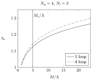
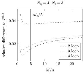
Figure 1: Perturbative decoupling of the charm quark. The factor $P_{3,4}$ (left plot) and the corrections $(P_{3,4}-P_{3,4}^{(1)})/P_{3,4}^{(1)}$ for different loop orders relative to the one-loop “approximation” $P_{3,4}^{(1)}=(M/\Lambda)^{2/27}$ (right plot).

For numerical applications we expand the integrands in Eq. (11) and Eq. (15) using Eq. (10) and Eq. (14) and we evaluate the integrals numerically. For the $n$-loop expression we set $b_{i}=0$, $d_{i-1}=0$ for $i\geq n$. A one-loop “approximation” is defined by setting $b_{i}=0\,,i>0$, $d_{i}=0$ :

$$P_{\mathrm{l},\mathrm{q}}^{(1)}=(M/\Lambda)^{\eta_{0}}\,,$$ (17)

where $\eta_{0}=1-{b_{0}(N_{\mathrm{q}})\over b_{0}(N_{\mathrm{l}})}>0$. In Fig. 1 we show the convergence of the perturbative expression for $P_{3,4}$, i.e., for the case of decoupling of the charm quark. The one-loop “approximation” is accidentally very close to the four-loop result. In the right plots of Fig. 1 we show the relative correction $(P_{3,4}-P_{3,4}^{(1)})/P_{3,4}^{(1)}$ where $P_{3,4}$ is computed to $n$-loops ($n=2,3,4$). The perturbative expansion appears to behave well even for the case of the charm quark, where one would not have necessarily expected it to be so. More details on the calculation of $P_{\mathrm{l},\mathrm{q}}$ will be presented in [10].

4 Non-perturbative results

In order to check the factorisation formula Eq. (3) and the applicability of perturbation theory to compute the factor $P_{\mathrm{l},\mathrm{q}}$ Eq. (12), we study a theory with $N_{\mathrm{q}}=2$ heavy quarks and compare it to Yang-Mills theory ($N_{\mathrm{l}}=0$). We simulate $N_{\mathrm{q}}=2$ O($a$) improved Wilson quarks [11] with plaquette gauge action. The ensembles are listed in Table 1. The simulations with periodic boundary conditions (p) are done with the MP-HMC algorithm [12] and those with open boundary conditions (o) with the publicly available openQCD package [13]. We refer to [3] for further explanations.

$\beta$	$a$ [${\rm fm}$]	BC	$T\times L^{3}$	$M/\Lambda_{\rm\overline{MS\kern-0.35002pt}\kern 0.35002pt}$	kMDU	$\tau_{\rm exp}$
$5.3$	$0.0658(10)$	p	$64\times 32^{3}$	0.638(46)	1.0	0.07
		p	$64\times 32^{3}$	1.308(95)	2.0	0.05
		p	$64\times 32^{3}$	2.60(19)	2.0	0.04
$5.5$	$0.0486($0$7)$	o	$120\times 32^{3}$	0.630(46)	8.5	0.15
		o	$120\times 32^{3}$	1.282(93)	8.1	0.12
		p	$96\times 48^{3}$	2.45(18)	4.0	0.10
$5.7$	$0.0341($0$5)$	o	$192\times 48^{3}$	0.587(43)	4.0	0.28
		o	$192\times 48^{3}$	1.277(94)	4.2	0.24
		o	$192\times 48^{3}$	2.50(18)	8.5	0.20

Table 1: The decoupling ensembles.

We consider the scale $m^{\mathrm{had}}=1/\sqrt{t_{0}}$ defined from the Wilson flow [5]. The factorisation formula for its mass-dependence reads, cf. Eq. (3)

$$\sqrt{t_{0}(M)/t_{0}(0)}=1/(P_{0,2}Q^{\sqrt{t_{0}}}_{0,2})+{\rm O}((\Lambda/M)^{2})$$ (18)

We compute from the simulations $t_{0}(M)/a^{2}$ at three values of the heavy quark mass close to the target values $M_{\mathrm{t}}/\Lambda=0.59$, $1.28$ and $2.50$. They correspond to approximately $M_{\rm c}/8$, $M_{\rm c}/4$ and $M_{\rm c}/2$ ($M_{\rm c}$ is the charm quark mass).

The RGI mass $M$ and the ratio $M/\Lambda$ are computed as explained in [3]. The data of the simulations in Table 1 are corrected for small mismatches compared to the target values $M_{\mathrm{t}}/\Lambda$. This is done by fitting the $\beta=5.7$ data to the form

$$t_{0}(M)/a^{2}=s_{1}\left(M/\Lambda\right)^{\alpha}\,.$$ (19)

We get $\alpha=-0.246(5)$ which is close to $-2\eta_{0}=-0.242424$. The corrected values $t_{0}(M_{\mathrm{t}})$ are computed as

$$\ln(t_{0}(M_{\mathrm{t}})/a^{2})=\ln(t_{0}(M)/a^{2})+\alpha\ln(M_{\mathrm{t}}/M)\,.$$ (20)

In order to keep the O($a$) improved coupling $\tilde{g}_{0}^{2}=(1+b_{g}(g_{0}^{2})N_{\mathrm{q}}am)g_{0}^{2}$ fixed, we correct

$$t_{0}(M_{\mathrm{t}})/a^{2}\longrightarrow(1+2\times 0.098N_{\mathrm{q}}am)\,t_{0}(M_{\mathrm{t}})/a^{2}\,,$$ (21)

where $m$ is the PCAC mass.

In order to compute the ratio in Eq. (18) we need the value $t_{0}(0)/a^{2}$ in the chiral limit. The latter is known only for $\beta=5.3$ and $\beta=5.5$ from [14]. For our smallest lattice spacing $a(\beta=5.7)$ we use

$$\left.\sqrt{t_{0}(M)/t_{0}(0)}\right|_{a(5.7)}\approx\left.\sqrt{t_{0}(M)/t_{0}(M_{\rm ref})}\right|_{a(5.7)}\times\lim_{a\to a(5.7)}\sqrt{t_{0}(M_{\rm ref})/t_{0}(0)}\,,$$ (22)

where the reference mass is chosen to be our lightest mass $M_{\rm ref}/\Lambda=0.59$. The limit in the second factor in Eq. (22) is computed by a linear extrapolation of the data $\sqrt{t_{0}(M_{\rm ref})/t_{0}(0)}$ at $\beta=5.3$ and $5.5$ as a function of $a^{2}/(8t_{0}(M_{\rm ref}))$. We add to the error of the extrapolation half of the difference between the $\beta=5.7$ and $\beta=5.5$ values. This error is added linearly to the total error in Eq. (22).

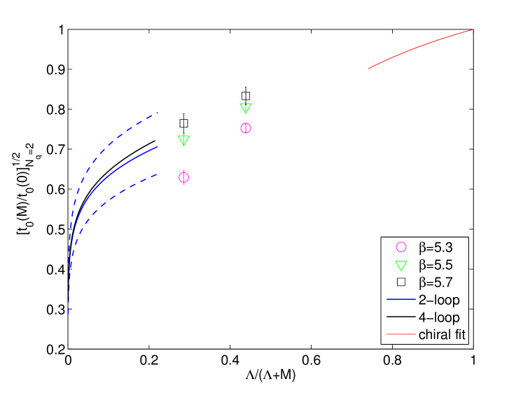
Figure 2: The mass dependence of the ratio $\sqrt{t_{0}(M)/t_{0}(0)}$.

The results for the ratio $\sqrt{t_{0}(M)/t_{0}(0)}$ at $M_{\mathrm{t}}/\Lambda=1.28$ and $2.50$ are shown by the symbols in Fig. 2. We compare them to the factorisation formula Eq. (18), where the factor $P_{0,2}$ is computed to 2- (blue line) and 4-loops (black line). The error on the factorization formula comes from $Q^{\sqrt{t_{0}}}_{0,2}=[\sqrt{t_{0}(0)}\Lambda]_{N_{\mathrm{q}}=2}/[\sqrt{t_{0}}\Lambda]_{N_{\mathrm{q}}=0}\simeq 1.19(13)$ and is displayed by the dashed blue lines only for the 2-loop curve. The value of $Q^{\sqrt{t_{0}}}_{0,2}$ is obtained from $Q^{r_{0}}_{0,2}=[\Lambda r_{0}(0)]_{N_{\mathrm{q}}=2}/[\Lambda r_{0}]_{N_{\mathrm{q}}=0}=1.30(14)$ known from previous works [15, 16] and $[\sqrt{t_{0}(0)}/r_{0}(0)]_{N_{\mathrm{q}}=2}/[\sqrt{t_{0}}/r_{0}]_{N_{\mathrm{q}}=0}\simeq 0.915$ from [17]. Within 10% accuracy, the perturbative prediction for the mass dependence of $\sqrt{t_{0}(M)/t_{0}(0)}$ agrees with our simulation results at $\beta=5.7$ for masses of about half the charm quark mass. For completeness, in Fig. 2 the red line to the right shows the mass dependence in the chiral limit [17, 14].

5 Conclusions

Perturbation theory seems to be reliable for decoupling of heavy quarks at leading order in $1/M$ even at the charm quark mass. Our data from simulations of $N_{\mathrm{q}}=2$ O($a$) improved Wilson quarks shown in Fig. 2 match the factorisation formula Eq. (3) for the mass dependence of hadronic scales. A careful continuum limit of the data in Fig. 2 will be addressed in the near future combined with twisted mass simulations.

Acknowledgements. We gratefully acknowledge the computer resources granted by the Gauss Centre for Supercomputing (GCS) through the John von Neumann Institute for Computing (NIC) on the GCS share of the supercomputer JUQUEEN at JSC, with funding by the German Federal Ministry of Education and Research (BMBF) and the German State Ministries for Research of Baden-Württemberg (MWK), Bayern (StMWFK) and Nordrhein-Westfalen (MIWF). We are further grateful for computer time allocated for our project on the Konrad and Gottfried computers at the North-German Supercomputing Alliance HLRN and on the Cheops computer at the University of Cologne (financed by the Deutsche Forschungsgemeinschaft). This work is supported by the Deutsche Forschungsgemeinschaft in the SFB/TR 09 and the SFB/TR 55.

References

• [1] S. Weinberg, Phenomenological Lagrangians, Physica A96 (1979) 327.
• [2] ALPHA Collaboration, M. Bruno, J. Finkenrath, F. Knechtli, B. Leder and R. Sommer, Effects of Heavy Sea Quarks at Low Energies, Phys. Rev. Lett. 114 (2015) 102001 arXiv:1410.8374 [hep-lat].
• [3] F. Knechtli, A. Athenodorou, M. Bruno, J. Finkenrath, F. Knechtli, B. Leder, M. Marinkovic and R. Sommer, Physical and cut-off effects of heavy sea quarks, PoS LATTICE2014 (2014) 288, [arXiv:1411.1239].
• [4] R. Sommer, A new way to set the energy scale in lattice gauge theories and its applications to the static force and $\alpha_{s}$ in SU(2) Yang-Mills theory, Nucl. Phys. B 411 (1994) 839 [hep-lat/9310022].
• [5] M. Lüscher, Properties and uses of the Wilson flow in lattice QCD, JHEP 1008 (2010) 071 [arXiv:1006.4518].
• [6] S. Weinberg, Effective gauge theories, Phys. Lett. B 91 (1980) 51.
• [7] W. Bernreuther and W. Wetzel, Decoupling of Heavy Quarks in the Minimal Subtraction Scheme, Nucl. Phys. B 197 (1982) 228.
• [8] A. G. Grozin, M. Hoeschele, J. Hoff, and M. Steinhauser, Simultaneous decoupling of bottom and charm quarks, JHEP 1109 (2011) 066 [arXiv:1107.5970].
• [9] K. Chetyrkin, J. H. Kühn, and C. Sturm, QCD decoupling at four loops, Nucl. Phys. B 744 (2006) 121, [hep-ph/0512060].
• [10] A. Athenodorou, M. Bruno, J. Finkenrath, F. Knechtli, B. Leder, M. Marinkovic and R. Sommer, The decoupling of heavy sea quarks, in preparation.
• [11] ALPHA Collaboration, K. Jansen and R. Sommer, O($a$) improvement of lattice QCD with two flavors of Wilson quarks, Nucl. Phys. B 530 (1998) 185, [hep-lat/9803017].
• [12] M. Marinkovic and S. Schaefer, Comparison of the mass preconditioned HMC and the DD-HMC algorithm for two-flavour QCD, PoS LATTICE2010 (2010) 031, [arXiv:1011.0911].
• [13] M. Lüscher and S. Schaefer, Lattice QCD with open boundary conditions and twisted-mass reweighting, Comput. Phys. Commun. 184 (2013) 519, [arXiv:1206.2809].
• [14] M. Bruno and R. Sommer, On the $N_{f}$-dependence of gluonic observables, PoS LATTICE2013 (2014) 321, [1311.5585].
• [15] ALPHA Collaboration, S. Capitani, M. Lüscher, R. Sommer, and H. Wittig, Non-perturbative quark mass renormalization in quenched lattice QCD, Nucl. Phys. B 544 (1999) 669, [hep-lat/9810063].
• [16] ALPHA Collaboration, P. Fritzsch, F. Knechtli, B. Leder, M. Marinkovic, S. Schaefer, R. Sommer and F. Virotta, The strange quark mass and Lambda parameter of two flavor QCD, Nucl. Phys. B 865 (2012) 397, [arXiv:1205.5380].
• [17] R. Sommer, Scale setting in lattice QCD, PoS LATTICE2013 (2014) 015, [arXiv:1401.3270].