Microscopic Theory of Traffic Flow Instability Governing Traffic Breakdown at Highway Bottlenecks: Growing Wave of Increase in Speed in Synchronized Flow

Abstract

We have revealed a growing local speed wave of increase in speed that can randomly occur in synchronized flow (S) at a highway bottleneck. The development of such a traffic flow instability leads to free flow (F) at the bottleneck; therefore, we call this instability as an S$\rightarrow$F instability. Whereas the S$\rightarrow$F instability leads to a local increase in speed (growing acceleration wave), in contrast, the classical traffic flow instability introduced in 50s–60s and incorporated later in a huge number of traffic flow models leads to a growing wave of a local decrease in speed (growing deceleration wave). We have found that the S$\rightarrow$F instability can occur only, if there is a finite time delay in driver over-acceleration. The initial speed disturbance of increase in speed (called $``$speed peak”) that initiates the S$\rightarrow$F instability occurs usually at the downstream front of synchronized flow at the bottleneck. There can be many speed peaks with random amplitudes that occur randomly over time. It has been found that the S$\rightarrow$F instability exhibits the nucleation nature: Only when a speed peak amplitude is large enough, the S$\rightarrow$F instability occurs; in contrast, speed peaks of smaller amplitudes cause dissolving speed waves of a local increase in speed (dissolving acceleration waves) in synchronized flow. We have found that the S$\rightarrow$F instability governs traffic breakdown – a phase transition from free flow to synchronized flow (F$\rightarrow$S transition) at the bottleneck: The nucleation nature of the S$\rightarrow$F instability explains the metastability of free flow with respect to an F$\rightarrow$S transition at the bottleneck.

I Introduction

In 1958–1961, Herman, Gazis, Montroll, Potts, Rothery, and Chandler GH195910 ; Gazis1961A10 ; GH10 ; Chandler from General Motors (GM) Company revealed the existence of a traffic flow instability associated with a driver over-deceleration effect: If a vehicle begins to decelerate unexpectedly, then due to a finite driver reaction time the following vehicle starts deceleration with a delay. As a result, the speed of the following vehicle becomes lower than the speed of the preceding vehicle. If this over-deceleration effect is realized for all following drivers, the traffic flow instability occurs leading to a growing wave of a local speed decrease in traffic flow that can be considered $``$growing deceleration wave” in traffic flow. With the use of very different mathematical approaches, this classical traffic flow instability has been incorporated in a huge number of traffic flow models; examples are well-known Kometani-Sasaki model KS ; KS1959A , optimal velocity (OV) model by Newell Newell1961 ; Newell1963A ; Newell1981 , a stochastic version of Newell’s model Newell_Stoch , Gipps model Gipps ; Gipps1986 , Wiedemann’s model Wiedemann , Whitham’s model Whitham1990 , Payne’s macroscopic model ach_Pay197110 ; ach_Pay197910 , the Nagel-Schreckenberg (NaSch) cellular automaton (CA) model Stoc , the OV model by Bando et al. Bando1995 , a stochastic model by Krauß et al. ach_Kra10 , a lattice model by Nagatani fail_Nagatani1998A ; fail_Nagatani1999B , Treiber’s intelligent driver model ach_Helbing200010 , the Aw-Rascle macroscopic model ach_Aw200010 , a full velocity difference OV model by Jiang et al. ach_Jiang2001A and a huge number of other traffic flow models (see references in books and reviews Reviews ; Reviews2 ; Kerner_Review ). All these different traffic flow models can be considered belonging to the same GM model class. Indeed, as found firstly in 1993–1994 KK1993 , in all these very different traffic flow models the classical instability leads to a moving jam (J) formation in free flow (F) (F$\rightarrow$J transition) (see references in Reviews2 ; KernerBook ; KernerBook2 ; Kerner_Review ). The classical instability of the GM model class should explain traffic breakdown, i.e., a transition from free flow to congested traffic observed in real traffic GH195910 ; Gazis1961A10 ; GH10 ; Chandler ; KS ; KS1959A ; Newell1961 ; Newell1963A ; Newell1981 ; Newell_Stoch ; Gipps ; Gipps1986 ; Wiedemann ; Whitham1990 ; ach_Pay197110 ; ach_Pay197910 ; Stoc ; Bando1995 ; ach_Kra10 ; fail_Nagatani1998A ; fail_Nagatani1999B ; ach_Helbing200010 ; ach_Aw200010 ; ach_Jiang2001A ; Reviews ; Reviews2 ).

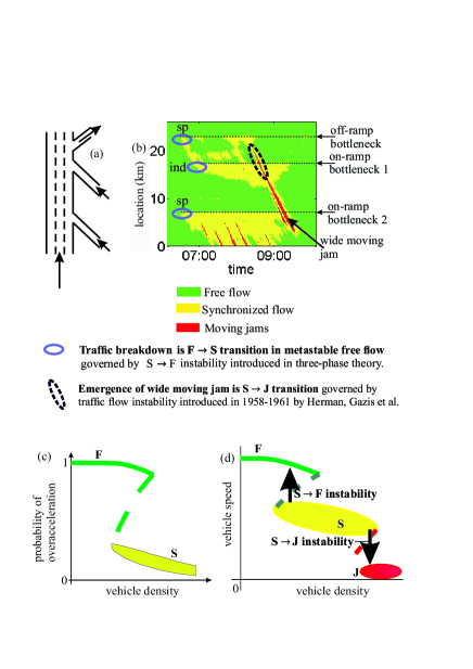
Figure 1: A known empirical example of phase transitions in traffic flow illustrating two traffic flow instabilities of three-phase theory (real measured traffic data of road detectors installed along three-lane highway) (a, b) Kerner_2014 and illustrations of associated hypotheses of three-phase theory (c, d): (a) Sketch of section of three-lane highway in Germany with three bottlenecks. (b) Speed data measured with road detectors installed along road section in (a); data KernerBook are presented in space and time with averaging method described in Sec. C.2 of KernerRSch2013 . (c) Hypothesis of three-phase theory about discontinuous character of over-acceleration probability Kerner1999A ; Kerner1999B ; Kerner1999C ; KernerBook ; KernerBook2 . (d) Hypothesis of three-phase theory about F$\rightarrow$S$\rightarrow$J phase transitions in traffic flow: 2Z-characteristic for phase transitions KernerBook ; Kerner1999B . F – free flow phase, S – synchronized flow phase, J – wide moving jam phase. In (b), $``$sp” – spontaneous F$\rightarrow$S transition, $``$ind” – induced F$\rightarrow$S transition KernerBook .

However, as shown in KernerBook ; KernerBook2 ; Kerner_Review , traffic flow models models of the GM model class (see references in Kerner_Review ; KernerBook ; KernerBook2 ) failed in the explanation of real traffic breakdown. This is because rather than an F$\rightarrow$J transition of the models of the GM model class, in all real field traffic data traffic breakdown is a phase transition from a metastable free flow to synchronized flow (F$\rightarrow$S transition) KR1997 ; Kerner1997A7 ; Kerner1998B ; Kerner1999A ; Kerner1999B ; Kerner1999C ; KernerBook ; KernerBook2 ; Kerner_Review ; Kerner2002A ; Waves ; Kerner_Review2 .

To explain an F$\rightarrow$S transition in metastable free flow, a three-phase traffic theory ($``$three-phase theory” for short) has been introduced Kerner1997A7 ; Kerner1998B ; Kerner1999A ; Kerner1999B ; Kerner1999C ; KernerBook ; KernerBook2 ; Kerner_Review which in addition to the free flow phase (F), there are two phases in congested traffic: the synchronized flow (S) and wide moving jam (J) phases. One of the characteristic features of the three-phase theory is the assumption about the existence of two qualitatively different instabilities in vehicular traffic:

(i) A traffic flow instability predicted in three-phase theory Kerner1999A ; Kerner1999B ; Kerner1999C ; KernerBook ; KernerBook2 ; Kerner_Review that is associated with an over-acceleration effect. It is assumed that probability of over-acceleration should exhibit a discontinuous character Kerner1999A ; Kerner1999B ; Kerner1999C ; KernerBook ; KernerBook2 (Fig. 1 (c)). Due to the discontinuous character of the over-acceleration probability the instability (labeled by S$\rightarrow$F instability in Fig. 1 (d)) should cause a growing wave of a local increase in the vehicle speed in synchronized flow. Respectively, in the three-phase theory it is assumed that a spatiotemporal competition between the over-acceleration effect and the speed adaptation effect occurring in car-following leads to the metastability of free flow with respect to an F$\rightarrow$S transition at the bottleneck. The assumption that traffic breakdown at a highway bottleneck is the F$\rightarrow$S transition occurring in metastable free flow is the basic assumption of the three-phase theory Kerner1999A ; Kerner1999B ; Kerner1999C ; KernerBook ; KernerBook2 ; Kerner_Review .

(ii) In the three-phase theory it is further assumed that rather than traffic breakdown, the instability of the GM model class explains a phase transition from synchronized flow to wide moving jams (S$\rightarrow$J transition) that is labeled by S$\rightarrow$J instability in Fig. 1 (d).

The first mathematical implementation of these hypotheses of three-phase theory Kerner1997A7 ; Kerner1998B ; Kerner1999A ; Kerner1999B ; Kerner1999C ; KernerBook ; KernerBook2 has been a stochastic continuous in space microscopic model KKl and a CA three-phase model KKW , which has been further developed for different applications in KKl2003A ; Kerner2008A ; Kerner2008B ; Kerner2008C ; Kerner2008D ; KKl2009A ; Kerner_2014 ; KKl2004A ; Kerner_Hyp ; KKHS2013 ; KKS2014A ; Heavy ; KKS2011 ; KKl2006AA ; Kerner_EPL ; Kerner_Diff . Over time there has been developed a number of other three-phase flow models (e.g., Davis ; Lee_Sch2004A ; Jiang2004A ; Gao2007 ; Davis2006 ; Davis2006b ; Davis2006d ; Davis2006e ; Davis2010 ; Davis2011 ; Jiang2007A ; Jiang2005A ; Jiang2005B ; Jiang2007C ; Pott2007A ; Li ; Wu2008 ; Laval2007A8 ; Hoogendoorn20088 ; Wu2009 ; Jia2009 ; Tian2009 ; He2009 ; Jin2010 ; Klenov ; Klenov2 ; Kokubo ; LeeKim2011 ; Jin2011 ; Neto2011 ; Zhang2011 ; Wei-Hsun2011IEEEA ; Lee2011A ; Tian2012 ; Kimathi2012B ; Wang2012A ; Tian2012B ; Qiu2013 ; YangLu2013A ; KnorrSch2013A ; XiangZhengTao2013A ; Mendez2013A ; Rui2014A ; Hausken2015A ; Tian2015A ; Rui2015A ; Rui2015B ; Rui2015C ; Rui2015D ; Xu2015A ; Davis2015A ) that incorporate some of the hypotheses of the three-phase theory Kerner1999A ; Kerner1999B ; Kerner1999C ; KernerBook ; KernerBook2 .

The hypothesis that the S$\rightarrow$F instability at a highway bottleneck should govern the nucleation nature of an F$\rightarrow$S transition, i.e., the metastability of free flow with respect to an F$\rightarrow$S transition (traffic breakdown) was introduced in the three-phase theory many years ago Kerner1999A ; Kerner1999B ; Kerner1999C ; KernerBook (Fig. 1 (d)). However, microscopic physical features of this S$\rightarrow$F instability have been unknown up to now. In particular, the following theoretical questions arise, which have not been answered in earlier theoretical studies of three-phase flow models KernerBook ; KernerBook2 ; KKl ; KKl2003A ; Kerner2008A ; Kerner2008B ; Kerner2008C ; Kerner2008D ; KKl2009A ; Kerner_2014 ; KKl2004A ; KKHS2013 ; KKS2014A ; Heavy ; KKS2011 ; KKW ; KKl2006AA ; Kerner_Diff :

(i) What is a disturbance in synchronized flow that can spontaneously initiate the S$\rightarrow$F instability at the bottleneck?

(ii) Can be proven that the S$\rightarrow$F instability at the bottleneck exhibits the nucleation nature?

(iii) How does the S$\rightarrow$F instability occurring in synchronized flow governs the metastability of free flow with respect to the F$\rightarrow$S transition at the bottleneck? Indeed, in accordance with in the three-phase theory KernerBook the speed adaptation effect, which describes the tendency from free flow to synchronized flow, cannot lead to some traffic flow instability. Therefore, the speed adaptation effect cannot be the origin of the nucleation nature of the F$\rightarrow$S transition at the bottleneck observed in real traffic.

(iv) What is the physics of a random time delay to the F$\rightarrow$S transition at the bottleneck found in simulations with stochastic three-phase traffic flow models KernerBook ; KernerBook2 ; KKl2003A ; Kerner2008A ; Kerner2008B ; Kerner2008C ; Kerner2008D ; KKl2009A ; Kerner_2014 ; KKl2004A ; KKHS2013 ; KKS2014A ; Heavy ; KKS2011 ; KKW ?

In this article, we reveal microscopic features of the S$\rightarrow$F instability that answer the above questions (i)–(iv). We will show that this microscopic theory of the S$\rightarrow$F instability exhibits a general character: All results can be derived with very different mathematical stochastic three-phase traffic flow models, in particular with the KKSW (Kerner-Klenov-Schreckenberg-Wolf) CA model KKW ; KKHS2013 ; KKS2014A and the Kerner-Klenov stochastic model KKl ; KKl2003A ; KKl2009A ; Kerner_2014 ; KKl2004A ; Heavy . Because the KKSW CA model is considerably more simple one than the Kerner-Klenov stochastic model, we present results of the microscopic theory of the S$\rightarrow$F instability based on a study on the KKSW CA model; associated results derived with the Kerner-Klenov stochastic model are briefly considered in discussion section.

The article is organized as follows. In Sec. II, we show the existence of an S$\rightarrow$F instability at a highway bottleneck. The nucleation nature of an S$\rightarrow$F instability at the bottleneck is the subject of Sec. III. Microscopic features of a random time-delayed traffic breakdown (F$\rightarrow$S transition) at highway bottlenecks are studied in Sec. IV. This analysis proves that the S$\rightarrow$F instability governs traffic breakdown at the bottleneck. A general character of this conclusion is shown in Sec. V. In Sec. VI, we compare the classical traffic flow instability of the GM model class with the S$\rightarrow$F instability of three-phase theory (Sec. VI.1), discuss cases in which either there is no over-acceleration in the KKSW CA model (Sec. VI.2) or there is no time delay in over-acceleration in the KKSW CA model (Sec. VI.3), make a generalization of the results based on an analysis of the Kerner-Klenov stochastic model (Sec. VI.4) as well as formulate conclusions (Sec. VI.5).

II S$\rightarrow$F Traffic Flow Instability

II.1 KKSW CA Model

To study the S$\rightarrow$F traffic flow instability in synchronized flow at a highway bottleneck, we use the KKSW CA three-phase traffic flow model KKW ; KKHS2013 ; KKS2014A whose parameters are the same as those in KKS2014A .

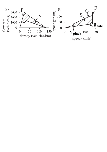
Figure 2: Steady states of the KKSW CA model in the flow–density (a) and space-gap–speed planes (b). $G$ and $g_{\rm safe}$ are, respectively, a synchronization gap and a safe gap at a time-independent speed $v$ (where $g_{\rm safe}=v$), F – free flow, S – synchronized flow (hatched 2D-regions in (a, b)). Parameters of the KKSW CA model used in simulations are as follows: $d=$ 5 (7.5 m), $v_{\rm free}=$ 25 (135 km/h), $p_{3}=$ 0.01, $p^{(2)}_{0}=$ 0.5, $v_{\rm pinch}=$ 8 (43.2 km/h), $k_{1}=$ 3, $k_{2}=$ 2. $p_{\rm a,1}=$0.07, $p_{\rm a,2}=$0.08, $p^{(2)}_{2}=$0.35, $v_{\rm syn}=$14 (75.6 km/h), $\Delta v_{\rm syn}=$3 (16.2 km/h).

II.1.1 Rules of vehicle motion in KKSW CA model

In the KKSW CA model for identical drivers and vehicles moving on a single-lane road KKS2014A , the following designations for main variables and vehicle parameters are used: $n=0,1,2,...$ is the number of time steps; $\tau=1$ s is time step; $\delta x=1.5$ m is space step; $x_{n}$ and $v_{n}$ are the coordinate and speed of the vehicle; time and space are measured in units of $\tau$ and $\delta x$, respectively; $v_{\rm free}$ is the maximum speed in free flow; $g_{n}=x_{\ell,n}-x_{n}-d$ is a space gap between two vehicles following each other; the lower index $\ell$ marks variables related to the preceding vehicle; $d$ is vehicle length; $G_{n}$ is a synchronization space gap (Fig. 2 (a, b)).

The KKSW CA model consists of the following sequence of rules KKS2014A :

(a) $``$comparison of vehicle gap with the synchronization gap”:

$$\quad\mbox{if}\ g_{n}\leq G(v_{n})$$

then follow rules (b), (c) and skip rule (d), (1)

$$\quad\mbox{if}\ g_{n}>G(v_{n})$$

then skip rules (b), (c) and follow rule (d), (2)

(b) $``$speed adaptation within synchronization gap” is given by formula:

$$v_{n+1}=v_{n}+\mathrm{sgn}(v_{\ell,n}-v_{n}),$$ (3)

(c) $``$over-acceleration through random acceleration within synchronization gap” is given by formula

$$\mbox{if}\ v_{n}\geq v_{\ell,n},\ \mbox{then with probability}\ p_{\rm a},$$

$$\quad v_{n+1}=\min(v_{n+1}+1,\ v_{\rm free}),$$ (4)

(d) $``$acceleration”:

$$v_{n+1}=\min(v_{n}+1,\ v_{\rm free}),$$ (5)

(e) $``$deceleration”:

$$v_{n+1}=\min(v_{n+1},\ g_{n}),$$ (6)

(f) $``$randomization” is given by formula:

$${\rm with}\ {\rm probability}\ p,\quad v_{n+1}=\max(v_{n+1}-1,\ 0),$$ (7)

(g) $``$motion” is described by formula:

$$x_{n+1}=x_{n}+v_{n+1}.$$ (8)

Formula (II.1.1) is applied, when

$$r<p_{\rm a},$$ (9)

formula (7) is applied, when

$$p_{\rm a}\leq r<p_{\rm a}+p,$$ (10)

where $p_{\rm a}+p\leq 1$; $r=rand()$ is a random value distributed uniformly between 0 and 1. Probability of over-acceleration $p_{\rm a}$ in (II.1.1) is chosen as the increasing speed function:

$$p_{\rm a}(v_{n})=p_{\rm a,1}+p_{\rm a,2}\max(0,\min(1,\ (v_{n}-v_{\rm syn})/\Delta v_{\rm syn})),$$ (11)

where $p_{\rm a,1}$, $p_{\rm a,2}$, $v_{\rm syn}$ and $\Delta v_{\rm syn}$ are constants. In (II.1.1), (II.1.1),

$$G(v_{n})=kv_{n}.$$ (12)

The rules of vehicle motion (II.1.1)–(12) (without formula (11)) have been formulated in the KKW (Kerner-Klenov-Wolf) CA model KKW . In comparison with the KKW CA model KKW , we use in (7), (10) for probability $p$ formula

$$p=\left\{\begin{array}[]{ll}p_{2}&\textrm{for $v_{n+1}>v_{n}$},\\ p_{3}&\textrm{for $v_{n+1}\leq v_{n}$},\end{array}\right.$$ (13)

which has been used in the KKSW CA model of Ref. KKHS2013 . The importance of formula (13) is as follows. This rule of vehicle motion leads to a time delay in vehicle acceleration at the downstream front of synchronized flow. In other words, this is an additional mechanism of time delay in vehicle acceleration in comparison with a well-known slow-to-start rule Stoc2 ; Schadschneider_Book :

$$p_{2}(v_{n})=\left\{\begin{array}[]{ll}p^{(2)}_{0}&\textrm{for $v_{n}=0$},\\ p^{(2)}_{1}&\textrm{for $v_{n}>0$}\\ \end{array}\right.$$ (14)

that is also used in the KKSW CA model. However, in the KKSW CA model in formula (14) probability $p^{(2)}_{1}$ is chosen to provide a delay in vehicle acceleration only if the vehicle does not accelerate at previous time step $n$:

$$p^{(2)}_{1}=\left\{\begin{array}[]{ll}p^{(2)}_{2}&\textrm{for $v_{n}\leq v_{n-1}$},\\ 0&\textrm{for $v_{n}>v_{n-1}$}.\\ \end{array}\right.$$ (15)

In (13)–(15), $p_{3}$, $p^{(2)}_{0}$, and $p^{(2)}_{2}$ are constants. We also assume that in (12) KKW

$$k(v_{n})=\left\{\begin{array}[]{ll}k_{1}&\textrm{for $v_{n}>v_{\rm pinch}$},\\ k_{2}&\textrm{for $v_{n}\leq v_{\rm pinch}$},\\ \end{array}\right.$$ (16)

where $v_{\rm pinch}$, $k_{1}$, and $k_{2}$ are constants ($k_{1}>k_{2}\geq 1$).

The rule of vehicle motion (13) of the KKSW CA model KKHS2013 together with formula (11) allows us to improve characteristics of synchronized flow patterns (SP) simulated with the KKSW CA model (II.1.1)–(16) for a single-lane road. Other physical features of the KKSW CA model have been explained in KKHS2013 . A model of an on-ramp bottleneck is the same as that presented in KKS2011 .

In accordance with qualitative three-phase theory KernerBook , a competition between speed adaptation and over-acceleration should determine the existence of an S$\rightarrow$F instability. Thus it is useful to discuss the description of these effects with the KKSW CA model.

II.1.2 Speed adaptation effect in KKSW CA model

In the KKSW CA model, the speed adaptation effect in synchronized flow takes place within the space gap range:

$$g_{\rm safe,\ n}\leq g_{\rm n}\leq G_{\rm n},$$ (17)

where $g_{\rm safe,\ n}$ is a safe space gap, $g_{\rm safe,\ n}=v_{n}$. Under condition (17), formula (3) is valid, i.e., the vehicle tends to adjust its speed to the preceding vehicle without caring, what the precise space gap is, as long as it is safe: The vehicle accelerates or decelerates in dependence of whether the vehicle moves slower or faster than the preceding vehicle, respectively. In other words, there are both $``$negative” and $``$positive” speed adaptation.

II.1.3 Time delay in over-acceleration in KKSW CA model

A formulation for model fluctuations that simulates over-acceleration on a single-lane road is as follows. Each vehicle, which moves in synchronized flow with a space gap that satisfies conditions (17) (Fig. 2 (b)), accelerates randomly with some probability $p_{\rm a}$ (II.1.1). This random vehicle acceleration occurs only under conditions (17) and

$$v_{n}\geq v_{\ell,n}.$$ (18)

Thus the vehicle accelerates with probability $p_{\rm a}$, even if the preceding vehicle does not accelerate and the vehicle speed is not lower than the speed of the preceding vehicle. Therefore, in accordance with the definition of over-acceleration KernerBook ; KernerBook2 , this vehicle acceleration is an example of over-acceleration. Because the probability of over-acceleration $p_{\rm a}<1$, there is on average a time delay in over-acceleration. The mean time delay in the over-acceleration is longer than time step of the KKSW CA model ($\tau=$ 1 s). The over-acceleration effect results in the discontinuous character of the probability of over-acceleration as a density (and flow rate) function as required by the associated hypothesis of three-phase theory Kerner1999A ; Kerner1999B ; Kerner1999C ; KernerBook ; KernerBook2 (Fig. 1 (c)).

The probability of over-acceleration $p_{\rm a}$ (II.1.1) is an increasing function of vehicle speed. This model feature supports the over-acceleration within a local speed disturbance of increase in speed in synchronized flow. As predicted in KernerBook ; KernerBook2 , the stronger the over-acceleration, the more probable should be the occurrence of the S$\rightarrow$F instability.

II.2 Speed peak at downstream front of synchronized flow at on-ramp bottleneck

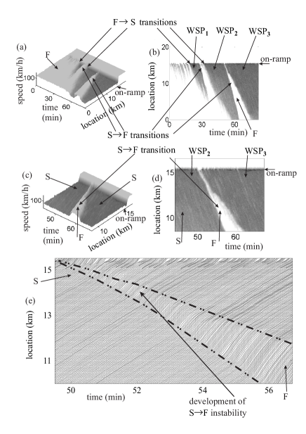
Figure 3: Simulations of the S$\rightarrow$F instability in synchronized flow leading to S$\rightarrow$F transition at on-ramp bottleneck on single-lane road with the KKSW CA model: (a–d) Speed in space and time (a, c) and the same speed data presented by regions with variable shades of gray (in white regions the speed is equal to or higher than 110 km/h, in black regions the speed is zero) (b, d); figures (c, d) are, respectively, fragments of (a, b) in larger scales in space and time. (e) Fragment of vehicle trajectories in space and time related to (c, d); bold dashed-dotted curves in (e) mark the development of S$\rightarrow$F instability in synchronized flow leading to S$\rightarrow$F transition. F – free flow, S – synchronized flow, WSP – widening synchronized flow pattern. $q_{\rm on}=$ 360 vehicles/h, $q_{\rm in}=$ 1406 vehicles/h. On-ramp location $x_{\rm on}=$ 15 km. Merging region of the on-ramp is located within 15 km $\leq x\leq$ 15.3 km (i.e., road locations within which vehicles can merge from the on-ramp lane onto the main road). Other model parameters are the same as those in Fig. 2.

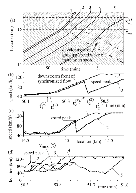
Figure 4: Speed peak at the downstream front of synchronized flow at bottleneck that initiates S$\rightarrow$F instability shown in Fig. 3 (c–e): (a) Fragment of vehicle trajectories related to Fig. 3 (e); bold dashed-dotted curves in (a) mark the development of the speed wave of increase in speed within synchronized flow. (b–d) Microscopic vehicle speed along trajectories as time-functions (b, d) and road location functions (c). In (b–d), vehicle trajectories are labeled by the same numbers as those in (a). $x_{\rm on}=$ 15 km and $x^{\rm(e)}_{\rm on}=15.3$ km are, respectively, the beginning and the end of the merging region of the on-ramp which which vehicles can merge from the on-ramp onto the main road.

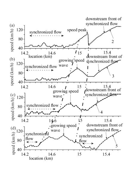
Figure 5: Transformation of speed peak shown in Fig. 4 (c) into a growing speed wave of increase in speed propagating upstream within synchronized flow: (a–d) Microscopic vehicle speeds along trajectories as road location-functions labeled by the same numbers as those in Fig. 4 (a). In (a–d), bold dashed-dotted curves mark a growing speed wave of increase in speed within synchronized flow as a function of road location.

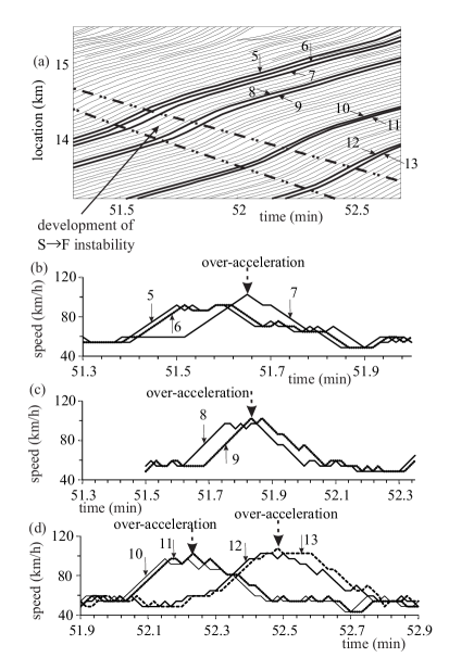
Figure 6: Effect of over-acceleration on S$\rightarrow$F instability shown in Fig. 3 (c–e): (a) Fragment of vehicle trajectories in space and time; bold dashed-dotted curves mark upstream propagation of the growing wave of increase in speed within synchronized flow. (b–d) Microscopic vehicle speed along trajectories as time functions labeled by the same numbers as those in (a).

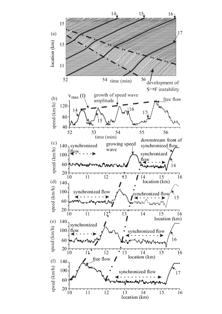
Figure 7: Subsequent development of S$\rightarrow$F instability, i.e., of growing speed wave of increase in speed within synchronized flow shown in Fig. 6 (a): (a) Fragment of vehicle trajectories in space and time; bold dashed-dotted curves in (a) mark the development of speed wave of increase in speed within synchronized flow. (b) Microscopic vehicle speeds along trajectories as time functions labeled by the same numbers as those in (a); bold dashed curve marks the increase of the wave amplitude over time $v_{\rm max}(t)$. (c–f) Microscopic vehicle speeds along trajectories as road location-functions labeled by the same numbers as those in (a); bold dashed-dotted curves mark the development of growing speed wave of increase in speed within synchronized flow as a function of road location.

In simulations of traffic flow on a single-lane road with an on-ramp bottleneck with the KKSW CA model, we find a sequence of F$\rightarrow$S and S$\rightarrow$F transitions at the bottleneck (labeled respectively by $``$F$\rightarrow$S transitions” and $``$S$\rightarrow$F transitions” in Fig. 3 (a–d)). At chosen flow rates $q_{\rm on}$ and $q_{\rm in}$ (Fig. 3), each of the F$\rightarrow$S transitions leads to the formation of a widening synchronized flow pattern (WSP) at the bottleneck (labeled by $``$$\rm WSP_{1}$”, $``$$\rm WSP_{2}$”, and $``$$\rm WSP_{3}$” in Fig. 3). To understand microscopic features of the S$\rightarrow$F instability, we consider of an S$\rightarrow$F transition shown in Fig. 3 (c, d).

Microscopic features of the S$\rightarrow$F instability (Fig. 3 (e)) are as follows. Firstly, a disturbance of increase in speed emerges at the downstream front of synchronized flow at the on-ramp bottleneck (Fig. 4). We call this disturbance as $``$speed peak” (labeled by $``$speed peak” on trajectory 2 in Figs. 4 (b–d)): At time instant $t=t^{(1)}_{1}$ vehicle 1 begins to accelerate at the downstream front of synchronized flow (Fig. 4 (b, c)). Within the downstream front of synchronized flow, vehicle 1 accelerates continuously from a synchronized flow speed to free flow downstream of the bottleneck. Vehicle 1 reaches a free flow speed at time instant $t^{(1)}_{2}$ (trajectory 1 in Fig. 4 (b)). A different situation is realized for vehicle 2 that follows vehicle 1 on the main road.

After vehicle 1 has begun to accelerate, vehicle 2 begins also to accelerate at the downstream front of synchronized flow at time instant $t^{(2)}_{1}$ (trajectory 2 in Fig. 4 (b)). However, a slower moving vehicle merges from on-ramp lane onto the main road between vehicles 1 and 2 (bold dotted vehicle trajectory between vehicle trajectories 1 and 2 in Fig. 4 (a)).

Because vehicles 1 and 2 move on single-lane road, vehicle 2 cannot overtake the vehicle merging from the on-ramp. As a result, vehicle 2 must decelerate at time $t^{(2)}_{2}$ (trajectory 2 in Fig. 4 (b)). After the vehicle merging from the on-ramp increases its speed considerably, vehicle 2 can continue acceleration to the free flow speed at time instant $t^{(2)}_{3}$ (trajectory 2 in Fig. 4 (b)). This effect leads to the occurrence of a speed peak at the downstream front of synchronized flow at the bottleneck (Fig. 4 (b)).

II.3 Over-acceleration effect as the reason of growing speed wave of increase in speed within synchronized flow

The speed peak initiates a speed wave of increase in speed within synchronized flow. This speed wave propagates upstream. This effect can be seen in Figs. 4(a, d) and 5. Firstly, while the wave propagates upstream, the maximum speed $v_{\rm max}$ within the wave does not change considerably (Fig. 4(d)).

Later, the speed wave begins to grow both in the amplitude and in the space (Figs. 5–7). Finally, the growth of the wave leads to an S$\rightarrow$F transition at the bottleneck. The S$\rightarrow$F instability, i.e., the growth of the speed wave of a local increase in speed within synchronized flow is caused by the over-acceleration effect. The growing speed wave of increase in speed in synchronized flow can also be considered $``$growing acceleration wave” in synchronized flow. To show the effect of over-acceleration on the S$\rightarrow$F instability, we consider vehicle trajectories 5–13 within the growing speed wave of increase in speed (Fig. 6).

The over-acceleration effect can be seen, if we compare the motion of vehicles 5, 6 with vehicle 7 that follow each other (Fig. 6 (a)) within the speed wave of increase in speed (Fig. 6 (b)). Whereas vehicle 6 follows vehicle 5 without over-acceleration, vehicle 7 accelerates while reaching the speed that exceeds the speed of preceding vehicle 6 appreciably (trajectories 6 and 7 in Fig. 6 (b)). Although vehicle 6 begins to decelerate, nevertheless vehicle 7 accelerates. This acceleration of vehicle 7 occurs under conditions (17) and (18). For this reason, the acceleration of vehicle 7 is an example of the over-acceleration effect (labeled by $``$over-acceleration” in Fig. 6 (b)).

The effect of over-acceleration exhibits also vehicle 9 that follows vehicle 8, vehicle 10 that follows vehicle 11 as well as vehicle 13 that follows vehicle 12 (trajectories 9–13 in Fig. 6 (c ,d)). The subsequent effects of over-acceleration of different vehicles leads to the S$\rightarrow$F instability, i.e., to a growing wave of the increase in speed within synchronized flow. The speed wave grows both in the amplitude and in the space extension during its upstream propagation within synchronized flow. The subsequent development of this traffic flow instability caused by the over-acceleration effect can be seen in Fig. 7.

III Nucleation Nature of S$\rightarrow$F Instability at Bottlenecks

III.1 Random sequence of speed peaks at downstream front of synchronized flow

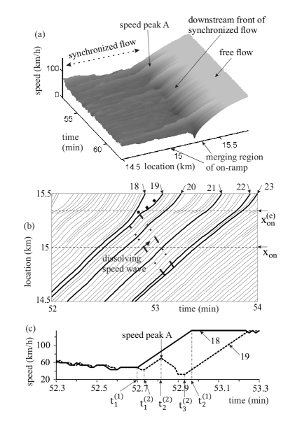
Figure 8: Speed peaks at downstream front of synchronized flow at the on-ramp bottleneck: (a) Speed in space and time; fragment of Fig. 3 (a) for a time interval that begins after time instant at which the S$\rightarrow$F instability at bottleneck has occurred; one of the speed peaks in (a) is marked by $``$speed peak A”. (b) Fragment of vehicle trajectories with a dissolving speed wave initiated by speed peak A in (a) (the dissolving wave is marked by dotted-dashed curves). (c) Microscopic vehicle speed along trajectories as time-functions showing the emergence of speed peak A; vehicle trajectories are labeled by the same numbers as those in (b). $x_{\rm on}=$ 15 km and $x^{\rm(e)}_{\rm on}=15.3$ km are, respectively, the beginning and the end of the merging region of the on-ramp within which vehicles can merge from the on-ramp onto the main road.

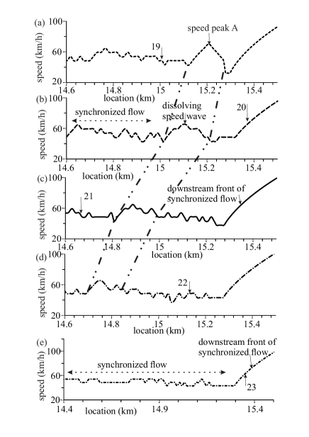
Figure 9: Dissolving speed wave within synchronized flow at the on-ramp bottleneck related to Fig. 8 (b, c): (a–e) Microscopic speed along vehicle trajectories as road location functions. Vehicle trajectories are labeled by the same numbers as those in Fig. 8 (b). Bold dashed-dotted curves mark the propagation of dissolving speed wave in space.

There can be many speed peaks that occur randomly at the downstream front of synchronized flow at the on-ramp bottleneck (Fig. 8 (a)). The physics of all speed peaks shown in Fig. 8 is the same as discussed above (Sec. II.2).

As an example, we consider a speed peak labeled by $``$speed peak A” in Fig. 8 (a). Due to slow vehicle merging from the on-ramp onto the main road (bold dotted vehicle trajectory between vehicle trajectories 18 and 19 in Fig. 8 (b)), vehicle 19 moving on the main road at time instant $t^{(2)}_{2}$ should change acceleration at the downstream front of synchronized flow to deceleration (Fig. 8 (c)); other time instants marked in Fig. 8 (c) have also the same sense as those in Fig. 4 (b). As a result of this deceleration of vehicle 19, speed peak A emerges (Fig. 8 (a, c)).

III.2 Dissolving speed wave of increase in speed within synchronized flow at bottleneck

Speed peak A initiates a speed wave of increase in speed within synchronized flow that propagates upstream. However, rather than an S$\rightarrow$F instability occurs discussed in Secs. II.2 and II.3, the wave is fully dissolved about 0.3 km upstream of the beginning of the on-ramp merging region at $x=$ 15 km. We call this wave as $``$dissolving speed wave” of increase in speed in synchronized flow (Figs. 8 (b) and 9 (e)).

The speed peak shown in Fig. 4, which initiates the S$\rightarrow$F instability (Secs. II.2 and II.3), and speed peak that does not initiate an S$\rightarrow$F instability differ in their amplitudes: The speed within the peak shown in Fig. 4 is about 98 km/h; the speed within peak A is considerably smaller (about 70 km/h). All other speed peaks that emerge at the downstream front of synchronized flow (Fig. 8 (a)) exhibit also considerably smaller amplitudes than that of the speed peak shown in Fig. 4. As a result, all waves of increase in speed within synchronized flow that the other speed peaks initiate are dissolving speed waves. A dissolving speed wave of increase in speed in synchronized flow can also be considered $``$dissolving acceleration wave” in synchronized flow.

We have found that if the speed peak amplitude is equal to or larger than some critical one, the speed peak is a nucleus for an S$\rightarrow$F instability (Secs. II.2 and II.3). Contrarily, if the peak amplitude is smaller than the critical one (as this is the case for all speed peaks in Fig. 8 (a)), the speed peak is smaller than a nucleus for an S$\rightarrow$F instability: Instead of the S$\rightarrow$F instability, the peak initiates a dissolving wave of the increase in speed within synchronized flow (Figs. 8 (b) and 9).

The physics of the nucleation nature of an S$\rightarrow$F instability is as follows. The over-acceleration effect is able to overcome speed adaptation between following each other vehicles (speed adaptation effect) only if the speed within the speed wave is large enough: When the over-acceleration effect is stronger than the speed adaptation effect within the speed wave, as that occurs in Fig. 6, the S$\rightarrow$F instability is realized. Otherwise, when during the speed wave propagation the speed adaptation effect suppresses the over-acceleration within synchronized flow, the speed wave dissolves over time, i.e., no S$\rightarrow$F instability is realized (Fig. 9(b–e)).

IV Random time-delayed traffic breakdown as result of S$\rightarrow$F instability

As already found in KKl ; KKW ; KKl2003A , there is a random time delay $T^{\rm(B)}$ between the beginning of a simulation realization and the time instant at which traffic breakdown (F$\rightarrow$S transition) occurs resulting in the emergence of a congested pattern at the bottleneck. At chosen flow rates $q_{\rm on}$ and $q_{\rm in}$, the congested pattern is an WSP (Fig. 10).

The microscopic nature of a random time delay of traffic breakdown at the bottleneck revealed below allows us to understand that and how an S$\rightarrow$F instability governs traffic breakdown. However, before we should understand microscopic features of traffic breakdown at the bottleneck (Sec. IV.1).

IV.1 Microscopic features of traffic breakdown (F$\rightarrow$S transition) at bottleneck

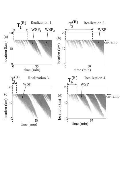
Figure 10: Random time delay of traffic breakdown (F$\rightarrow$S transition) at on-ramp bottleneck: (a–d) Speed in space and time for four different simulation realizations (runs) presented by regions with variable shades of gray (in white regions the speed is equal to or higher than 110 km/h, in black regions the speed is zero). Different realizations are made at the same model parameters, however, at different initial values $r$ in formulae (9) and (10) at time instant $t=0$. Realization 1 in (a) is a fragment of Fig. 3 (b), i.e., realization 1 is the simulation realization studied in Figs. 3–9. Time delays of traffic breakdown $T^{\rm(B)}$ in different simulation realizations 1–4 are $T^{\rm(B)}_{1}=$ 19 min (a), $T^{\rm(B)}_{2}=$35 min (b), $T^{\rm(B)}_{3}=$7 min (c), and $T^{\rm(B)}_{4}=$13 min (d). $q_{\rm on}=$ 360 vehicles/h, $q_{\rm in}=$ 1406 vehicles/h.

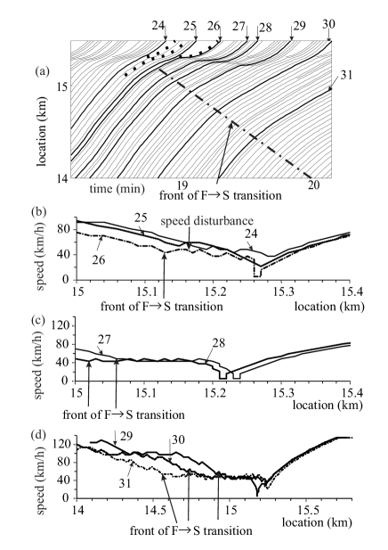
Figure 11: Traffic breakdown (F$\rightarrow$S transition) at on-ramp bottleneck that leads to the formation of ${\rm WSP_{1}}$ in Fig. 10 (a): (a) Fragments of vehicle trajectories related to Fig. 10 (a); bold dashed-dotted curve marks the propagation of the upstream front of synchronized flow (labeled by $``$front of F$\rightarrow$S transition”) in space and time. (b–d) Microscopic speed along vehicle trajectories as road location functions. Vehicle trajectories are labeled by the same numbers as those in (a).

We have found that in each of the simulation realizations (Fig. 10), traffic breakdown (F$\rightarrow$S transition) exhibits the following common microscopic features:

(i) Vehicles that merge onto the main road from the on-ramp (vehicle trajectories labeled by bold dotted curves in Fig. 11 (a)) force vehicles moving on the main road to decelerate strongly. This results in the formation of a speed disturbance of decrease in speed. The upstream front of the disturbance begins to propagate upstream of the bottleneck (labeled by $``$speed disturbance” on vehicle trajectory 26 in Fig. 11 (b)).

(ii) Due to speed adaptation of vehicles following this decelerating vehicle on the main road (vehicle trajectories 27–31 in Fig. 11 (a, c, d)), synchronized flow region appears that upstream front propagates upstream (labeled by $``$front of F$\rightarrow$S transition” in Fig. 11).

(iii) After traffic breakdown has occurred, many speed peaks appear in the synchronized flow at the bottleneck (not shown). The microscopic features of these peaks are qualitatively the same as those shown in Fig. 8 (a, c). In particular, the speed peaks lead to formation of a speed wave of increase in speed that propagates upstream within the synchronized flow. During a long enough time interval (time interval of the existence of $\rm WSP_{1}$ shown in Fig. 10 (a)), all speed waves are dissolving ones. The dissolving speed waves (not shown) exhibit the same microscopic features as those shown in Figs. 8 (b) and 9.

IV.2 Microscopic features of sequence of F$\rightarrow$S$\rightarrow$F transitions at bottleneck

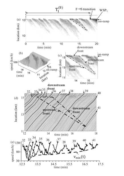
Figure 12: Simulations of F$\rightarrow$S$\rightarrow$F transitions within a permanent speed disturbance at on-ramp bottleneck: (a) Speed in space and time presented by regions with variable shades of gray (in white regions the speed is equal to or higher than 100 km/h, in black regions the speed is equal to 20 km/h) within time delay of traffic breakdown related to Fig. 10 (a). (b, c) Speed in space and time (b) and the same speed data presented by regions with variable shades of gray (c) for a short time interval in (a). (d) Fragment of vehicle trajectories in space and time related to (b, c). (e) Microscopic vehicle speeds along trajectories as time functions labeled by the same numbers as those in (d).

Figure 13: Simulations of an F$\rightarrow$S transition within a permanent speed disturbance (labeled by $``$permanent disturbance”) at on-ramp bottleneck: (a) Fragment of vehicle trajectories in space and time related to Fig. 12 (b, c). (b–f) Microscopic vehicle speeds along trajectories as road location-functions labeled by the same numbers as those in (a).

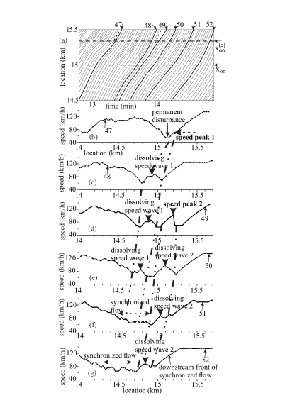
Figure 14: Simulations of speed peaks 1 and 2 with resulting dissolving speed waves 1 and 2 of increase in speed within synchronized flow at on-ramp bottleneck: (a) Fragment of vehicle trajectories in space and time related to Fig. 12 (b, c). (b–g) Microscopic vehicle speeds along trajectories as road location-functions labeled by the same numbers as those in (a).

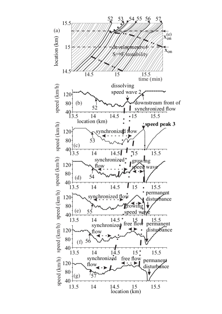
Figure 15: Simulations of a growing speed wave of increase in speed within synchronized flow at on-ramp bottleneck (region bounded by bold dashed-dotted curves labeled by $``$growing speed wave”): (a) Fragment of vehicle trajectories in space and time related to Fig. 12 (b, c). (b–g) Microscopic vehicle speeds along trajectories as road location-functions labeled by the same numbers as those in (a). A dissolving speed wave (region bounded by bold dashed-dotted curves labeled by $``$dissolving speed wave 2”) is a continuation of the dissolving speed wave 2 shown in Fig. 14 (e–g).

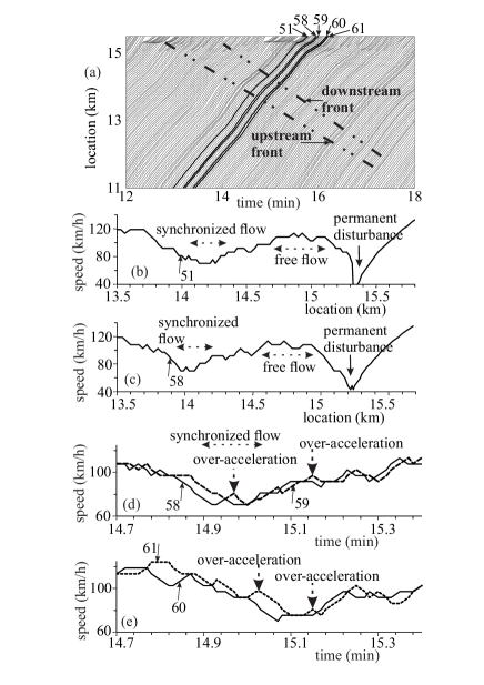
Figure 16: Simulations of over-acceleration effect that leads to S$\rightarrow$F instability, i.e., to the growing speed wave of increase in speed within synchronized flow at on-ramp bottleneck: (a) Fragment of vehicle trajectories in space and time related to Fig. 12 (b–d). (b–e) Microscopic vehicle speeds along trajectories as road location-functions (b, c) and time-functions (d, e) labeled by the same numbers as those in (a).

We have found that during the time delay of traffic breakdown $0<t<T^{\rm(B)}_{1}$ (Figs. 10 (a) and 12 (a)) there is a permanent spatiotemporal competition between the speed adaptation effect supporting an F$\rightarrow$S transition and the over-acceleration effect supporting an S$\rightarrow$F instability that counteracts the emergence of synchronized flow. This competition results in the occurrence of a permanent speed decrease in a neighborhood of the bottleneck that we call $``$permanent speed disturbance” at the bottleneck. There can be distinguished two cases of this competition:

(i) There is a noticeable time lag between the beginning of an F$\rightarrow$S transition due to the speed adaptation and the beginning of an S$\rightarrow$F instability due to over-acceleration that prevents the formation of a congested pattern at the bottleneck; this case we call $``$a sequence of F$\rightarrow$S$\rightarrow$F transitions” at the bottleneck.

(ii) There is a spatiotemporal $``$overlapping” of the speed adaptation and over-acceleration effects (Sec. IV.3).

One of the sequences of F$\rightarrow$S$\rightarrow$F transitions within the permanent speed disturbance at on-ramp bottleneck is marked by dashed-dotted curves in Fig. 12 (a, c). An F$\rightarrow$S transition and a return S$\rightarrow$F transition that build the sequence of F$\rightarrow$S$\rightarrow$F transitions are explained as follows (Figs. 12 (b–e)–16).

IV.2.1 F$\rightarrow$S transition

After several slow moving vehicles have merged from the on-ramp onto the main road (bold dotted vehicle trajectories in Fig. 13 (a)), the following vehicles on the main road have to decelerate strongly due to the speed adaptation effect (vehicle trajectories 42 and 43 in Fig. 13 (a–c)). This results in the upstream propagation of synchronized flow upstream of the bottleneck, i.e., an F$\rightarrow$S transition occurs (vehicle trajectories 42–46 in Fig. 13 (a–f)). Microscopic features of this F$\rightarrow$S transition (in particular, the upstream propagation of the upstream front of synchronized flow labeled by $``$front of F$\rightarrow$S transition” in Fig. 12 (a)) are qualitatively the same as those shown in Fig. 11.

Moreover, after the F$\rightarrow$S transition has occurred, in synchronized flow that has emerged at the bottleneck speed peaks appear (speed peaks 1 and 2 in Fig. 14 (b, d)) (see item (iii) of the common microscopic features of traffic breakdown of Sec. IV.1). The physics of the speed peaks is the same as that discussed in Secs. II.2 and III.1. The speed peaks lead to the emergence of dissolving speed waves in the synchronized flow (Fig. 14); the dissolving waves have also qualitatively the same microscopic features as shown in Fig. 9.

IV.2.2 Return S$\rightarrow$F transition due to S$\rightarrow$F instability

A crucial difference of the case under consideration (Fig. 12) with traffic breakdown shown in Fig. 11 becomes clear when we consider Fig. 15. We find that synchronized flow exists for a few minutes only: A speed peak (speed peak 3 in Fig. 15) occurs at the downstream front of this synchronized flow that initiates an S$\rightarrow$F instability at the bottleneck. The S$\rightarrow$F instability interrupts the formation of a congested pattern at the bottleneck.

Indeed, due to the S$\rightarrow$F instability, rather than an WSP occurs, as this is realized in Fig. 11, a localized region of synchronized flow departs from the bottleneck: The downstream front and the upstream front of this synchronized flow (labeled by $``$downstream front” and $``$upstream front” in Figs. 12 (c, d) and 16 (a)) propagate upstream from the bottleneck. While propagating upstream from the bottleneck, synchronized flow dissolves over time. Due to the occurrence of such a dissolving synchronized flow, the minimum speed $v_{\rm min}(t)$ within the permanent disturbance firstly decreases and then increases over time (trajectories 32–41 in Fig. 12 (e)).

The physics of the S$\rightarrow$F instability is the same as disclosed in Sec. II.3. In particular, the S$\rightarrow$F instability leads to a growing wave of increase in speed within synchronized flow (labeled by $``$growing speed wave” in Fig. 15). The growth of the speed wave is realized due to over-acceleration effect (Fig. 16) whose physics is the same as that discussed in Sec. II.3.

IV.3 Spatiotemporal $``$overlapping” speed adaptation and over-acceleration effects

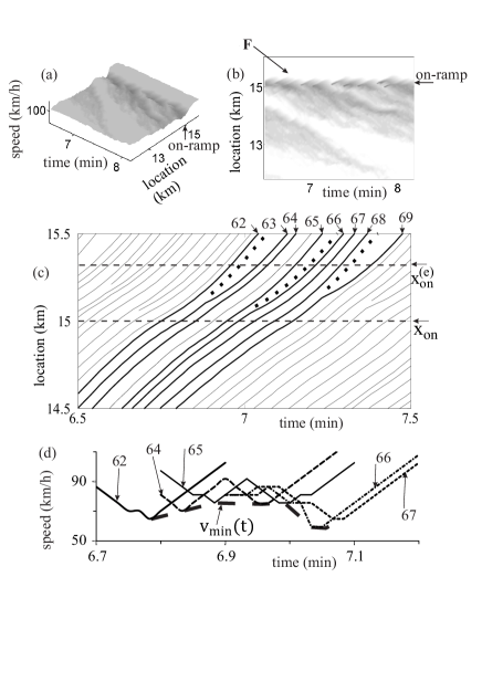
Figure 17: Simulations of dynamics of permanent disturbance at on-ramp bottleneck: (a, b) Speed in space and time (a) and the same speed data presented by regions with variable shades of gray (in white regions the speed is equal to or higher than 100 km/h, in black regions the speed is equal to 20 km/h) (b) for a short time interval related to $t<T^{\rm(B)}_{1}$ in Fig. 10 (a). (c) Fragment of vehicle trajectories in space and time. (d) Microscopic vehicle speeds along trajectories as time functions labeled by the same numbers as those in (c).

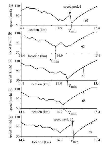
Figure 18: Simulations of the occurrence of speed peaks and their evolution within a permanent disturbance at on-ramp bottleneck: (a–e) Microscopic vehicle speeds along trajectories as road location-functions labeled by the same numbers as those in Fig. 17 (c).

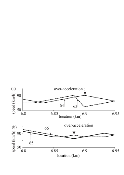
Figure 19: Simulations of over-acceleration within a permanent disturbance at on-ramp bottleneck: (a, b) Microscopic vehicle speeds along trajectories as road location-functions labeled by the same numbers as those in Fig. 17 (c).

During time delay $0<t<T^{\rm(B)}_{1}$ of the breakdown (Fig. 10 (a)), there are also time intervals within which there is no noticeable time lag between the beginning of the F$\rightarrow$S transition and the S$\rightarrow$F instability due to over-acceleration. In this case, rather than to distinguish a sequence of F$\rightarrow$S$\rightarrow$F transitions within the permanent speed disturbance at the bottleneck, we find a spatiotemporal $``$overlapping” of the speed adaptation and over-acceleration effects.

In this case (Figs. 17–19), there is an upstream front of the permanent disturbance within which vehicles on the main road decelerate to a smaller speed due to slower moving vehicles that merge from the on-ramp. Vehicles upstream of the upstream front of the disturbance move at their maximum free flow speed $v_{\rm free}$. There is also a downstream front of the disturbance within which vehicles accelerate to the maximum free flow speed $v_{\rm free}$ (Fig. 17). We have found that the distribution of the speed within the permanent disturbance exhibits a complex spatiotemporal dynamics:

(i) The value of the minimum speed $v_{\rm min}$ within the disturbance changes randomly over time (Fig. 17 (d)).

(ii) This speed minimum occurs randomly at different road locations (Fig. 18).

(iii) There can be several speed maxima within the disturbance whose locations are also change randomly (Fig. 18).

This complex dynamics of the permanent speed disturbance at the bottleneck is explained as follows. As in the fully developed synchronized flow (Fig. 8 (a)), within the permanent speed disturbance there is a sequence of speed peaks that occur randomly at the downstream front of the permanent speed disturbance (labeled by $``$speed peak 1” and $``$speed peak 2” in Fig. 18 (a, c)). The physics of these speed peaks is the same as that already explained in Sec. II.2.

Due to the speed peaks, regions of increase in speed appears propagating upstream within the disturbance. Within the regions of speed increase, the over-acceleration effect occurs that prevents the upstream propagation of the upstream front of synchronized flow due to the speed adaptation. Examples of the over-acceleration effect are shown in Fig. 19. Vehicle 63 accelerates firstly and then begins to decelerates strongly (Fig. 19 (a); see also speed peak 1 shown in Fig. 18 (a)). However, the following vehicle 64 continues to accelerate even when preceding vehicle 63 decelerates strongly (labeled by $``$over-aceleration” in (Fig. 19 (a))). In another example, the following vehicle 66 begins to accelerate when the preceding vehicle 65 starts to decelerate (labeled by $``$over-aceleration” in (Fig. 19 (b))).

These over-acceleration effects can be considered short time S$\rightarrow$F instabilities that increase the speed within the permanent speed disturbance. These short time S$\rightarrow$F instabilities prevent a continuous propagation of the upstream front of the permanent speed disturbance, i.e., they prevent traffic breakdown at the bottleneck. Therefore, rather than traffic breakdown (Fig. 11 (a, d)) resulting in the formation of ${\rm WSP_{1}}$ (Fig. 10 (a)), the permanent speed disturbance persists at the bottleneck (Fig. 17 (a, d)). Thus, the competition between speed adaptation and over-acceleration determines a random time delay of traffic breakdown at the bottleneck independent on whether sequences of F$\rightarrow$S$\rightarrow$F transitions (Sec. IV.2) can be distinguished or not within the permanent speed disturbance at the bottleneck.

V General character of effect of S$\rightarrow$F instability on nucleation nature of traffic breakdown

In Sec. IV, we have found that an S$\rightarrow$F instability is the origin of sequences of F$\rightarrow$S$\rightarrow$F transitions at the bottleneck. In its turn, the F$\rightarrow$S$\rightarrow$F transitions is the reason of the nucleation nature of traffic breakdown. In other words, the S$\rightarrow$F instability governs the nucleation character of traffic breakdown at the bottleneck.

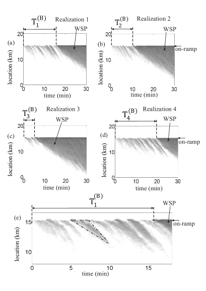
Figure 20: Random time delay of traffic breakdown (F$\rightarrow$S transition) at on-ramp bottleneck at a larger on-ramp inflow rate $q_{\rm on}=$ 480 vehicles/h than that in Fig. 10: (a–d) Speed in space and time for four different simulation realizations (runs) presented by regions with variable shades of gray (in white regions the speed is equal to or higher than 110 km/h, in black regions the speed is zero). (e) Speed in space and time presented by regions with variable shades of gray illustrating F$\rightarrow$S$\rightarrow$F transitions during time delay of traffic breakdown related to realization 1 in (a). Time delays of traffic breakdown $T^{\rm(B)}$ in different simulation realizations 1–4 are $T^{\rm(B)}_{1}=$ 16 min (a), $T^{\rm(B)}_{2}=$ 11 min (b), $T^{\rm(B)}_{3}=$ 6 min (c), and $T^{\rm(B)}_{4}=$ 20 min (d). The flow rate in free flow upstream of the bottleneck is the same as that in Fig. 10: $q_{\rm in}=$ 1406 vehicles/h.

However, when the on-ramp inflow rate $q_{\rm on}$ increases considerably, no S$\rightarrow$F instability is observed within congested patterns (WSPs) that emerge after traffic breakdown has occurred at the bottleneck (Fig. 20 (a–d)) General . This is in contrast with the WSPs shown in Fig. 10.

Due to the increase in $q_{\rm on}$, the mean speed of synchronized flow in WSPs shown in Fig. 20 (a–d) that emerge at the bottleneck after traffic breakdown has occurred becomes smaller than the mean speed of synchronized flow in WSPs shown in Fig. 10 (a, c). We have found that also in the case of the WSPs shown in Fig. 20 (a–d) there are many random speed peaks at the downstream front of synchronized flow; the speed peaks (not shown) are qualitatively the same as those in Fig. 8. However, due to a smaller mean speed of synchronized flow in the WSPs, no S$\rightarrow$F instability can be initiated by these speed peaks during the whole time of the observation of traffic flow $T_{\rm ob}=$ 30 min in Fig. 20: The speed peaks initiate only dissolving speed waves in synchronized flow (not shown) that are qualitatively similar to those shown in Figs. 8 (b) and 9 found for a smaller on-ramp inflow rate.

Although there are no S$\rightarrow$F instabilities within the WSPs, we have found random time delays of traffic breakdown at the bottleneck (Fig. 20 (a–d)) that exhibit the same features as those in Fig. 10 (a–d). We have also found that there are sequences of F$\rightarrow$S$\rightarrow$F transitions that are the reason for the existence of a random time delay of traffic breakdown. Each of the sequences of F$\rightarrow$S$\rightarrow$F transitions (one of them is marked by dashed-dotted curves in Fig. 20 (e)) exhibits qualitatively the same physical features as those found out in Sec. IV.2.

In other words, the result of this article that the S$\rightarrow$F instability governs the metastability of free flow with respect to traffic breakdown at the bottleneck exhibits a general character. The physics of this general result is as follows.

(i) There are sequences of F$\rightarrow$S$\rightarrow$F transitions at the bottleneck (Sec. IV.2). On average, the F$\rightarrow$S$\rightarrow$F transitions cause a permanent speed disturbance, i.e., a permanent decrease in speed in free flow localized at the bottleneck. The permanent speed disturbance exhibits a complex dynamic behavior in space and time.

(ii) When a decrease in speed within the permanent speed disturbance in free flow becomes randomly equal to or larger than some critical decrease in speed, the resulting F$\rightarrow$S transition, i.e., the upstream propagation of the upstream front of the synchronized flow cannot be suppressed by the S$\rightarrow$F instability. In this case as considered in Sec. IV.1, rather than a sequence of F$\rightarrow$S$\rightarrow$F transitions, a congested pattern emerges at the bottleneck (WSPs in Figs. 10 and 20). Otherwise, when the local decrease in speed in free flow at the bottleneck is smaller than the critical one, the S$\rightarrow$F instability interrupts the development of the F$\rightarrow$S transition: Rather than the congested pattern, a sequence of the F$\rightarrow$S$\rightarrow$F transitions occurs at the bottleneck.

(iii) There can be a time interval during which any decrease in speed within the permanent speed disturbance in free flow at the bottleneck is smaller than the critical one. In this case, the S$\rightarrow$F instability interrupts the development of each of the F$\rightarrow$S transitions. This time interval is the time delay $T^{\rm(B)}$ of traffic breakdown (Figs. 10 and 20).

(iv) The time delay of traffic breakdown (Figs. 10 and 20 (a–d)) is a random value because the S$\rightarrow$F instability exhibits the nucleation nature: The S$\rightarrow$F instability occurs only if a large enough initial increase in speed, which is equal to or larger than a critical increase in speed, appears randomly within the emergent synchronized flow at the bottleneck.

(v) The critical increase in speed in synchronized flow, at which an S$\rightarrow$F instability occurs, depends on the critical decrease in speed within the permanent speed disturbance in free flow at the bottleneck, at which traffic breakdown occurs: When the S$\rightarrow$F instability cannot interrupt the development of the F$\rightarrow$S transition, a congested pattern is formed at the bottleneck.

If the on-ramp inflow rate $q_{\rm on}$ increases, while the flow rate on the main road upstream of the bottleneck $q_{\rm in}$ remains, we have found the following effects:

1. Within synchronized flow of a congested pattern at the bottleneck, the probability of the occurrence of the S$\rightarrow$F instability decreases. Indeed, in contrast with the cases shown in Figs. 10 (a–d), there is no S$\rightarrow$F instability within WSPs in Figs. 20 (a–d).

2. The mean time delay of traffic breakdown becomes shorter: The mean value of the time delay of traffic breakdowns shown in Fig. 20 is shorter than that in Fig. 10.

VI Discussion

VI.1 Classical traffic flow instability versus S$\rightarrow$F instability of three-phase theory

The basic difference between the classical traffic flow instability GH195910 ; Gazis1961A10 ; GH10 ; Chandler ; KS ; KS1959A ; Newell1961 ; Newell1963A ; Newell1981 ; Newell_Stoch ; Gipps ; Gipps1986 ; Wiedemann ; Whitham1990 ; ach_Pay197110 ; ach_Pay197910 ; Stoc ; Bando1995 ; ach_Kra10 ; fail_Nagatani1998A ; fail_Nagatani1999B ; ach_Helbing200010 ; ach_Aw200010 ; ach_Jiang2001A ; Reviews ; Reviews2 and an S$\rightarrow$F instability of three-phase theory is as follows: The classical traffic instability is a growing wave of local decrease in speed in free flow (Fig. 21 (a)) GH195910 ; Gazis1961A10 ; GH10 ; Chandler ; KS ; KS1959A ; Newell1961 ; Newell1963A ; Newell1981 ; Newell_Stoch ; Gipps ; Gipps1986 ; Wiedemann ; Whitham1990 ; ach_Pay197110 ; ach_Pay197910 ; Stoc ; Bando1995 ; ach_Kra10 ; fail_Nagatani1998A ; fail_Nagatani1999B ; ach_Helbing200010 ; ach_Aw200010 ; ach_Jiang2001A ; Reviews ; Reviews2 . Contrary, the S$\rightarrow$F instability is a growing wave of local increase in speed in synchronized flow (Fig. 21 (b, c)).

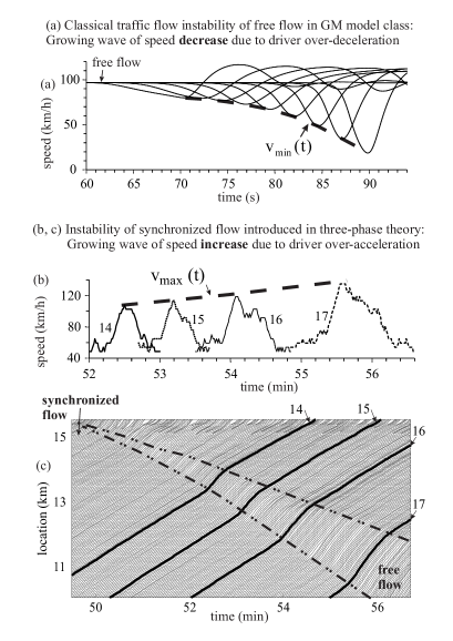
Figure 21: Classical traffic flow instability (a) GH195910 ; Gazis1961A10 ; GH10 ; Chandler ; KS ; KS1959A ; Newell1961 ; Newell1963A ; Newell1981 ; Newell_Stoch ; Gipps ; Gipps1986 ; Wiedemann ; Whitham1990 ; ach_Pay197110 ; ach_Pay197910 ; Stoc ; Bando1995 ; ach_Kra10 ; fail_Nagatani1998A ; fail_Nagatani1999B ; ach_Helbing200010 ; ach_Aw200010 ; ach_Jiang2001A ; Reviews ; Reviews2 versus S$\rightarrow$F instability of three-phase theory (b, c): (a) Vehicle trajectories as time-functions showing the well-known growing wave of speed reduction caused by classical traffic flow instability with simulations of optimal velocity model by Bando et al. Bando1995 ; Bando_Model . (b, c) Vehicle trajectories as time-functions (b) (taken from Fig. 7) and in space and time showing the growing wave of speed increase caused by S$\rightarrow$F instability (taken from Fig. 3).

The classical traffic flow instability GH195910 ; Gazis1961A10 ; GH10 ; Chandler ; KS ; KS1959A ; Newell1961 ; Newell1963A ; Newell1981 ; Newell_Stoch ; Gipps ; Gipps1986 ; Wiedemann ; Whitham1990 ; ach_Pay197110 ; ach_Pay197910 ; Stoc ; Bando1995 ; ach_Kra10 ; fail_Nagatani1998A ; fail_Nagatani1999B ; ach_Helbing200010 ; ach_Aw200010 ; ach_Jiang2001A ; Reviews ; Reviews2 should explain traffic breakdown through the driver reaction time (time delay in driver over-deceleration). However, this classical traffic flow instability leads to a phase transition from free flow to a wide moving jam (F$\rightarrow$J transition) KK1993 ; Reviews2 ; Kerner_Review ; KernerBook ; KernerBook2 . The classical instability has been incorporated in a huge number of traffic flow models Reviews2 ; Kerner_Review . Contrary to the classical traffic flow instability, in real field traffic data, traffic breakdown is an F$\rightarrow$S transition. A more detailed explanation why the classical traffic flow instability have failed to explain real traffic breakdown can be found in Kerner_Review .

However, it should be noted that the classical traffic instability GH195910 ; Gazis1961A10 ; GH10 ; Chandler ; KS ; KS1959A ; Newell1961 ; Newell1963A ; Newell1981 ; Newell_Stoch ; Gipps ; Gipps1986 ; Wiedemann ; Whitham1990 ; ach_Pay197110 ; ach_Pay197910 ; Stoc ; Bando1995 ; ach_Kra10 ; fail_Nagatani1998A ; fail_Nagatani1999B ; ach_Helbing200010 ; ach_Aw200010 ; ach_Jiang2001A ; Reviews ; Reviews2 has also been used in three-phase theory to explain a growing wave of local decrease in speed within synchronized flow leading to the emergence of a wide moving jam(s) in synchronized flow (S$\rightarrow$J transition) (Fig. 1 (d)) Kerner1998B ; KernerBook . Thus in three-phase theory, the emergence of wide moving jams is realized through a sequence of F$\rightarrow$S$\rightarrow$J transitions Kerner1998B ; KernerBook .

VI.2 Traffic breakdown without over-acceleration

Figure 22: Simulations of traffic breakdown at on-ramp bottleneck with the KKSW CA model in which either the probability of over-acceleration $p_{\rm a}=0$ (a–e) (Sec. VI.2) or the probability of over-acceleration $p_{\rm a}=1$ (f) (Sec. VI.3): (a, c, e, f) Speed in space and time presented by regions with variable shades of gray (in white regions the speed is equal to or higher than 130 km/h (a, c) or 120 km/h (e, f), in black regions the speed is equal to 30 km/h (a, c) or zero (e, f)). (b, d) Microscopic vehicle speeds along one of the vehicle trajectories moving within patterns in (a, c), respectively. $q_{\rm on}=$ 360 (a–d, f) and 900 (e) vehicles/h, $q_{\rm in}=$ 1800 (f), 1406 (a, b, e), and 1125 vehicles/h (c, d). Other model parameters are the same as those given in caption to Fig. 2.

When in (II.1.1) the probability of over-acceleration $p_{\rm a}=0$, there is no over-acceleration in the KKSW CA model. In this case, no S$\rightarrow$F instability is realized. For this reason, we find that congested traffic emerges at the bottleneck without any delay. The downstream front of the pattern is fixed at the bottleneck (Fig. 22 (a, b)). When we decrease the flow rate on the main road, congested traffic occurs also without any time delay; due to smaller flow rate upstream, the upstream front of this congested traffic propagates slower only (Fig. 22 (c, d)). Because the downstream front of the congested traffic is fixed at the bottleneck we can call it as $``$synchronized flow”.

In other words, features of the synchronized flow shown in Fig. 22 (a–d) contradict the nucleation nature of traffic breakdown (F$\rightarrow$S transition) found in real field traffic data. Thus over-acceleration is needed to simulate the nucleation nature of an F$\rightarrow$S transition of real traffic.

The absent of over-acceleration ($p_{\rm a}=0$) does not affect the slow-of-start rule used in the KKSW CA model. Therefore, we can expect that an S$\rightarrow$J instability can occur within synchronized flow leading to the emergence of a wide moving jam(s). Indeed, when we increase the on-ramp inflow rate, so that the mean speed in synchronized flow decreases considerably, moving jams emerge in this dense synchronized flow (Fig. 22 (e)).

VI.3 Traffic breakdown without time delay of over-acceleration

The necessity of the existence of a finite time delay in over-acceleration to simulate an S$\rightarrow$F instability and, therefore, the nucleation features of traffic breakdown becomes more clear, if we assume that over-acceleration occurs with probability $p_{\rm a}=$1, i.e., without any time delay.

Because such a limit case is not attained with the KKSW CA model (II.1.1)–(12), we should make the following changes in the model: When $p_{\rm a}=$1, model step (c) (Eq. (II.1.1)) is satisfied with probability 1. In step (f) (Eq. (7)), rather than Eq. (10), the following formula is used

$$r<p.$$ (19)

We have found that when over-acceleration occurs without time delay, such over-acceleration prevents speed adaptation within 2D-states of synchronized flow. Therefore, synchronized flow states are not realized. In other words, there are no S$\rightarrow$F instability and no time-delayed F$\rightarrow$S transition in this model. In general, such model exhibits qualitatively the same features of traffic breakdown at the bottleneck as those of the NaSch CA model Stoc2 ; Schadschneider_Book : Traffic breakdown is governed by the classical traffic flow instability of the GM model class (Sec. VI.1) leading to a well-known time-delayed F$\rightarrow$J transition (Fig. 22 (f)).

VI.4 General microscopic features of the S$\rightarrow$F instability

Microscopic features of the S$\rightarrow$F instability derived above based on a study of the KKSW CA model exhibit general character, i.e., they are independent on specific properties of the KKSW CA model. To prove this statement, we show that qualitatively the same features of the S$\rightarrow$F instability can be derived with simulations of the Kerner-Klenov stochastic three-phase model of KKl ; KKl2003A ; KKl2009A . We use a discrete in space model version of KKl2009A for a single lane road with an on-ramp bottleneck (Appendix A).

VI.4.1 Nucleation features of S$\rightarrow$F instability

(i) As in Fig. 3 (a, b), after traffic breakdown (F$\rightarrow$S transition) has occurred at the bottleneck, synchronized flow emerges whose downstream front is localized at the bottleneck (Fig. 23 (a, b)). A random sequence of speed peaks appears at the downstream front of synchronized flow at the bottleneck (Fig. 23 (c); compare with Fig. 8 (a)). The speed peaks are disturbances of increase in speed in synchronized flow within which the microscopic (single-vehicle) speed is higher than the average synchronized flow speed (Fig. 23 (d, e); compare with Figs. 4 (b) and 8 (c)).

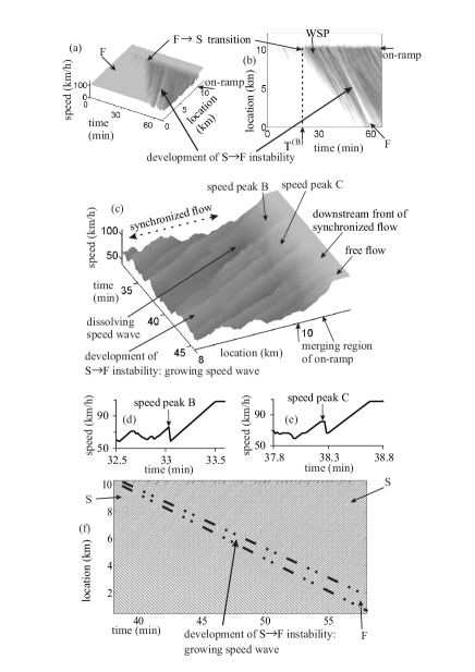
Figure 23: Simulations of speed peaks at downstream front of synchronized flow and S$\rightarrow$F instability at on-ramp bottleneck on single-lane road with the Kerner-Klenov model (Tables 1–5 of Appendix A): (a, b) Speed in space and time (a) and the same data presented by regions with variable shades of gray (in white regions the speed is equal to or higher than 100 km/h, in black regions the speed is zero) (b). (c) Speed in space and time for time $t>T^{\rm(B)}$ within synchronized flow of WSP; two of the speed peaks in (c) are marked by $``$speed peak B” and $``$speed peak C”. (d, e) Microscopic (single-vehicle) speeds along vehicle trajectories as time-functions showing speed peak B (d) leading to a dissolving speed wave (labeled by $``$dissolving speed wave” in (b)) and speed peak C (e) initiating a growing speed wave (labeled by $``$development of S$\rightarrow$F instability: growing speed wave” in (b)). The physics of speed peaks B and C is the same as that for speed peaks shown in Figs. 8 (a, c) and 4 (b): vehicles shown in (d, e), which begin to accelerate at the downstream front of synchronized flow, have to interrupt their acceleration and to decelerate due to vehicles merging from the on-ramp onto the main road. $x_{\rm on}=$ 10 km and $x^{\rm(e)}_{\rm on}=10.3$ km are, respectively, the beginning and the end of the merging region of the on-ramp. (f) Fragment of vehicle trajectories in space and time related to (a, b) (each 5th vehicle is shown); bold dashed-dotted curves in (f) mark the development of S$\rightarrow$F instability in synchronized flow. F – free flow, S – synchronized flow, WSP – widening synchronized flow pattern. $q_{\rm on}=$ 170 vehicles/h, $q_{\rm in}=$ 2278 vehicles/h. Other model parameters are given in Tables 6 and 7.

(ii) As in Fig. 8 (b), small speed peaks (small disturbances of increase in speed) in synchronized flow lead to dissolving speed waves of increase in speed in synchronized flow ($``$dissolving speed wave” in Fig. 23 (c)). In this case, no S$\rightarrow$F instability occurs.

(iii) Only when a speed peak with a large enough increase in speed occurs randomly at the downstream front of synchronized flow at the bottleneck, the speed peak initiates the S$\rightarrow$F instability: A growing speed wave of increase in speed occurs in synchronized flow whose growth leads to an S$\rightarrow$F transition ($``$growing speed wave” in Fig. 23 (c, f); compare with Fig. 3 (e)). As shown with simulations of the KKSW CA model in Fig. 6, simulations with the Kerner-Klenov model confirm (not shown) that the S$\rightarrow$F instability occurs due to the over-acceleration effect.

The behavior of disturbances of increase in speed in synchronized flow (items (ii) and (iii)) proves the nucleation nature of the S$\rightarrow$F instability.

VI.4.2 S$\rightarrow$F instability as origin of nucleation nature of traffic breakdown at highway bottlenecks

As found in Secs. IV and V based on simulations with the KKSW CA model, simulations with the Kerner-Klenov model show also that an S$\rightarrow$F instability tries to prevent an F$\rightarrow$S transition in free flow at the bottleneck as follows (Figs. 24 and 25).

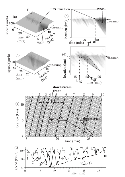
Figure 24: Simulations of F$\rightarrow$S$\rightarrow$F transitions within a permanent speed disturbance at on-ramp bottleneck on single-lane road with the Kerner-Klenov model (Tables 1–5 of Appendix A): (a, b) Speed in space and time (a) and the same data presented by regions with variable shades of gray (in white regions the speed is equal to or higher than 105 km/h, in black regions the speed is equal to 0 km/h). (c, d) Speed in space and time (c) and the same data presented by regions with variable shades of gray (d) (in white regions the speed is equal to or higher than 100 km/h, in black regions the speed is equal to 20 km/h) for a short time interval in (a, b). (e) Fragment of vehicle trajectories in space and time related to (c, d). (f) Microscopic vehicle speeds along trajectories as time functions labeled by the same numbers as those in (e). In (d, e), dashed-dotted lines mark emergent synchronized flow that dissolves due to S$\rightarrow$F instability (labels $``$downstream front” and $``$upstream front” show boundaries of the synchronized flow region). F – free flow, WSP – widening synchronized flow pattern. $q_{\rm on}=$ 320 vehicles/h, $q_{\rm in}=$ 2000 vehicles/h. Other model parameters are given in Tables 6 and 7.

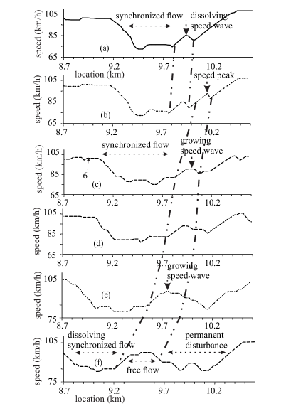
Figure 25: Microscopic vehicle speeds as road location-functions related to Fig. 24 (e): Some of the vehicles moving at different times (that increase from (a) to (f), respectively, within a time interval between vehicles 5 and 8 shown in Fig. 24 (e)) propagate through the emergent synchronized flow that is marked by dashed-dotted lines in Fig. 24 (d, e). Dissolving and growing speed waves of increase in speed within the emergent synchronized flow are marked by bold dashed-dotted curves labeled by $``$dissolving speed wave” and $``$growing speed wave”, respectively. Vehicle 6 in (c) is the same as vehicle 6 marked in Fig. 24 (e).

(i) When the on-ramp inflow $q_{\rm on}$ is switched on ($t>0$ in Fig. 24 (a, b)), vehicles that merge from the on-ramp onto the main road cause a speed disturbance of decrease in speed in free flow on the main road in a neighborhood of the bottleneck. The following vehicles have to decelerate while adapting their speed a smaller speed within the disturbance. Due to this speed adaptation effect, synchronized flow emerges on the main road upstream at the bottleneck. See an example of the beginning of a such F$\rightarrow$S transition at time instant $t_{\rm FS}$ in Fig. 24 (d). The mean speed in this emergent synchronized flow is the smaller, the larger the initial speed disturbance of decrease in speed in free flow.

(ii) Within the downstream front of the emergent synchronized flow, speed peaks appear. Small speed peaks cause dissolving waves of increase in speed in the synchronized flow ($``$dissolving speed wave” in Fig. 25 (a, b)). When a large enough speed peak occurs, the peak initiates a growing wave of increase in speed within the synchronized flow ($``$growing speed wave” in Fig. 25 (b–f)): At a time instant (labeled by $t_{\rm SF}$ in Fig. 24 (d)) an S$\rightarrow$F instability is realized at the bottleneck. This S$\rightarrow$F instability destroys the emergent synchronized flow. As a result, the region of synchronized flow dissolves and free flow recovers at the bottleneck. In accordance with Sec. IV.2, the sequence of the emergence of the synchronized flow (the beginning of an F$\rightarrow$S transition) with the subsequent S$\rightarrow$F instability can be considered F$\rightarrow$S$\rightarrow$F transitions at the bottleneck (Fig. 24 (c–f); compare with Fig. 12 (b–e)). Due to many sequences of F$\rightarrow$S$\rightarrow$F transitions, local permanent speed disturbance is realized in free flow at the bottleneck (time interval $0<t<T^{\rm(B)}$ in Fig. 24 (a, b); compare with Fig. 12 (a)).

(iii) As long as F$\rightarrow$S$\rightarrow$F transitions occur, no traffic breakdown (F$\rightarrow$S transition) with the subsequent formation of congested pattern is realized at the bottleneck (time interval $0<t<T^{\rm(B)}$ in Fig. 24 (a, b); compare with Fig. 12 (a)) during time interval $0<t<T^{\rm(B)}_{1}$).

(iv) The S$\rightarrow$F instability exhibits the nucleation nature. Therefore, there can be a random time instant $t=T^{\rm(B)}$ at which no S$\rightarrow$F instability occurs that can prevent the development of an F$\rightarrow$S transition. In this case, the F$\rightarrow$S transition leads to the formation of the congested pattern (WSP in Fig. 24 (a, b) at $t>T^{\rm(B)}$; compare with Fig. 12 (a) at $t>T^{\rm(B)}_{1}$).

Thus as simulations with the KKSW CA model (Secs. II–V), simulations with the Kerner-Klenov model (Figs. 23–24) prove that small disturbances of decrease in speed in free flow at the bottleneck are destroyed through the S$\rightarrow$F instability. In contrast, great enough disturbances of decrease in speed in free flow cannot be destroyed resulting in an F$\rightarrow$S transition with the formation of the congested pattern at the bottleneck. This explains why through the nucleation character of the S$\rightarrow$F instability caused by the over-acceleration effect, free flow at the bottleneck is in a metastable state with respect to the F$\rightarrow$S transition and there is a random time delay $T^{\rm(B)}$ to this F$\rightarrow$S transition.

VI.5 Conclusions

The S$\rightarrow$F instability exhibits the following general microscopic features, which are qualitatively identical ones in simulations with the KKSW CA and Kerner-Klenov stochastic traffic flow models in the framework of the three-phase theory.

VI.5.1 Summary of nucleation features of S$\rightarrow$F instability

(i) An initial speed disturbance of increase in speed within synchronized flow (S) at the bottleneck can transform into a growing speed wave of increase in speed (growing acceleration wave) that propagates upstream within synchronized flow and leads to free flow (F) at the bottleneck. This S$\rightarrow$F instability is caused by the over-acceleration effect.

(ii) The S$\rightarrow$F instability can occur, if there is a finite time delay in over-acceleration.

(iii) Due to the S$\rightarrow$F instability, the downstream front of the initial synchronized flow begins to move upstream from the bottleneck, while free flow appears at the bottleneck.

(iv) In simulations, the initial speed disturbance of increase in speed that initiates the S$\rightarrow$F instability at the bottleneck occurs at the downstream front of synchronized flow. We call the initial speed disturbance as $``$speed peak”.

(v) There can be many speed peaks with random amplitudes that occur randomly over time at the downstream front of synchronized flow. Only when a large enough speed peak appears, the S$\rightarrow$F instability occurs. Speed peaks of smaller amplitude cause dissolving speed waves of increase in speed (dissolving acceleration waves) in synchronized flow: All these waves dissolve over time while propagating upstream within synchronized flow. As a result, the synchronized flow persists at the bottleneck. Thus, the S$\rightarrow$F instability exhibits the nucleation nature.

VI.5.2 S$\rightarrow$F instability as origin of nucleation nature of traffic breakdown

The S$\rightarrow$F instability in synchronized flow at the bottleneck governs traffic breakdown (i.e., F$\rightarrow$S transition) resulting in the formation of a congested pattern at the bottleneck as follows.

(i) A sequence of F$\rightarrow$S$\rightarrow$F transitions that interrupts the formation of a congested pattern at the bottleneck. When an F$\rightarrow$S transition begins to develop, i.e., the upstream front of synchronized flow begins to propagate upstream from the bottleneck, an S$\rightarrow$F instability can randomly occur. Due to the S$\rightarrow$F instability, free flow appears at the bottleneck. As a result, the downstream front of the synchronized flow departs upstream from the bottleneck. In its turn, this results in the dissolution of the synchronized flow, i.e., in the interruption of the formation of a congested pattern due to the F$\rightarrow$S transition. We call this effect as the sequence of F$\rightarrow$S$\rightarrow$F transitions.

(ii) Metastability of free flow with respect to traffic breakdown (F$\rightarrow$S transition) and a random time delay to traffic breakdown. There can be many sequences of F$\rightarrow$S$\rightarrow$F transitions. Each of them interrupts the formation of a congested pattern at the bottleneck. This explains the existence of a time delay of traffic breakdown: Rather than the congested pattern appears at the bottleneck, the sequences of F$\rightarrow$S$\rightarrow$F transitions result in a narrow region of decrease in speed in free flow localized at the bottleneck (called as a $``$permanent speed disturbance” in free flow at the bottleneck). The time delay of traffic breakdown (F$\rightarrow$S transition) $T^{\rm(B)}$ is a random value: There can be a time instant $T^{\rm(B)}$ at which, after an F$\rightarrow$S transition begins to develop, there is no S$\rightarrow$F instability that can prevent the subsequent development of the F$\rightarrow$S transition. This F$\rightarrow$S transition leads to the formation of a congested pattern at the bottleneck.

Microscopic qualitative features of the S$\rightarrow$F instability exhibit general character: These features are independent on specific properties of a stochastic traffic flow model that incorporates hypotheses of the three-phase theory.

An empirical evidence of S$\rightarrow$F transitions at highway bottlenecks have been proven in Kerner2002A . However, real field traffic data studied in Kerner2002A (as well as in all other publications known to the author) are macroscopic traffic data. To prove the microscopic theory developed in this article with real field traffic data, measurements of microscopic (single-vehicle) spatiotemporal data (e.g., vehicle trajectories) of almost all vehicles moving in free and synchronized flows in a neighborhood of a highway bottleneck are required. Unfortunately, such empirical microscopic traffic data is not currently available. Therefore, a microscopic empirical study of traffic flow will be a very interesting task for further investigations of traffic flow.

Appendix A Kerner-Klenov model for single-lane road with on-ramp bottleneck

In this Appendix, we present a discrete version of the Kerner-Klenov stochastic three-phase traffic flow model for single-lane road with on-ramp bottleneck KKl2009A used in simulations shown in Figs. 23–25 (Sec. VI.4). In the model (Tables 1–5), index $n$ corresponds to the discrete time $t_{\rm n}=\tau n,\ n=0,1,...$, $v_{n}$ is the vehicle speed at time step $n$, $a$ is the maximum acceleration, $\tilde{v}_{n}$ is the vehicle speed without speed fluctuations $\xi_{n}$, the lower index $\ell$ marks variables related to the preceding vehicle, $v_{{\rm s},n}$ is a safe speed at time step $n$, $v_{\rm free}$ is the maximum speed in free flow, $\xi_{n}$ describes speed fluctuations; $v_{{\rm c},n}$ is a desired speed; all vehicles have the same length $d$ that includes the mean space gap between vehicles within a wide moving jam where the speed is zero. In the model, discretized space coordinate with a small enough value of the discretization cell $\delta x$ is used. Consequently, the vehicle speed and acceleration discretization intervals are $\delta v=\delta x/\tau$ and $\delta a=\delta v/\tau$, respectively. In the model of an on-ramp bottleneck (Table 5; see explanations of model parameters in Fig. 16.2 (a) of KernerBook ), superscripts $+$ and $-$ in variables, parameters, and functions denote the preceding vehicle and the trailing vehicle on the main road into which the vehicle moving in the on-ramp lane wants to merge. Initial and boundary conditions are the same as that explained in Sec. 16.3.9 of KernerBook . Model parameters are presented in Tables 6 and 7. The physics of the model has been explained in KKl2009A .

Table 1: Discrete stochastic model KKl2009A

$v_{n+1}=\max(0,\min({v_{\rm free},\tilde{v}_{n+1}+\xi_{n},v_{n}+a\tau,v_{{\rm s},n}})),$

$x_{n+1}=x_{n}+v_{n+1}\tau$,

$\tilde{v}_{n+1}=\max(0,\min(v_{\rm free},v_{{\rm s},n},v_{{\rm c},n})),$

$v_{{\rm c},n}=\left\{\begin{array}[]{ll}v_{n}+\Delta_{n}&\textrm{at $g_{n}\leq G_{n}$,}\\ v_{n}+a_{n}\tau&\textrm{at $g_{n}>G_{n}$},\\ \end{array}\right.$

$\Delta_{n}=\max(-b_{n}\tau,\min(a_{n}\tau,\ v_{\ell,n}-v_{n})),$

$g_{n}=x_{\ell,n}-x_{n}-d$,

$v_{\rm free}$, $a$, $d$, and $\tau$ are constants.

Table 2: Functions in discrete stochastic model I: Stochastic time delay of acceleration and deceleration

$a_{n}=a\Theta(P_{\rm 0}-r_{\rm 1})$,  $b_{n}=a\Theta(P_{\rm 1}-r_{\rm 1})$,

$P_{\rm 0}=\left\{\begin{array}[]{ll}p_{\rm 0}&\textrm{if $S_{n}\neq 1$}\\ 1&\textrm{if $S_{n}=1$},\end{array}\right.\quad P_{\rm 1}=\left\{\begin{array}[]{ll}p_{\rm 1}&\textrm{if $S_{n}\neq-1$}\\ p_{\rm 2}&\textrm{if $S_{n}=-1$},\end{array}\right.$

$S_{n+1}=\left\{\begin{array}[]{ll}-1&\textrm{if $\tilde{v}_{n+1}<v_{n}$}\\ 1&\textrm{if $\tilde{v}_{n+1}>v_{n}$}\\ 0&\textrm{if $\tilde{v}_{n+1}=v_{n}$},\end{array}\right.$

$r_{1}={\rm rand}(0,1)$, $\Theta(z)=0$ at $z<0$ and $\Theta(z)=1$ at $z\geq 0$;

$p_{\rm 0}=p_{\rm 0}(v_{n})$, $p_{\rm 2}=p_{\rm 2}(v_{n})$ are speed functions, $p_{\rm 1}$ is constant.

Table 3: Functions in discrete stochastic model II: Model speed fluctuations

$\xi_{n}=\left\{\begin{array}[]{ll}\xi_{\rm a}&\textrm{if $S_{n+1}=1$}\\ -\xi_{\rm b}&\textrm{if $S_{n+1}=-1$}\\ \xi^{(0)}&\textrm{if $S_{n+1}=0$},\end{array}\right.$

$\xi_{\rm a}=a^{(\rm a)}\tau\Theta(p_{\rm a}-r)$,  $\xi_{\rm b}=a^{(\rm b)}\tau\Theta(p_{\rm b}-r)$,

$\xi^{(0)}=a^{(0)}\tau\left\{\begin{array}[]{ll}-1&\textrm{if $r\leq p^{(0)}$}\\ 1&\textrm{if $p^{(0)}<r\leq 2p^{(0)}$ and $v_{n}>0$}\\ 0&\textrm{otherwise},\end{array}\right.$

$r={\rm rand}(0,1)$; $p_{\rm a}$, $p_{\rm b}$, $p^{(0)}$, $a^{(0)}$, $a^{(\rm a)}$, $a^{(\rm b)}$ are constants,

Table 4: Functions in discrete stochastic model III: Synchronization gap $G_{n}$ and safe speed $v_{{\rm s},n}$

$G_{n}=G(v_{n},v_{\ell,n})$,

$G(u,w)=\max(0,\lfloor k\tau u+a^{-1}u(u-w)\rfloor),$

$k>1$ is constant.

$v_{{\rm s},n}=\min{(v^{\rm(safe)}_{n},g_{n}/\tau+v^{\rm(a)}_{\ell})},$

$v^{\rm(a)}_{\ell}=\max(0,\min(v^{\rm(safe)}_{\ell,n},v_{\ell,n},g_{\ell,n}/\tau)-a\tau),$

$v^{\rm(safe)}_{n}=\lfloor v^{\rm(safe)}(g_{n},\ v_{\ell,n})\rfloor,$

$v^{\rm(safe)}(g_{n},\ v_{\ell,n})$ is taken as that in ach_Kra10 ,

which is a solution of the Gipps’s equation Gipps

$v^{\rm(safe)}\tau_{\rm safe}+X_{\rm d}(v^{\rm(safe)})=g_{n}+X_{\rm d}(v_{\ell,n})$,

where $\tau_{\rm safe}$ is a safe time gap,

$X_{\rm d}(u)=b\tau^{2}\bigg{(}\alpha\beta+\frac{\alpha(\alpha-1)}{2}\bigg{)}$,

$\alpha=\lfloor u/b\tau\rfloor$ and $\beta=u/b\tau-\alpha$

are the integer and fractional parts of $u/b\tau$,

respectively; $b$ is constant.

Table 5: Models of vehicle merging at on-ramp bottleneck that occurs when a safety rule ($\ast$) or a safety rule ($\ast\ast$) is satisfied

Safety rule ($\ast$):

$\begin{array}[]{ll}g^{+}_{n}>\min(\hat{v}_{n}\tau,\ G(\hat{v}_{n},v^{+}_{n})),\\ g^{-}_{n}>\min(v^{-}_{n}\tau,\ G(v^{-}_{n},\hat{v}_{n})),\end{array}$

$\hat{v}_{n}=\min(v^{+}_{n},\ v_{n}+\Delta v^{(1)}_{r}),$

$\Delta v^{(1)}_{r}>0$ is constant.

Safety rule ($\ast\ast$):

$x^{+}_{n}-x^{-}_{n}-d>\lfloor\lambda_{\rm b}v^{+}_{n}+d\rfloor,$

$\begin{array}[]{ll}x_{n-1}<x^{\rm(m)}_{n-1}\ \textrm{and}\ x_{n}\geq x^{\rm(m)}_{n}\\ \ \textrm{or}\ x_{n-1}\geq x^{\rm(m)}_{n-1}\ \textrm{and}\ x_{n}<x^{\rm(m)}_{n},\end{array}$

$x^{\rm(m)}_{n}=\lfloor(x^{+}_{n}+x^{-}_{n})/2\rfloor,$

$\lambda_{\rm b}$ is constant.

Parameters after vehicle merging:

$v_{n}=\hat{v}_{n},$

under the rule ($\ast$): $x_{n}$ maintains the same,

under the rule ($\ast\ast$): $x_{n}=x^{\rm(m)}_{n}$.

Speed adaptation before vehicle merging

$v_{{\rm c},n}=\left\{\begin{array}[]{ll}v_{n}+\Delta^{+}_{n}&\textrm{at $g^{+}_{n}\leq G(v_{n},\hat{v}^{+}_{n})$,}\\ v_{n}+a_{n}\tau&\textrm{at $g^{+}_{n}>G(v_{n},\hat{v}^{+}_{n})$},\\ \end{array}\right.$

$\Delta^{+}_{n}=\max(-b_{n}\tau,\min(a_{n}\tau,\ \hat{v}^{+}_{n}-v_{n})),$

$\hat{v}^{+}_{n}=\max(0,\min(v_{\rm free},\ v^{+}_{n}+\Delta v^{(2)}_{r})),$

$\Delta v^{(2)}_{r}$ is constant.

Table 6: Model parameters used in Figs. 23–25: Vehicle motion in road lane

$\tau_{\rm safe}=\tau=$ 1, $d=7.5\ \rm m/\delta x$,

$\delta x=$ 0.01 m, $\delta v=0.01\ {\rm ms^{-1}}$, $\delta a=0.01\ {\rm ms^{-2}}$,

$v_{\rm free}=30\ {\rm ms^{-1}}/\delta v$, $b=1\ {\rm ms^{-2}}/\delta a$, $a=$ 0.5 ${\rm ms^{-2}}/\delta a$,

$k=$ 3, $p_{1}=$ 0.3, $p_{b}=0.1$, $p_{a}=0.17$, $p^{(0)}=0.005$,

$p_{\rm 2}(v_{n})=0.48+0.32\Theta{(v_{n}-v_{21})}$,

$v_{01}=10\ {\rm ms^{-1}}/\delta v$, $v_{21}=15\ {\rm ms^{-1}}/\delta v$,

$p_{\rm 0}(v_{n})=0.575+p_{\rm 01}\min{(1,v_{n}/v_{01})}$,

$a^{(0)}=0.2a$, $a^{(\rm a)}=a$, $a^{(\rm b)}=a$;

$p_{\rm 01}=$ 0.205 in Fig. 23 and 0.125 in Figs. 24 and 25.

Table 7: Parameters of model of on-ramp bottleneck used in Figs. 23–25

$\lambda_{\rm b}=$ 0.75, $v_{\rm free\ on}=22.2\ {\rm ms^{-1}}/\delta v$,

$\Delta v^{\rm(2)}_{\rm r}=$ 5   ${\rm ms^{-1}}/\delta v$, $L_{\rm r}=1\ {\rm km}/\delta x$,

$\Delta v^{\rm(1)}_{\rm r}=10\ {\rm ms^{-1}}/\delta v$, $L_{\rm m}=$ 0.3   ${\rm km}/\delta x$.

Acknowledgments: We thank our partners for their support in the project $``$UR:BAN - Urban Space: User oriented assistance systems and network management”, funded by the German Federal Ministry of Economics and Technology. I thank Sergey Klenov for discussions and help in simulations.

References

- (1) R. Herman, E.W. Montroll, R.B. Potts, R.W. Rothery, Oper. Res. 7 86–106 (1959).
- (2) D.C. Gazis, R. Herman, R.B. Potts, Oper. Res. 7 499–505 (1959).
- (3) D.C. Gazis, R. Herman, R.W. Rothery, Oper. Res. 9 545–567 (1961).
- (4) R.E. Chandler, R. Herman, E.W. Montroll, Oper. Res. 6 165–184 (1958).
- (5) E. Kometani, T. Sasaki, J. Oper. Res. Soc. Jap. 2, 11 (1958).
- (6) E. Kometani, T. Sasaki, Oper. Res. 7, 704 (1959).
- (7) G.F. Newell, Oper. Res. 9, 209–229 (1961).
- (8) G.F. Newell, Instability in dense highway traffic, a review”. In: Proc. Second Internat. Sympos. on Traffic Road Traffic Flow (OECD, London 1963) pp. 73–83.
- (9) G.F. Newell, Transp. Res. B 36, 195–205 (2002).
- (10) J.A. Laval, C.S. Toth, Y. Zhou, Transp. Res. B 70, 228–238 (2014).
- (11) H.J. Payne, in Mathematical Models of Public Systems, ed. by G.A. Bekey. Vol. 1, (Simulation Council, La Jolla, 1971).
- (12) H.J. Payne, Tran. Res. Rec. 772, 68 (1979).
- (13) P.G. Gipps, Transp. Res. B 15, 105–111 (1981).
- (14) P.G. Gipps, Trans. Res. B. 20, 403–414 (1986).
- (15) R. Wiedemann, Simulation des Verkehrsflusses, University of Karlsruhe, Karlsruhe, 1974.
- (16) G.B. Whitham, Proc. R. Soc. London A 428, 49 (1990).
- (17) K. Nagel, M. Schreckenberg, J. Phys. (France) I 2 2221–2229 (1992).
- (18) M. Bando, K. Hasebe, A. Nakayama, A. Shibata, Y. Sugiyama, Phys. Rev. E 51 1035–1042 (1995).
- (19) S. Krauß, P. Wagner, C. Gawron, Phys. Rev. E 55, 5597–5602 (1997).
- (20) T. Nagatani, Physica A 261, 599–607 (1998).
- (21) T. Nagatani, Phys. Rev. E 59, 4857–4864 (1999).
- (22) M. Treiber, A. Hennecke, D. Helbing, Phys. Rev. E 62, 1805–1824 (2000).
- (23) A. Aw, M. Rascle, SIAM J. Appl. Math. 60, 916–938 (2000).
- (24) R. Jiang, Q.S. Wu, Z.J. Zhu, Phys. Rev. E 64 017101 (2001).
- (25) A.D. May, Traffic Flow Fundamentals (Prentice-Hall, Inc., New Jersey 1990); N.H. Gartner, C.J. Messer, A. Rathi (eds.), Traffic Flow Theory, Transportation Research Board, Washington, D.C., 2001; D.C. Gazis, Traffic Theory, Springer, Berlin 2002; L. Elefteriadou, An Introduction to Traffic Flow Theory, in: Springer Optimization and its Applications, vol. 84, Springer, Berlin, 2014.
- (26) D. Helbing, Rev. Mod. Phys. 73 1067–1141 (2001); D. Chowdhury, L. Santen, A. Schadschneider, Phys. Rep. 329 199 (2000); T. Nagatani, Rep. Prog. Phys. 65 1331–1386 (2002); K. Nagel, P. Wagner, R. Woesler, Oper. Res. 51 681–716 (2003); M. Treiber, A. Kesting, Traffic Flow Dynamics (Springer, Berlin, 2013).
- (27) B.S. Kerner, Physica A 392 5261–5282 (2013).
- (28) B.S. Kerner, P. Konhäuser Phys. Rev. E 48 2335–2338 (1993); B.S. Kerner, P. Konhäuser Phys. Rev. E 50 54–83 (1994); B.S. Kerner, P. Konhäuser, M. Schilke, Phys. Rev. E 51 6243–6246 (1995).
- (29) B.S. Kerner. The Physics of Traffic (Springer, Berlin, New York 2004)
- (30) B.S. Kerner. Introduction to Modern Traffic Flow Theory and Control. (Springer, Berlin, New York, 2009).
- (31) B. S. Kerner, H. Rehborn. Phys. Rev. Lett. 79, 4030–4033 (1997).
- (32) B.S. Kerner, in Proceedings of the Symposium on Highway Capacity and Level of Service, ed. by R. Rysgaard. Vol 2 (Road Directorate, Ministry of Transport – Denmark, 1998), pp. 621–642; B.S. Kerner, in Traffic and Granular Flow’97, ed. by M. Schreckenberg, D.E. Wolf. (Springer, Singapore, 1998), pp. 239–267.
- (33) B.S. Kerner, Phys. Rev. Lett. 81, 3797–3400 (1998).
- (34) B.S. Kerner, Trans. Res. Rec. 1678, 160–167 (1999); B.S. Kerner, in Transportation and Traffic Theory, ed. by A. Ceder. (Elsevier Science, Amsterdam 1999), pp. 147–171; B.S. Kerner, Physics World 12, 25–30 (August 1999).
- (35) B.S. Kerner, J. Phys. A: Math. Gen. 33 L221–L228 (2000); B.S. Kerner, in: D. Helbing, H.J. Herrmann, M. Schreckenberg, D.E. Wolf (Eds.), Traffic and Granular Flow’99: Social, Traffic and Granular Dynamics, Springer, Heidelberg, Berlin, 2000, pp. 253–284.
- (36) B.S. Kerner, Netw. Spat. Econ. 1, 35–76 (2001); B.S. Kerner, Transp. Res. Rec. 1802, 145–154 (2002); B.S. Kerner, in: M.A.P. Taylor (Ed.), Traffic and Transportation Theory in the 21st Century, Elsevier Science, Amsterdam, 2002, pp. 417–439; B.S. Kerner, Math. Comput. Modelling 35 481–508 (2002); B.S. Kerner, in: M. Schreckenberg, Y. Sugiyama, D. Wolf (Eds.), Traffic and Granular Flow’ 01, Springer, Berlin, 2003, pp. 13–50; B.S. Kerner, Physica A 333 379–440 (2004).
- (37) B.S. Kerner, Phys. Rev. E. 65 046138 (2002).
- (38) B.S. Kerner, M. Koller, S.L. Klenov, H. Rehborn, M. Leibel, Physica A 438 365–397 (2015).
- (39) B.S. Kerner, e & i Elektrotechnik und Informationstechnik (2015) DOI 10.1007/s00502-015-0340-3.
- (40) B.S. Kerner, H. Rehborn, R.-P. Schäfer, S. L. Klenov, J. Palmer, S. Lorkowski, N. Witte, Physica A 392 221–251 (2013).
- (41) B.S. Kerner, S.L. Klenov, J. Phys. A: Math. Gen. 35, L31–L43 (2002).
- (42) B.S. Kerner, S.L. Klenov, D.E. Wolf, J. Phys. A: Math. Gen. 35, 9971–10013 (2002).
- (43) B.S. Kerner, S.L. Klenov, Phys. Rev. E 68 036130 (2003).
- (44) B.S. Kerner, in: Encyclopedia of Complexity and System Science, ed. by R.A. Meyers. (Springer, Berlin, 2009), pp. 9302–9355.
- (45) B.S. Kerner, in: Encyclopedia of Complexity and System Science, ed. by R.A. Meyers. (Springer, Berlin, 2009), pp. 9355–9411.
- (46) B.S. Kerner, S.L. Klenov, in: Encyclopedia of Complexity and System Science, ed. by R.A. Meyers. (Springer, Berlin, 2009), pp. 9282–9302.
- (47) B.S. Kerner, in: Transportation Research Trends, ed. by P.O. Inweldi. (Nova Science Publishers, Inc., New York, USA, 2008), pp. 1–92.
- (48) B.S. Kerner, S.L. Klenov, Phys. Rev. E 80 056101 (2009).
- (49) B.S. Kerner, Physica A 397 76–110 (2014).
- (50) B.S. Kerner, S.L. Klenov. J. Phys. A: Math. Gen. 37 8753–8788 (2004).
- (51) B.S. Kerner, J. Phys. A: Math. Theor. 41 215101 (2008).
- (52) B.S. Kerner, Phys. Rev. E 85 036110 (2012).
- (53) B.S. Kerner, S.L. Klenov, G. Hermanns, M. Schreckenberg, Physica A, 392 4083–4105 (2013).
- (54) B.S. Kerner, S.L. Klenov, M. Schreckenberg, Phys. Rev. E, 89, 052807 (2014).
- (55) B.S. Kerner, S.L. Klenov, M. Schreckenberg, Phys. Rev. E 84 046110 (2011).
- (56) B.S. Kerner, S.L. Klenov, J. Phys. A: Math. Gen. 39 1775–1809 (2006).
- (57) B.S. Kerner, Europhys. Lett. 102 28010 (2013).
- (58) B.S. Kerner, Physica A, 355, 565–601 (2005); B.S. Kerner, in: Traffic and Transportation Theory, edited by H. Mahmassani (Elsevier Science, Amsterdam, 2005), pp. 181–203; B.S. Kerner, S.L. Klenov, A. Hiller. J. Phys. A: Math. Gen. 39, 2001–2020 (2006); B.S. Kerner, S.L. Klenov, A. Hiller, H. Rehborn. Phys. Rev. E, 73, 046107 (2006); B.S. Kerner, S.L. Klenov, A. Hiller, Non. Dyn. 49, 525–553 (2007); B.S. Kerner. IEEE Trans. ITS, 8, 308–320 (2007); B.S. Kerner, Transp. Res. Rec. 1999, 30–39 (2007); B.S. Kerner, Transp. Res. Rec. 2088, 80–89 (2008); B.S. Kerner, S.L. Klenov, Transp. Res. Rec. 2124, 67–77 (2009); B.S. Kerner, S.L. Klenov, J. Phys. A: Math. Theor. 43, 425101 (2010); B.S. Kerner, J. Phys. A: Math. Theor. 44 092001 (2011); B.S. Kerner, Transp. Res. Circular E-C149, 22–44 (2011).
- (59) L.C. Davis, Phys. Rev. E 69 016108 (2004).
- (60) H.K. Lee, R. Barlović, M. Schreckenberg, D. Kim, Phys. Rev. Lett. 92 238702 (2004).
- (61) R. Jiang, Q.-S. Wu, J. Phys. A: Math. Gen. 37 8197–8213 (2004).
- (62) K. Gao, R. Jiang, S.-X. Hu, B.-H. Wang, Q.-S. Wu, Phys. Rev. E 76 026105 (2007).
- (63) L.C. Davis, Physica A 368 541–550 (2006).
- (64) L.C. Davis, Physica A 361 606–618 (2006).
- (65) L.C. Davis, Physica A 387 6395–6410 (2008).
- (66) L.C. Davis, Physica A 388 4459–4474 (2009).
- (67) L.C. Davis, Physica A 389 3588–3599 (2010).
- (68) L.C. Davis, Physica A 391 1679 (2012).
- (69) R. Jiang, M.-B. Hua, R. Wang, Q.-S. Wu, Phys. Lett. A 365 6–9 (2007).
- (70) R. Jiang, Q.-S. Wu, Phys. Rev. E 72 067103 (2005).
- (71) R. Jiang, Q.-S. Wu, Physica A 377 633–640 (2007).
- (72) R. Wang, R. Jiang, Q.-S. Wu, M. Liu, Physica A 378 475–484 (2007).
- (73) A. Pottmeier, C. Thiemann, A. Schadschneider, M. Schreckenberg, in: A. Schadschneider, T. Pöschel, R. Kühne, M. Schreckenberg, D.E. Wolf (Eds.), Traffic and Granular Flow’05, Springer, Berlin, 2007, pp. 503–508.
- (74) X.G. Li, Z.Y. Gao, K.P. Li, X.M. Zhao, Phys. Rev. E 76 016110 (2007).
- (75) J.J. Wu, H.J. Sun, Z.Y. Gao, Phys. Rev. E 78 036103 (2008).
- (76) J.A. Laval, in: A. Schadschneider, T. Pöschel, R. Kühne, M. Schreckenberg, D.E. Wolf (Eds.), Traffic and Granular Flow’05, Springer, Berlin, 2007, pp. 521–526.
- (77) S. Hoogendoorn, H. van Lint, V.L. Knoop, Trans. Res. Rec. 2088 102–108 (2008).
- (78) K. Gao, R. Jiang, B.-H. Wang, Q.-S. Wu, Physica A 388 3233–3243 (2009).
- (79) B. Jia, X.-G. Li, T. Chen, R. Jiang, Z.-Y. Gao, Transportmetrica 7 127 (2011).
- (80) J.-F. Tian, B. Jia, X.-G. Li, R. Jiang, X.-M. Zhao, Z.-Y. Gao, Physica A 388 4827–4837 (2009).
- (81) S. He, W. Guan, L. Song, Physica A 389 825–836 (2009).
- (82) C.-J. Jin, W. Wang, R. Jiang, K. Gao, J. Stat. Mech. P03018 (2010).
- (83) S.L. Klenov, in: V.V. Kozlov (Ed.), Proc. of Moscow Inst. of Phys. and Technology (State University), Vol. 2, N. 4 pp. 75–90 (2010) (in Russian).
- (84) A.V. Gasnikov, S.L. Klenov, E.A. Nurminski, Y.A. Kholodov, N.B. Shamray, Introduction to mathematical simulations of traffic flow, Moscow, MCNMO, 2013 (in Russian).
- (85) S. Kokubo, J. Tanimoto, A. Hagishima, Physica A 390 561–568 (2011).
- (86) H.-K. Lee, B.-J. Kim, Physica A 390 4555–4561 (2011).
- (87) C.-J. Jin, W. Wang, Physica A 390 4184–4191 (2011).
- (88) J.P.L. Neto, M.L. Lyra, C.R. da Silva, Physica A 390 3558–3565 (2011).
- (89) P. Zhang, C.-X. Wu, S.C. Wong, Physica A 391 456–463 (2012).
- (90) W.-H. Lee, S.-S. Tseng, J.-L. Shieh, H.-H. Chen, IEEE Trans. on ITS 12 1047–1056 (2011).
- (91) S. Lee, B. Heydecker, Y.H. Kim, E.-Y. Shon, J. of Adv. Trans. 4 143–158 (2011).
- (92) J.-F. Tian, Z.-Z. Yuan, M. Treiber, B. Jia, W.-Y. Zhanga, Physica A 391 3129 (2012).
- (93) R. Borsche, M. Kimathi, A. Klar, Comp. and Math. with Appl. 64 2939–2953 (2012).
- (94) Y. Wang, Y.I. Zhang, J. Hu, L. Li, Int. J. of Mod. Phys. C 23 1250060 (2012).
- (95) J.-F. Tian, Z.-Z. Yuan, B. Jia, H.-q. Fan, T. Wang, Phys. Lett. A 376 2781–2787 (2012).
- (96) Y. Qiu, J. of Non-Newtonian Fluid Mechanics 197 1–4 (2013).
- (97) H. Yang, J. Lu, X. Hu, J. Jiang, Physica A 392 4009 (2013).
- (98) F. Knorr, M. Schreckenberg, J. Stat. Mech. P07002 (2013).
- (99) Xiang Zheng-Tao, Li Yu-Jin, Chen Yu-Feng, Xiong Li, Physica A 392 5399 (2013).
- (100) A.R. Mendez, R.M. Velasco, J. Phys. A: Math. Theor. 46 462001 (2013).
- (101) R. Jiang, M.-B. Hu, H.M.Zhang, Z.-Y. Gao, B. Jia, Q.-S. Wu, B. Wang, M. Yang, PLOS One 9 e94351 (2014).
- (102) K. Hausken, H. Rehborn, Game Theoretic Analysis of Congestion, Safety and Security, in: Springer Series in Reliability Engineering, Springer, Berlin, 2015, pp. 113–141.
- (103) J.F. Tian, M. Treiber, B. Jia, S.F. Ma, B. Jia, W.Y. Zhang, Transp. Res. B, 71, 138–157 (2015).
- (104) J.F. Tian, B. Jia, S.F. Ma, C.Q. Zhu, R. Jiang, Y.X. Ding, arXiv preprint: 1503.05986 (2015).
- (105) J.F. Tian, R. Jiang, B. Jia, G. Li, M. Treiber, N. Jia, S.F. Ma, arXiv preprint: 1507.04054 (2015).
- (106) R. Jiang, M.B. Hu, H.M. Zhang, Z.Y. Gao, B. Jia, Q.S. Wu, Transp. Res. B 80 338–354 (2015).
- (107) C.-J. Jin, W. Wanga, R. Jiang, H.M. Zhang, H. Wanga, M.-B. Hud, Transp. Res. C 60 324–338 (2015).
- (108) Ch. Xu, P. Liu, W. Wang, Zh. Li, Accident Analysis Prevention 85, 45–57 (2015).
- (109) L.C. Davis, arXiv:1510.00869 (2015).
- (110) R. Barlović, L. Santen, A. Schadschneider, M. Schreckenberg, Eur. Phys. J. B 5 793–800 (1998).
- (111) A. Schadschneider, D. Chowdhury, K. Nishinari, Stochastic Transport in Complex Systems (Elsevier Science Inc., New York, 2011).
- (112) This result is well-known from both empirical studies KernerBook and numerical simulations KKl ; KKl2003A ; KKl2009A .
-
(113)
For simulations of the classical traffic flow instability of GM model class, we have used the OV model by Bando et al. Bando1995
in which the following parameters have been used
, 1.35 , 33.4 , 21 m, 7 m, 7 m.