Fast clustering for scalable statistical analysis on structured images

Abstract

The use of brain images as markers for diseases or behavioral differences is challenged by the small effects size and the ensuing lack of power, an issue that has incited researchers to rely more systematically on large cohorts. Coupled with resolution increases, this leads to very large datasets. A striking example in the case of brain imaging is that of the Human Connectome Project: 20 Terabytes of data and growing. The resulting data deluge poses severe challenges regarding the tractability of some processing steps (discriminant analysis, multivariate models) due to the memory demands posed by these data. In this work, we revisit dimension reduction approaches, such as random projections, with the aim of replacing costly function evaluations by cheaper ones while decreasing the memory requirements. Specifically, we investigate the use of alternate schemes, based on fast clustering, that are well suited for signals exhibiting a strong spatial structure, such as anatomical and functional brain images. Our contribution is two-fold: i) we propose a linear-time clustering scheme that bypasses the percolation issues inherent in these algorithms and thus provides compressions nearly as good as traditional quadratic-complexity variance-minimizing clustering schemes; ii) we show that cluster-based compression can have the virtuous effect of removing high-frequency noise, actually improving subsequent estimations steps. As a consequence, the proposed approach yields very accurate models on several large-scale problems yet with impressive gains in computational efficiency, making it possible to analyze large datasets.

1 Introduction

Big data in brain imaging.

Medical images are increasingly used as markers to predict some diagnostic or behavioral outcome. As the corresponding biomarkers can be tenuous, researchers have come to rely more systematically on larger cohorts to increase the power and reliability of group studies (see e.g. (Button et al., 2013) in the case of neuroimaging). In addition, the typical resolution of images is steadily increasing, so that datasets become larger both in the feature and the sample dimensions. A striking example in the brain imaging case is that of the Human Connectome Project (HCP): 20 Terabytes of data and growing. The whole field is thus presently in the situation where very large datasets are assembled.

Computational bottlenecks.

This data deluge poses severe challenges regarding the tractability of statistical processing steps (components extraction, discriminant analysis, multivariate models) due to the memory demands posed by the data representations involved. For instance, given a problem with $n$ samples and $p$ dimensions the most classical linear algorithms (such as Principal components analysis) have complexity $O(min(p^{2}n,n^{2}p)$, which becomes exorbitant when both $p$ and $n$ large. In medical imaging, $p$ would be the number of voxels (shared across images, assuming that a prior alignment has been performed) and $n$ the number of samples: while $p$ is e.g. of the order of $10^{5}-10^{6}$ for brain images at the $1-2mm$ resolution, $n$ is now becoming larger ($10^{6}$ in the case of the HCP dataset). The impact on computational cost is actually worse than a simple linear effect: as datasets no longer fit in cache, the power of standard computational architectures can no longer be leveraged, resulting in an extremely inefficient use of resources. As a result, practitioners are left with the alternative of simplifying their analysis framework or working on sub-samples of the data (see e.g. (Zalesky et al., 2014)).

Lossy compression via random projections and clustering.

Part of the solution to this issue is to reduce the dimensionality of the data. Principal components analysis, or even its randomized counterpart (Halko et al., 2009), is no longer an option, because these procedures become inefficient due to cache size effects. Non-linear data representations (multi-dimensional scaling, Isomap, Laplacian eigenmaps…) suffer from the same issue. However, more aggressive reductions can be obtained with random projections, i.e. the construction of random representations of the dataset in a $k-$dimensional space, $k\ll p$. An essential virtue of random projections is that they come with some guarantees on the reconstruction accuracy (see next section). An important drawback is that the projected data can no longer be embedded back in the native observation space. Moreover, random projections are a generic approach that does not take into account any relevant information on the problem at hand: for instance, they ignore the spatially continuous structure of the signals in medical images. By contrast, spatially- and contrast-aware compression schemes are probably better suited for medical images. We propose here to investigate adapted clustering procedures that respect the anatomical outline of image structures. In practice, however, standard data-based clustering (k-means, agglomerative) yield computationally expensive estimation procedures. Alternatively, fast clustering procedures suffer from percolation (where a huge cluster groups most of the voxels, while many small clusters are obtained).

Our contribution

Here we propose a novel approach for fast image compression, based on spatial clustering of the data. This approach is designed to solve percolation issues encountered in these settings, in order to guarantee a good enough clustering quality. Our contributions are:

• Designing a novel fast (linear-time) clustering algorithm on a 3D lattice (image grid) that avoids percolation.

• Showing that, used as a data-reduction strategy, it effectively reduces the computational cost of kernel-based estimators without losing accuracy.

• Showing that, unlike random projections, this approach actually has a denoising effect, that can be interpreted as anisotropic smoothing of the data.

2 Theory

Accuracy of random projections.

An important characteristic of random projections is the existence of theorems that guarantee the accuracy of the projection, in particular the Johnson-Lindenstrauss lemma (Johnson & Lindenstrauss, 1984) and its variants:

Given $0<\varepsilon<1$, a set $\mathcal{X}$ of $n$ points in $\mathbb{R}^{p}$, and a number $k>\frac{8\log{(n)}}{\varepsilon^{2}}$, there is a linear map $f:\mathbb{R}^{p}\longrightarrow\mathbb{R}^{k}$ such that

$$(1-\varepsilon)\|\mathbf{x}_{1}-\mathbf{x}_{2}\|^{2}\leq\|f(\mathbf{x}_{1})-f(\mathbf{x}_{2})\|^{2}\leq(1+\varepsilon)\|\mathbf{x}_{1}-\mathbf{x}_{2}\|^{2}$$ (1)

for all $(\mathbf{x}_{1},\mathbf{x}_{2})\in\mathcal{X}\times\mathcal{X}$. The map $f$ is simply taken as the projection to a random $k$-dimensional subspace with rescaling. The interpretation is that, given a large enough number of random projections of a given dataset, one can obtain a faithful representation with explicit control on the error. This accurate representation (in the sense of the $\ell_{2}$ norm) can then be used for further analyses, such as kernel methods that consider between-sample similarities (see e.g. (Rahimi & Recht, 2007)). In addition, the number of necessary projections can be lowered if the data are actually sampled from a sub-manifold of $\mathbb{R}^{p}$ (Baraniuk & Wakin, 2009). In practice, sparse random projections are used to reduce the memory requirements and increase their efficiency (Li et al., 2006).

There are two important limitations to this approach: i) the random mapping from $\mathbb{R}^{p}$ to $\mathbb{R}^{k}$ cannot be inverted in general, due to its high dimensionality; this means that the ensuing inference steps cannot be made explicit in original data space; ii) this approach ignores the structure of the data, such as the spatial continuity (or dominance of low frequencies) in medical images.

Signal versus noise.

By contrast, clustering techniques have been used quite frequently in medical imaging as a means to compress information, with empirical success yet in the absence of formal guarantees, as in super-voxel approaches (Heinrich et al., 2013). The explanation is that medical images are typically composed of signal and noise, such that the high-frequency noise is reduced by within-cluster averaging, while the low-frequency signal of interest is preserved. If we denote an image, the associated signal and noise by $\mathbf{x}$, $\mathbf{s}$ and $\mathbf{n}$, and by $(\mathbf{u}_{i})_{i\in[k]}$ a set of projectors to $k$ clusters:

$$\mathbf{x}=\mathbf{s}+\mathbf{n}\Longrightarrow\langle\mathbf{x},\mathbf{u}_{i}\rangle=\langle\mathbf{s},\mathbf{u}_{i}\rangle+\langle\mathbf{n},\mathbf{u}_{i}\rangle\;\forall i\in[k]$$

While $\langle\mathbf{s},\mathbf{u}_{i}\rangle$ represents a local signal average, $\langle\mathbf{n},\mathbf{u}_{i}\rangle$ is reduced by averaging. $(\langle\mathbf{x},\frac{\mathbf{u}_{i}}{\|\mathbf{u}_{i}\|^{2}}\rangle)_{i\in[k]}$ form thus a compressed representation of $\mathbf{x}$. The problem boils down to defining a suitable partition of the image volume, or equivalently of the associated projectors $(\mathbf{u}_{i})_{i\in[k]}$, where $k$ is large. Data-unaware clustering partitions are obviously sub-optimal, as they do not respect the underlying structures and lead to signal loss. Data-driven clustering can be performed through various approaches, such as k-means or agglomerative clustering, but they tend to be expensive: k-means has a complexity $O(npk)$; agglomerative clustering (based on average or complete linkage heuristics or Ward’s strategy (Ward, 1963)) is also expensive ($O(np^{2})$). Single linkage clustering is fast but suffers from percolation issues. Percolation is a major issue, because decompositions with one giant cluster and singletons or quasi-singletons are obviously suboptimal to represent the input signals.

3 Fast clustering

Percolation on lattices.

Voxel clustering should take into account the 3D lattice structure of medical images and be based on local image statistics (e.g. local contrasts instead of cluster-level statistical summaries) in order to obtain linear-time algorithms. A given dataset $\mathbf{X}$ is thus represented by a graph $\mathcal{G}$ with 3D lattice topology, where edges between neighboring voxels indexed by $i$ and $j$ are associated with a distance $\|\mathbf{x}_{i}-\mathbf{x}_{j}\|$ that measures the similarity between their features. A common observation is that random graphs on lattices display percolation as soon as the edge density reaches a critical density ($\approx$.2488 on a regular 3D lattice), meaning that a huge cluster will group most of the voxels, leaving only small islands apart (Stauffer & Aharony, 1971). While single linkage clustering suffers from percolation, a simple variant alleviates this problem:

1. Generate the minimum spanning tree $\mathcal{M}$ of $\mathcal{G}$

2. Delete randomly $(k-1)$ edges from $\mathcal{M}$ while avoiding to create singletons (by a test on each incident node’s degree).

This strategy is called rand single linkage or, more simply rand single, in this paper. Sophisticated strategies have been proposed in the framework of computer vision (e.g. (Felzenszwalb & Huttenlocher, 2004)), but they have not been designed to avoid percolation and do not make it possible to control the number $k$ of clusters.

Algorithm 1 Fast clustering by recursive nearest neighbor agglomeration

0:  Input image $\mathbf{X}$ with shape $(p,n)$, associated topological graph $\mathcal{T}$, nearest neighbor extraction function $nn$, connected components extraction function $cc$, desired number $k$ of clusters.

0:  Clustering of the voxels $l:[p]\rightarrow[k]$

1:  $\mathcal{G}=(\delta({\mathcal{T}_{ij}})\|\mathbf{x}_{i}-\mathbf{x}_{j}\|),(i,j)\in[p]\times[p]$ {Create weighted graph}

2:  $l=cc(nn(\mathcal{G}))$ {connected components of nearest-neighbor graph}

3:  $q=\#(l)$ {number of connected components}

4:  $\mathbf{U}=(\delta(j==l(i)),(i,j)\in[p]\times[q]$ {assignment matrix}

5:  while $q>k$ do

6:     $\mathbf{X}\leftarrow(\mathbf{U}^{T}\mathbf{U})^{-1}\mathbf{U}^{T}\mathbf{X}$ {reduced data matrix}

7:     $\mathcal{T}\leftarrow\mathbf{U}^{T}\mathcal{T}\mathbf{U}$ {reduced topological model}

8:     $\mathcal{G}=(\delta({\mathcal{T}_{ij}})\|\mathbf{x}_{i}-\mathbf{x}_{j}\|),(i,j)\in[q]\times[q]$ {weighted graph}

9:     $\lambda=cc(nn(\mathcal{G}),k)$ {cc extracts at most $k$ components}

10:     $\mathbf{U}\leftarrow(\delta(j==\lambda(i)),(i,j)\in[q]\times[\#\lambda]$ {assignment matrix}

11:     $q\leftarrow\#\lambda$ {number of connected components}

12:     $l\leftarrow\lambda\circ l$ {update the voxel labeling}

13:  end while

In order to obtain better clustering, we have designed the linear-time clustering algorithm described in Alg. 1 and illustrated on a 2D brain image in Fig. 2. This algorithm is a recursive nearest-neighbor agglomeration, that merges clusters that are nearest neighbor of each other at each step. Since the number of vertices is divided by at least 2 at each step, the number of iterations is at most $O(\log(p/k))$, i.e. 5 or less in practice, as we use typically $p/k\approx 10$ or $20$. Since all the operations involved are linear in the number of vertices, the procedure is actually linear in $p$. As predicted by theory (Teng & Yao, 2007) –namely the fact that a one-nearest neighbor graph on any set of point (whether on a regular lattice or not) does not exhibit percolation– the cluster sizes are very even. This procedure yields more even cluster sizes than agglomerative procedures, and performs about as well as k-means for this purpose (see e.g. Fig. 2). We call it fast clustering henceforth.

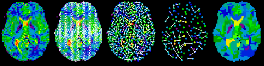
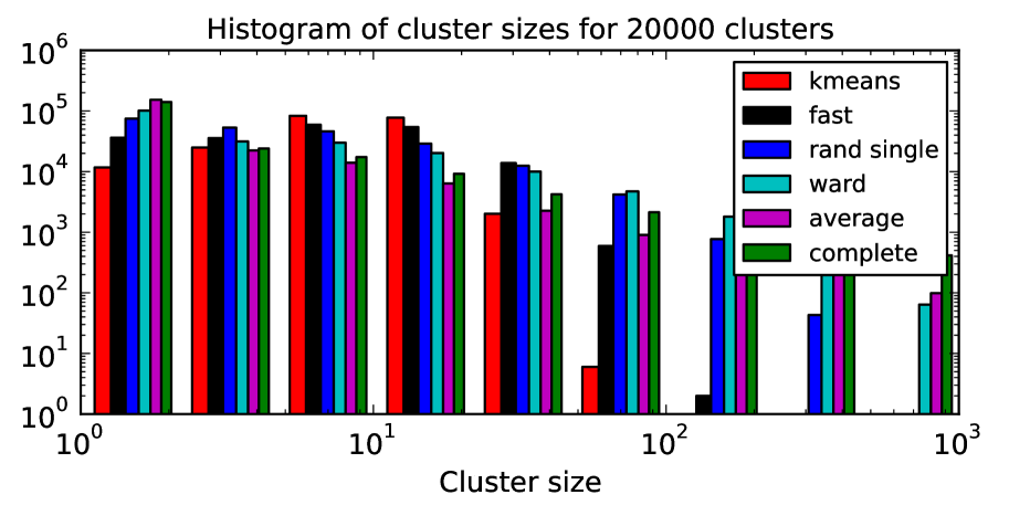
Figure 1: Principle of the fast clustering procedure illustrated in a real 2D brain image: the (non-percolating) nearest neighbor graph is computed from the origin data and so on recursively. At the last iteration, only the closest neighbors are associated to yield exactly the desired number $k$ of components.

Figure 2: Percolation behavior of various clustering methods observed through the cluster size histogram for a fixed number $k=20,000$ of clusters, obtained by averaging across 10 subjects of the HCP dataset. K-means and fast clustering best avoid percolation, as they display neither singletons nor very large clusters. Traditional agglomerative clustering methods, on the other hand, exhibit both giant and small components. Similar results are obtained for other values of $k$ and datasets.

4 Experiments

We compare the performance of various compression schemes: single, average and complete linkage, Ward, fast clustering and sparse random projections in a series of tasks involving public neuroimaging datasets (either anatomical or functional). We do not further study k-means, as the estimation is overly expensive in the large $k$ regime of interest.

Accuracy of the compressed representation

First, we study the accuracy of the isometry in Eq. 1, which we simply check empirically by evaluating the ratio $\eta=\frac{\|f(\mathbf{x}_{1})-f(\mathbf{x}_{2})\|^{2}}{\|\mathbf{x}_{1}-\mathbf{x}_{2}\|^{2}}$ for pairs ($\mathbf{x}_{1}$, $\mathbf{x}_{2}$) of samples on simulated and real data. Random projections come with precise guarantees on the variance of $\eta$ as a function of $k$, but no such result exists for cluster-based representations. The simulated data is simply a cube of shape $50\times 50\times 50$, that contains a signal consisting of smooth random signal (FWHM=8mm), with additional white noise; $n=100$ samples are drawn. The experimental data are a sample of 10 individuals taken from NYU test-retest resting-state functional Magnetic Resonance Imaging (fMRI) dataset (Shehzad et al., 2009), after preprocessing with a standard SPM8 pipeline, sampled at 3mm resolution in the MNI space ($n=197$ images per subject, $p=43878$ voxels).

To avoid the bias inherent to learning the clusters and measuring the accuracy of the representation on the same data, we perform a cross-validation loop: the clusters a learned on a training dataset, while the accuracy is measured on an independent dataset. Importantly, it can be observed that clustering is actually systematically compressive. Hence, we base our conclusions on the variance of $\eta$ across pairs of samples, i.e. the stability of the ratio between distances.

Noise reduction

To assess the differential effect of the spatial compressions on the signal and the noise, we considered a set of activation maps. Specifically, we relied on the motor activation dataset taken from 67 subjects of the HCP dataset (Barch et al., 2013), from which we considered the activation maps related to five different contrasts: (moving the) left hand versus average (activation), right hand vs. average, left foot vs. average, right foot vs. average and tongue vs average. These activation maps have been obtained by general linear model application upon the preprocessed data resampled at 2mm resolution in MNI space. From these sets of maps, in each voxel we computed the ratio of the between-condition variance (averaged across subjects) to the between-subject variance (averaged across conditions). Then we did the same on the fast cluster-based representation. The quotient of these two values is equal to 1 whenever the signals are identical. Values greater than 1 indicate a denoising effect, as the between-condition variance reflects the signal of interest while between-subject variance is expected to reflect noise plus between-subject variability. We simply consider the boxplot of the log of this ratio, as a function of the number $k$ of components.

Fast logistic regression

We performed a discriminative analysis on the OASIS dataset (Marcus et al., 2007): We used $n=403$ anatomical images and processed them with the SPM8 software to obtain modulated grey matter density maps sampled in the MNI space at 2mm resolution. We used these maps to predict the gender of the subject. To achieve this, the images were masked to an approximate average mask of the grey matter, leaving $p=140,398$ voxels. The voxel density values were then analyzed with an $\ell_{2}$-logistic classifier, the regularization parameter of which was set by cross-validation. This was performed for the following methods: non-reduced data, fast clustering, Ward and random projection reduction to either $k=4,000$ or $k=20,000$ components. The accuracy of the procedure was assessed in a 10-fold cross validation loop. We measured the computation time taken to reach a stable solution by varying the convergence control parameter.

Note that the estimation problem is rotationally invariant –i.e. the objective function is unchanged by a rotation of the feature space– which makes it well suited for projection-based dimension reductions. Indeed, these can be interpreted as a kernel.

Fast Independent Components Analysis

We performed an Independent Components Analysis (ICA) on resting state fMRI from the HCP dataset, as this is a task performed routinely on this dataset. Specifically, ICA is used to separate functional connectivity signal from noise and obtain a spatial model of the functional connectome (Smith et al., 2013). In the present experiment we analyzed independently data from 93 subjects. These data consist of two resting-state sessions of 1200 scans. We relied on the preprocessed data, resampled at 2mm resolution in the MNI space. Each image represents about 1GB of data, that is converted to a data matrix with ($p\approx 220,000$, $n=1,200$).

We performed an ICA analysis of each dataset in three settings: i) on the raw data, ii) on the data compressed by fast clustering ($k=20,000$) and iii) on the data compressed by sparse random projections ($k=20,000$). We extracted $q=40$ independent components as it is a standard number in the literature. Based on these analyses we investigated i) whether the components obtained from each dataset were similar or not before and after clustering; ii) How similar the components of session 1 and session 2 were after each type of processing. This was done by matching the components across sessions with the Hungarian algorithm, using the absolute value of the pairwise correlation as a between-components similarity; iii) the computation time of the ICA decomposition.

Implementation aspects

The data that we used are the publicly available NYU test-retest, OASIS and HCP datasets, for which we used the data with the preprocessing steps provided in the release 500-subjects release. We relied on the Scikit-learn library (Pedregosa et al., 2011) (v0.15) for machine learning tasks (ICA, logistic regression) and for Ward clustering. We relied on the Scipy library for the agglomerative clustering methods and the use of sparse matrices.

5 Results

Computational cost.

The computational cost of the different compression schemes is displayed in Fig. 5. While sparse random projections are obviously faster, as they do not require any training, fast clustering outperforms by far Ward clustering, which is much faster than average or complete linkage procedures. The clustering of a relatively large image can be obtained in a second, this cost is actually much smaller than standard linear algebra computations on the same dataset (blas level 3 operations). Furthermore, this cost is reduced by learning the clustering on a subset of the images (e.g. from 2.3s to 0.6s if one uses 10 images of OASIS instead of 100).

Accuracy of the compressed representation

The quality of distance preservation is summarized in Fig. 5. The random projections accuracy improves with $k$, as predicted by theory. Among the clustering algorithms, Ward clustering performs best in terms of distance preservation. Fast clustering performs slightly worse, though better than random projections. On the other hand, average and complete linkage perform poorly on this task –which is expected, due to their tendency toward percolation. In the next experiments, we only consider Ward and fast clustering.

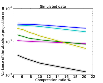
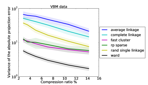
Figure 3: Evaluation of the computation time of the clustering algorithms (to obtain $k=10,000$ clusters) tested on $n=100$ images taken from the OASIS dataset. The proposed fast clustering outperforms by far all alternatives, except random projections.

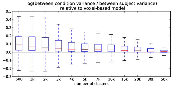
Figure 4: Evaluation of the metric accuracy of the compressed representations obtained through various compression techniques, for different numbers of components. These experiments are based on simulated (left) and the OASIS dataset (right) respectively. The compression ratio is $\frac{k}{p}$ and error bars are across 10 datasets;

Figure 5: Denoising effect of cluster-based compression: the ratio of between-contrasts (of interest) to between subject variance (of no interest) is increased when a lower number of regions is used in the data compression scheme. This is based on five motor contrasts of the HCP fMRI dataset and the fast clustering procedure.

Noise reduction

The differential effect of the spatial compression on the signal and the noise is displayed in Fig. 5. This shows that, in spite of large between-voxel variability, there is a clear trend toward a higher signal-to-noise ratio for lower values of k. This means that spatial compressions like clustering impose a low-pass filtering of the data that better preserves important discriminative features than variability components, part of which is simply noise.

Fast logistic regression.

The results of the application of logistic regression to the OASIS dataset are displayed in Fig. 7: this shows that the compressed datasets (with either fast clustering, Ward or random projections) can achieve at least the same level of accuracy as the uncompressed version, with drastic time savings. This result is a straightforward consequence of the approximate isometry property of the compressed representations. The accuracy achieved is actually higher for cluster-based compressions than with the original data or random projections: this illustrates again the denoising effect of spatial compression. As a side note, achieving full convergence did not improve the classifier performance. Qualitatively similar results are obtained with other rotationally invariant methods (e.g., $\ell_{2}$-SVMs, ridge regression). They should carry out to any kernel machine.

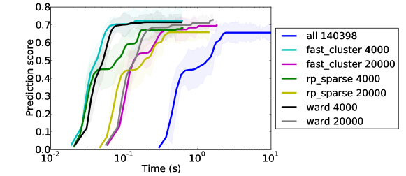
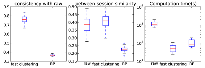
Figure 6: Quality of the fit of a logistic regression of the OASIS dataset as a function of computation time. The cluster-based methods obtain significantly higher scores than regression on the whole dataset with a much smaller computation time (by 1.5 orders of magnitude). Note that the time displayed does not include cluster computation, which is costly in the case of Ward clustering ($\approx$ 10 seconds, see Fig. 5).

Figure 7: Results of the ICA experiments (left) the accuracy of the fast clustering with respect to the non-compressed components is high. (Middle) across two sessions, fast clustering yields components more consistent than raw data, while random projections fail to do so; (right) Regarding computation time, fast clustering yields a gain factor of $\approx 20$, actually larger than $p/k$. The boxplots represent distributions across $93$ subjects.

Fast Independent Components Analysis

The results of the ICA experiment are summarized in Fig. 7: We found that the $q=40$ first components were highly similar before and after fast clustering: the average absolute correlation between the components was about $0.75$, while random projections do not recover the components (average correlation $<0.4$). Across two sessions, the components obtained by clustering are actually more similar after clustering than before, showing again the denoising effect of clustering. This effect was observed in all $93$ subjects, hence is extremely significant ($p<10^{-10}$, paired Wilcoxon rank test). On the opposite, random projections yielded a degradation of the similarity: this is because random projections perturb the statistical structure of the data, in particular the deviations from normality, which are used by ICA. As a consequence, ICA cannot recover the sources derived from the original data. By contrast, the statistical structure is mostly preserved after clustering. Finally, the computation time is reduced by a factor of 20, while $\frac{p}{k}\approx 12$ thus improving drastically the tractability of the procedure. Faster convergence is obtained by fast-clustering than with random projections. In summary, fast clustering not only helped to make ICA faster, it also improved the stability of the results. Random projections cannot be used for such a purpose.

6 Discussion

Our experiments have shown that on moderate size datasets, a fast clustering technique can yield impressive gains in computation speed for a minimal overhead to build the spatially- and contrast-aware data compression schemes. More importantly, the gain is found to be more than linear in various applications. This comes with two other good news: even in the absence of theoretical result, we found that spatial compression schemes perform as well as the state-of-the-art approach in data compression for machine learning, namely random projections. This holds thanks to the structure of medical images, where the noise is often observed in higher frequency components than the relevant information. Finally, we found that the spatial compression schemes presented here actually have a denoising effect, yielding possibly more accurate predictors than uncompressed version, or random projections.

Conceptually, it is tempting to compare the spatial model obtained with fast clustering with traditional brain parcellation or super-voxels. The difference lies in the interpretation: we do not view spatial compression as a meaningful model per se, but as a way to reduce data dimensionality without losing too much information. We will typically set $k=p/10$ and this number is necessarily a trade-off between computational efficiency and data fidelity. Note that in this regime, Ward clustering is slightly more powerful in terms of representation accuracy, but it is much slower hence cannot be considered as a practical solution.

As shown by the ICA experiment, clustering-based compression can be used even in tasks in which the $\ell_{2}$ norm preservation alone does not guarantee a good representation. The combination of clustering, randomization and sparsity has also proved to be an extremely effective tool in ill-posed multivariate estimation problems (Varoquaux et al., 2012; Bühlmann et al., 2012), hence fast clustering seems particularly well-suited for these problems.

In conclusion, we have shown that a procedure using our fast clustering method as a data reduction yields a speed up of 1.5 order of magnitude on two real-world multivariate statistic problems. Moreover, on a supervised problem, we improve the prediction performance by using our data compression scheme, as it captures better signal than noise. The proposed strategy is thus extremely promising regarding the statistical analysis of big medical image datasets, as it is perfectly compatible with efficient online estimation methods (Schmidt et al., 2013).

Acknowledgment.

Data were provided in part by the Human Connectome Project, WU-Minn Consortium (Principal Investigators: David Van Essen and Kamil Ugurbil; 1U54MH091657) funded by the 16 NIH Institutes and Centers that support the NIH Blueprint for Neuroscience Research; and by the McDonnell Center for Systems Neuroscience at Washington University.

References

- Baraniuk & Wakin (2009) Baraniuk, Richard G. and Wakin, Michael B. Random projections of smooth manifolds. Found. Comput. Math., 9(1):51–77, January 2009. ISSN 1615-3375.
- Barch et al. (2013) Barch, Deanna M, Burgess, Gregory C, Harms, Michael P, Petersen, Steven E, Schlaggar, Bradley L, Corbetta, Maurizio, Glasser, Matthew F, Curtiss, Sandra, Dixit, Sachin, Feldt, Cindy, Nolan, Dan, Bryant, Edward, Hartley, Tucker, Footer, Owen, Bjork, James M, Poldrack, Russ, Smith, Steve, Johansen-Berg, Heidi, Snyder, Abraham Z, Essen, David C Van, and Consortium, W. U-Minn HCP. Function in the human connectome: task-fmri and individual differences in behavior. Neuroimage, 80:169–189, Oct 2013.
- Bühlmann et al. (2012) Bühlmann, P., Rütimann, P., van de Geer, S., and Zhang, C.-H. Correlated variables in regression: clustering and sparse estimation. ArXiv e-prints, September 2012.
- Button et al. (2013) Button, Katherine S, Ioannidis, John P A, Mokrysz, Claire, Nosek, Brian A, Flint, Jonathan, Robinson, Emma S J, and Munafò, Marcus R. Power failure: why small sample size undermines the reliability of neuroscience. Nat Rev Neurosci, 14(5):365–376, May 2013.
- Felzenszwalb & Huttenlocher (2004) Felzenszwalb, Pedro F. and Huttenlocher, Daniel P. Efficient graph-based image segmentation. Int. J. Comput. Vision, 59(2):167–181, September 2004. ISSN 0920-5691.
- Halko et al. (2009) Halko, N., Martinsson, P.-G., and Tropp, J. A. Finding structure with randomness: Probabilistic algorithms for constructing approximate matrix decompositions. ArXiv e-prints, September 2009.
- Heinrich et al. (2013) Heinrich, Mattias P., Jenkinson, Mark, Papiez, Bartlomiej W., Glesson, Fergus V., Brady, Michael, and Schnabel, Julia A. Edge- and detail-preserving sparse image representations for deformable registration of chest mri and ct volumes. In IPMI, pp. 463–474, 2013.
- Johnson & Lindenstrauss (1984) Johnson, William and Lindenstrauss, Joram. Extensions of Lipschitz mappings into a Hilbert space. In Conference in modern analysis and probability, volume 26 of Contemporary Mathematics, pp. 189–206. American Mathematical Society, 1984.
- Li et al. (2006) Li, Ping, Hastie, Trevor J., and Church, Kenneth W. Very sparse random projections. In International Conference on Knowledge Discovery and Data Mining, KDD, pp. 287, 2006. ISBN 1-59593-339-5.
- Marcus et al. (2007) Marcus, Daniel S, Wang, Tracy H, Parker, Jamie, Csernansky, John G, Morris, John C, and Buckner, Randy L. Open access series of imaging studies (oasis): cross-sectional mri data in young, middle aged, nondemented, and demented older adults. J Cogn Neurosci, 19(9):1498–1507, Sep 2007.
- Pedregosa et al. (2011) Pedregosa, F., Varoquaux, G., Gramfort, A., Michel, V., Thirion, B., Grisel, O., Blondel, M., Prettenhofer, P., Weiss, R., Dubourg, V., Vanderplas, J., Passos, A., Cournapeau, D., Brucher, M., Perrot, M., and Duchesnay, E. Scikit-learn: Machine learning in Python. Journal of Machine Learning Research, 12:2825, 2011.
- Rahimi & Recht (2007) Rahimi, Ali and Recht, Ben. Random features for large-scale kernel machines. In In Neural Infomration Processing Systems, 2007.
- Schmidt et al. (2013) Schmidt, M., Le Roux, N., and Bach, F. Minimizing Finite Sums with the Stochastic Average Gradient. ArXiv e-prints, September 2013.
- Shehzad et al. (2009) Shehzad, Z., Kelly, AM, Reiss, P.T., Gee, D.G., Gotimer, K., Uddin, L.Q., Lee, S.H., Margulies, D.S., Roy, A.K., Biswal, B.B., et al. The resting brain: unconstrained yet reliable. Cerebral Cortex, 2009.
- Smith et al. (2013) Smith, Stephen M, Beckmann, Christian F, Andersson, Jesper, Auerbach, Edward J, Bijsterbosch, Janine, Douaud, Gwenaëlle, Duff, Eugene, Feinberg, David A, Griffanti, Ludovica, Harms, Michael P, Kelly, Michael, Laumann, Timothy, Miller, Karla L, Moeller, Steen, Petersen, Steve, Power, Jonathan, Salimi-Khorshidi, Gholamreza, Snyder, Abraham Z, Vu, An T, Woolrich, Mark W, Xu, Junqian, Yacoub, Essa, Uğurbil, Kamil, Essen, David C Van, Glasser, Matthew F, and Consortium, W. U-Minn HCP. Resting-state fmri in the human connectome project. Neuroimage, 80:144–168, Oct 2013.
- Stauffer & Aharony (1971) Stauffer, D. and Aharony, A. Introduction to Percolation Theory. Oxford University Press, New York, 1971.
- Teng & Yao (2007) Teng, Shang-Hua and Yao, FrancesF. k-nearest-neighbor clustering and percolation theory. Algorithmica, 49(3):192–211, 2007. ISSN 0178-4617. doi: 10.1007/s00453-007-9040-7. URL http://dx.doi.org/10.1007/s00453-007-9040-7.
- Varoquaux et al. (2012) Varoquaux, Gaël, Gramfort, Alexandre, and Thirion, Bertrand. Small-sample brain mapping: sparse recovery on spatially correlated designs with randomization and clustering. In ICML, pp. 1375, 2012.
- Ward (1963) Ward, Joe H. Hierarchical grouping to optimize an objective function. Journal of the American Statistical Association, 58:236, 1963.
- Zalesky et al. (2014) Zalesky, Andrew, Fornito, Alex, Cocchi, Luca, Gollo, Leonardo L, and Breakspear, Michael. Time-resolved resting-state brain networks. Proc Natl Acad Sci U S A, 111:10341–10346, 2014.