UCHEP–15–03

CHARM 2015 Experimental Summary: Step-by-Step Towards New Physics

A. J. Schwartz

Physics Department
University of Cincinnati, Cincinnati, Ohio 44221 USA

The experimental program of the Seventh International Workshop on Charm Physics (CHARM 2015) is summarized. Highlights of the workshop include results from heavy flavor production, quarkonium and exotic states, hadronic decays and Dalitz analyses, semileptonic and leptonic decays, rare and radiative decays, charm mixing, and $CP$ and $T$ violation.

PRESENTED AT

The 7th International Workshop on Charm Physics (CHARM 2015)
Detroit, MI, 18-22 May, 2015

1 Introduction

This year’s workshop featured almost fifty experimental talks covering a wide variety of charm physics results. The presentations can be categorized as follows: heavy flavor production; quarkonium and exotic states; hadronic decays and Dalitz analyses; semileptonic decays; leptonic decays; rare and radiative decays; $CP$ violation and mixing; beyond-the-Standard-Model searches; charm baryons, $\tau$ leptons, and other miscellaneous decays. Results were presented from Belle, BaBar, CLEOc, BESIII, CDF, D0, ATLAS, CMS, LHCb, STAR, PHENIX, and ALICE experiments. In this review I discuss some of the highlights from among these talks. Space constraints allow for only a cursory discussion, and for more details the reader is referred to the original presentation and writeup.

2 Production

Numerous results were presented on $D$ meson production in proton-nucleus and nucleus-nucleus collisions (Dainese). The temperatures of such collisions correspond to the environment of a quark-gluon plasma (QGP), and partons produced in the collision interact with the QGP when escaping, resulting in an energy loss. The parton energy loss is expected to decrease as the parton mass increases. The parameter quantifying parton interaction with the QGP is the “nuclear modification factor:”

$$R_{AA}(p_{T}\/) \equiv \frac{1}{N_{\rm coll}}\frac{(dN_{AA}/dp_{T})}{(dN_{pp}/dp_{T})}\,,$$ (1)

where $N~{}{}_{\rm coll}$ is the number of nucleons participating in the collision. The greater the interaction with the QGP and subsequent energy loss, the lower $R_{AA}(p_{T}\/)$; this is referred to as “suppression.” The amount of suppression is found to increase with $p_{T}$; typical behavior is shown in Fig. 1(left), which plots Pb-Pb data taken by the ALICE experiment. Suppression also depends upon the nuclei colliding: using $\pi^{0}$ production and also electrons from heavy flavor decays, PHENIX shows that in Au-Au collisions suppression is significant, but in $d$-Au collisions it is not. ALICE confirms this trend for $D^{0}$ production by reconstructing $D^{0}\!\rightarrow\!K^{-}\pi^{+}$ decays [1]: in Pb-Pb collisions $D^{0}$ suppression is significant, while in $p$-Pb collisions it is not.

Finally, suppression also depends on the “centrality” of a collision, i.e., the amount of overlap of the colliding hadronic systems. The centrality of a collision is inferred from the multiplicity of secondary particles produced: a high multiplicity of secondaries indicates large hadronic overlap. Data from ATLAS shows that suppression is largest for central collisions and smallest for peripheral collisions, for several ranges of $p_{T}\/$ studied.

CMS reconstructs $J/\psi$ decays in Pb-Pb collisions and, by requiring that the $J/\psi$ have large impact parameter, identifies these $J/\psi$’s as originating from $B$ decays [2]. Comparing $R_{AA}$ for this $B$ sample with $R_{AA}$ measured by ALICE for $D$ decays shows that $R^{B}_{AA}>R^{D}_{AA}$ [Fig. 1(right)], as expected because $m_{b}>m_{c}$. This is an important confirmation of this relationship.

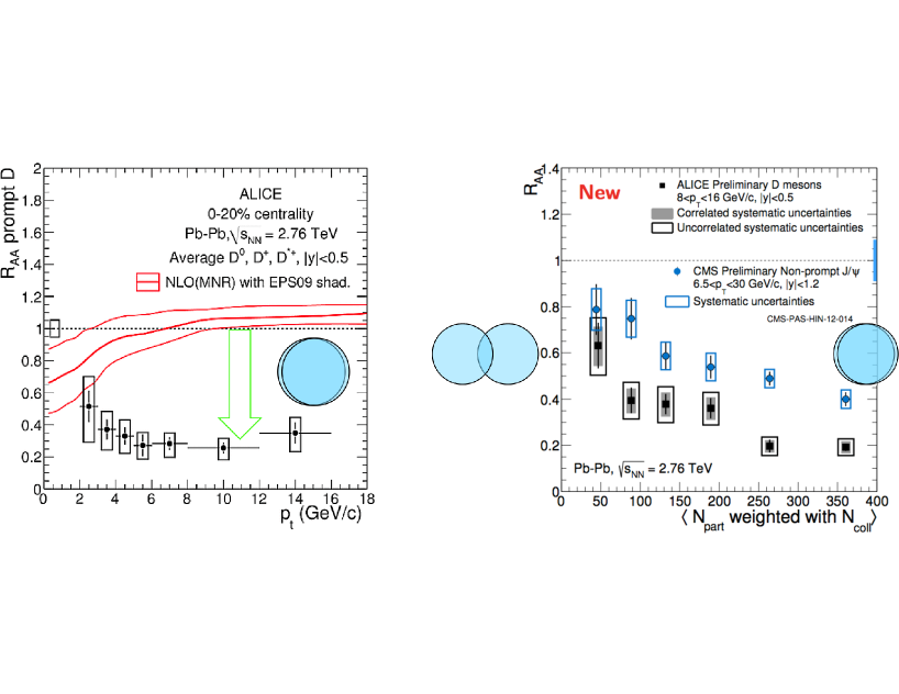
Figure 1: Left: $R^{D}_{AA}$ measured by ALICE in Pb-Pb collisions using $D^{0}\!\rightarrow\!K^{-}\pi^{+}$ decays. Right: $R_{AA}$ plotted vs. $N_{\rm part}$, where higher (lower) values correspond to central (peripheral) collisions. Included in this plot is $R^{B}_{AA}$ measured by CMS in Pb-Pb collisions using non-prompt $J/\psi$ decays [2]. The data shows that $R^{B}_{AA}>R^{D}_{AA}$, as expected.

3 X/Y/Z Quarkonia

Results for $X/Y/Z$ states were presented by BESIII, Belle, and ATLAS. A subset of these results are summarized below.

3.1 BESIII

BESIII (Kornicer, Lyu, Prasad) selects $e^{+}e^{-}\!\rightarrow\!(J/\psi,h_{c})\pi^{+}\pi^{-}$ and $(J/\psi,h_{c})\pi^{0}\pi^{0}$ decays, where $J/\psi\!\rightarrow\!\ell^{+}\ell^{-}$ and $h_{c}(1P)\!\rightarrow\!\eta_{c}\gamma$, and plots the invariant mass of the $J/\psi\,\pi$ and $h_{c}\pi$ combinations. In the $J/\psi$ sample, prominent peaks are observed for $Z_{c}(3900)^{+}$ and $Z_{c}(3900)^{0}$ states; in the $h_{c}$ sample, peaks are observed for $Z_{c}(4020)^{+}$ and $Z_{c}(4020)^{0}$ states. The fitted masses with systematic errors are listed in Table 1.

State	Fitted mass
$M_{Z_{c}(3900)^{+}}$	$3899.0\pm 3.6\pm 4.9$
$M_{Z_{c}(3900)^{0}}$	$3894.8\pm 2.3\pm 2.7$
$M_{Z_{c}(4020)^{+}}$	$4022.9\pm 0.8\pm 2.7$
$M_{Z_{c}(4020)^{0}}$	$4023.9\pm 2.2\pm 3.8$

Table 1: States observed by BESIII in $e^{+}e^{-}\!\rightarrow\!(J/\psi,h_{c})\pi^{+}\pi^{-}$ and $(J/\psi,h_{c})\pi^{0}\pi^{0}$ reactions, and the fitted masses with systematic errors.

BESIII also selects $e^{+}e^{-}\!\rightarrow\!\pi^{-}(D\overline{D}^{*})^{+}$ events. Plotting the invariant mass of the $(D\overline{D}^{*})^{+}$ pair shows an enhancement just above threshold, which may be an isospin partner of the $X(3872)$; the fitted mass is $3884.3\pm 1.2\pm 1.5$. Selecting $e^{+}e^{-}\!\rightarrow\!J/\psi\,\pi^{+}\pi^{-}\gamma$ events and plotting the $J/\psi\,\pi^{+}\pi^{-}$ three-body mass shows a sharp peak at the $X(3872)$; the fitted mass is $3871.9\pm 0.7\pm 0.2$. BESIII measures the cross section for this reaction at three different center-of-mass energies and observes a rise in the cross section that is consistent with a Breit-Wigner lineshape from the $Y(4260)$; this is suggestive of $Y(4260)\!\rightarrow\!X(3872)\gamma$ decays. The measured rate would correspond to a ratio ${\cal B}(Y_{4260}\!\rightarrow\!X_{3872}\gamma)/{\cal B}(Y_{4260}\!\rightarrow\!J/\psi\,\pi^{+}\pi^{-})\approx 0.10$, which, if true, implies that the $X(3872)$ and $Y(4260)$ are related.

Finally, BESIII reconstructs $e^{+}e^{-}\!\rightarrow\!\chi_{c}\pi^{+}\pi^{-}\gamma$ events, where $\chi_{c}\!\rightarrow\!J/\psi\,\gamma$. Plotting the $\pi^{+}\pi^{-}$ recoil mass exhibits a new $X(3823)$ state [Fig. 2(left)]. The significance is $6.7\sigma$, and the fitted mass and width are $M=3821.7\pm 1.3\pm 0.7$ and $\Gamma<16$ MeV at 90% C.L. These values are consistent with those expected for the $\psi(1^{3}D_{2})$ state, and BESIII may be observing $e^{+}e^{-}\!\rightarrow\!\psi(1^{3}D_{2})\pi^{+}\pi^{-},\,\psi(1^{3}D_{2})\!\rightarrow\!\chi_{c}\gamma$ reactions.

3.2 Belle

Belle (Wang, Bhardwaj) showed results for $X/Y/Z$ states produced in $B$ decays. The decays $B^{\pm}\!\rightarrow\!K^{\pm}\eta_{c}h$ are reconstructed, where $h=\omega,\,\eta,\,\pi^{0},\,\pi^{+}\pi^{-}$, and the $\eta_{c}h$ mass spectrum is studied for evidence of $X(3730),\,X(3872),\,X(3915),\,X(4014),\,Z(3900)$ and $Z(4020)$ states. No evidence is seen for any of these states, and upper limits are set for the branching fractions $B^{\pm}\!\rightarrow\!K^{\pm}(X,Z),\,(X,Z)\!\rightarrow\!\eta_{c}h$. These limits lie in the range $(1.2-6.9)\times 10^{-5}$.

Belle also presented results for $Y(4360)$ and $Y(4660)$ production and decay. First, $B^{+}\!\rightarrow\!\psi(2S)\pi^{+}\pi^{-}K^{+}$ decays are reconstructed and the $\psi(2S)\pi^{+}\pi^{-}$ mass distribution is plotted, where $\psi(2S)\!\rightarrow\!J/\psi\,\pi^{+}\pi^{-}$ or $\mu^{+}\mu^{-}$. Both mass distributions show prominent peaks for the $Y(4360)$ and $Y(4660)$ states; the combined distribution is shown in Fig. 2(right). Fitting the peaks to Breit-Wigner amplitudes yields the parameters listed in Table 2. In a second analysis the $Y(4360)$ is produced directly via $e^{+}e^{-}\!\rightarrow\!\psi(2S)\pi^{+}\pi^{-}$ [3]. The final state is reconstructed as a function of center-of-mass energy ($\sqrt{s}$), and peaks are seen at $\sqrt{s}\approx 4350$ MeV and 4650 MeV. The $Y(4360)$ peak corresponds to a cross section of $\sim$ 75 pb, which is surprisingly close to the cross sections measured previously by Belle for $e^{+}e^{-}\!\rightarrow\!Y(4260)\!\rightarrow\!J/\psi\,\pi^{+}\pi^{-}$ and $e^{+}e^{-}\!\rightarrow\!\psi(4040)\!\rightarrow\!J/\psi\,\eta$ reactions [4, 5].

State	Fitted mass ( MeV/$c^{2}$)	Fitted width ( MeV)
$Y(4360)$	$4347\,\pm 6\,\pm 3$	$103\,\pm 9\,\pm 5$
$Y(4660)$	$4652\,\pm 10\,\pm 11$	$68\,\pm 11\,\pm 5$

Table 2: Parameters measured by Belle by fitting the $\psi(2S)\pi^{+}\pi^{-}$ invariant mass spectrum in $B^{\pm}\!\rightarrow\!\psi(2S)\pi^{+}\pi^{-}K^{\pm}$ decays.

Finally, Belle searched for $X(3872)$ production via $B^{0}\!\rightarrow\!X(3872)K^{+}\pi^{-}$ and $B^{+}\!\rightarrow\!X(3872)K^{0}_{S}\,\pi^{+}$, where $X(3872)\!\rightarrow\!J/\psi\,\pi^{+}\pi^{-}$. In both cases clear peaks are observed above background; the signal significances are $7.0\sigma$ and $3.7\sigma$, respectively. The number of signal candidates for the more copious neutral mode is $151\pm 21$, and the product of branching fractions is ${\cal B}(B^{0}\!\rightarrow\!X(3872)K^{+}\pi^{-})\times{\cal B}(X(3872)\!\rightarrow\!J/\psi\,\pi^{+}\pi^{-})=(7.9\,\pm 1.3\,\pm 0.4)\times 10^{-6}$. The $K^{+}\pi^{-}$ mass spectrum is subsequently fitted to identify $K^{*}(890)$ production, and the resonant fraction is measured to be

$$\frac{{\cal B}(B^{0}\!\rightarrow\!X(3872)K^{*0})\times{\cal B}(K^{*0}\!\rightarrow\!K^{+}\pi^{-})}{{\cal}{\cal B}(B^{0}\!\rightarrow\!X(3872)K^{+}\pi^{-})} = 0.34\,\pm 0.09\,\pm 0.02\,.$$ (2)

       

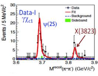
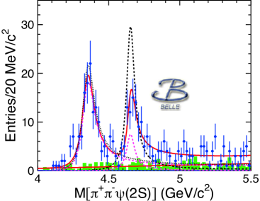
Figure 2: Left: BESIII measurement of the $\pi^{+}\pi^{-}$ recoil mass in $e^{+}e^{-}\!\rightarrow\!\pi^{+}\pi^{-}\chi_{c}\gamma$ reactions. The rightmost peak indicates $X(3823)\!\rightarrow\!\chi_{c}\gamma$ decays. Right: Belle measurement of the $\psi(2S)\pi^{+}\pi^{-}$ mass spectrum in $B^{+}\!\rightarrow\!\psi(2S)\pi^{+}\pi^{-}K^{+}$ decays, where $\psi(2S)\!\rightarrow\!(J/\psi\,\pi^{+}\pi^{-},\,\mu^{+}\mu^{-})$. The peaks indicate $Y(4360)\!\rightarrow\!\psi(2S)\pi^{+}\pi^{-}$ and $Y(4660)\!\rightarrow\!\psi(2S)\pi^{+}\pi^{-}$ decays. The results of fitting to Breit-Wigner amplitudes are superimposed.

4 Hadronic Decays

Results for hadronic decays, including several Dalitz analyses, were presented by BESIII, BaBar, and LHCb, as summarized below.

4.1 BESIII

BESIII (Wiedenkaff, Muramatsu) reported measurements of singly Cabibbo-suppressed decays of $D$ mesons: $D^{+}\!\rightarrow\!\omega\pi^{+}$, $D^{0}\!\rightarrow\!\omega\pi^{0}$, $D^{+}\!\rightarrow\!\eta\pi^{+}$, and $D^{0}\!\rightarrow\!\eta\pi^{0}$. The results are listed in Table 3. For the final states with $\omega$, these results provide the first evidence for these decays.

Mode	Branching fraction	PDG value
$D^{+}\!\rightarrow\!\omega\pi^{+}$	$(2.74\,\pm 0.58\,\pm 0.17)\times 10^{-4}$	$<3.4\times 10^{-4}$ (90% C.L.)
$D^{0}\!\rightarrow\!\omega\pi^{0}$	$(1.05\,\pm 0.41\,\,\pm 0.09)\times 10^{-4}$	$<2.6\times 10^{-4}$ (90% C.L.)
$D^{+}\!\rightarrow\!\eta\pi^{+}$	$(3.13\,\pm 0.22\,\pm 0.19)\times 10^{-3}$	$(3.53\,\pm 0.21)\times 10^{-3}$
$D^{0}\!\rightarrow\!\eta\pi^{0}$	$(0.67\,\pm 0.10\,\pm 0.05)\times 10^{-3}$	$(0.68\,\pm 0.07)\times 10^{-3}$

Table 3: BESIII measurements of singly Cabibbo-suppressed decays.

4.2 BaBar

BaBar (Palano) reported results of a model-independent Dalitz analysis of four decay modes: $\eta_{c}\!\rightarrow\!K^{+}K^{0}_{S}\,\pi^{-}$, $\eta_{c}\!\rightarrow\!K^{+}K^{-}\pi^{0}$, $J/\psi\!\rightarrow\!\pi^{+}\pi^{-}\pi^{0}$, and $J/\psi\!\rightarrow\!K^{+}K^{-}\pi^{0}$. For all modes an unbinned likelihood fit is performed for magnitudes and phases in 30 bins of $K\pi$ or $\pi\pi$ invariant mass. Both $\eta_{c}\!\rightarrow\!K^{+}K\pi$ samples show clear evidence for the $K^{*0}(1430)$ resonance: at this mass value the magnitude reaches a maximum and the phase passes through 90^∘ (see Fig. 3). This behavior differs somewhat from that observed in a model-independent Dalitz analysis of $D^{+}\!\rightarrow\!K^{+}\pi^{+}\pi^{-}$ decays by FNAL E791 [6].

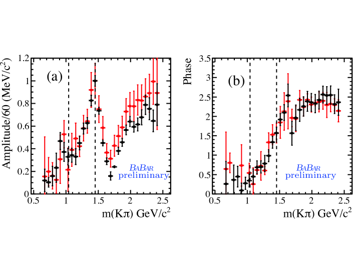
Figure 3: BaBar results for (a) magnitudes and (b) phases in bins of $M_{K\pi}$ from a Dalitz analysis of $\eta_{c}\!\rightarrow\!K^{+}K^{0}_{S}\,\pi^{-}$ (black) and $\eta_{c}\!\rightarrow\!K^{+}K^{-}\pi^{0}$ (red) decays. The dashed lines indicate the $K\eta$ and $K\eta^{\prime}$ thresholds. The distributions indicate the presence of the $K^{*}(1430)$ resonance.

BaBar also reported a search for anomalous structure (Sokoloff). A sample of $B$ decays was fully reconstructed, and, among the remaining tracks, a $K^{+}$ was required and its momentum plotted. A sharp peak in this spectrum would indicate a two-body decay $B\!\rightarrow\!K^{+}X$ of the other $B$ in the event. Both $B^{0}$ and $B^{+}$ samples were analyzed, and several momentum peaks were observed corresponding to decays $B\!\rightarrow\!DK^{+}$, $B\!\rightarrow\!D^{*}K^{+}$, and $D^{**}(2420)K^{+}$. A sharp peak was observed in the $B^{+}$ sample corresponding to $B^{+}\!\rightarrow\!\overline{D}^{\,**0}(2680)K^{+}$, but no analogous peak was seen in the $B^{0}$ sample.

4.3 LHCb

LHCb (Palano again) presented Dalitz analyses for the modes $B^{-}\!\rightarrow\!D^{+}K^{-}\pi^{-}$, $B^{0}\!\rightarrow\!\overline{D}{}^{\,0}\pi^{+}\pi^{-}$, $B^{0}\!\rightarrow\!\overline{D}{}^{\,0}K^{+}\pi^{-}$, and $B^{0}_{s}\!\rightarrow\!\overline{D}{}^{\,0}K^{-}\pi^{+}$. These analyses fit the data using isobar models. For $B^{-}\!\rightarrow\!D^{+}K^{-}\pi^{-}$, the well-known resonances $D^{*}_{0}(2400)^{0}$, $D^{*}_{2}(2460)^{0}$, and $D^{*}_{1}(2760)^{0}$ are observed. The resulting fit fractions are listed in Table 4.

Resonance	Fit fraction
$D^{*}_{0}(2400)^{0}$	$\phantom{2}8.3\pm 2.6\pm 0.6\pm\phantom{2}1.9$
$D^{*}_{2}(2460)^{0}$	$31.8\pm 1.5\pm 0.9\pm\phantom{2}1.4$
$D^{*}_{1}(2760)^{0}$	$\phantom{2}4.9\pm 1.2\pm 0.3\pm\phantom{2}0.9$
$S$-wave non-resonant	$38.0\pm 7.4\pm 1.5\pm 10.8$
$P$-wave non-resonant	$23.8\pm 5.6\pm 2.1\pm\phantom{2}3.7$
$D^{*}_{v}(2007)^{0}$	$\phantom{2}7.6\pm 2.3\pm 1.3\pm\phantom{2}1.5$
$B^{*}_{v}$	$\phantom{2}3.6\pm 1.9\pm 0.9\pm\phantom{2}1.6$

Table 4: LHCb results for fitted fractions (%) in $B^{-}\!\rightarrow\!D^{+}K^{-}\pi^{-}$ decays. The errors listed are statistical, experimental systematic, and model uncertainties, respectively [7].

LHCb also reported a measurement of $B^{+}\!\rightarrow\!X(3872)K^{+},\,X(3872)\!\rightarrow\!J/\psi\,\rho^{0}$ decays. The experiment reconstructs 1011 candidates with a purity of 80%. By fitting the helicity angle distribution, LHCb confirms that the $X(3872)$ has quantum numbers $J^{PC}=1^{++}$.

5 Semileptonic Decays

5.1 BESIII

BESIII (An, Ma) presented results for several semileptonic decays. For $D^{+}\!\rightarrow\!K^{-}\pi^{+}e^{+}\nu$ they measure the branching fraction to be $(3.71\,\pm 0.03\,\pm 0.09)$%. Most of the $K^{-}\pi^{+}$ pairs originate from $K^{*0}$ decays; requiring $M_{K\pi}\in(0.8,1.0)$ GeV/$c^{2}$ yields a branching fraction of $(3.33\,\pm 0.03\,\pm 0.08)$%. For $D^{+}\!\rightarrow\!\omega e^{+}\nu$ BESIII observes a significant signal and measures a branching fraction of $(1.63\,\pm 0.11\,\pm 0.08)\times 10^{-3}$. The statistics are sufficient to extract form factor parameters for the first time; the results are $r_{V}\equiv V(0)/A_{1}(0)=1.24\,\pm 0.09\,\pm 0.06$ and $r_{2}\equiv A_{2}(0)/A_{1}(0)=1.06\,\pm 0.15\,\pm 0.05$. Finally, results for $D^{+}\!\rightarrow\!K_{L}e^{+}\nu$ were presented. The branching fraction is measured to be $(4.482\,\pm 0.027\,\pm 0.103)$%, and the form factor parameters are $|V_{cs}|f^{K}_{+}(0)=0.728\,\pm 0.006\,\pm 0.011$ and $r_{1}\equiv a_{1}/a_{0}=1.91\,\pm 0.33\,\pm 0.24$. As this final state is self-tagging, signal events are subsequently divided into $e^{+}$ and $e^{-}$ subsamples and the $CP$ asymmetry measured. The result is $A^{K_{L}e\nu}_{CP}=(-0.59\,\pm 0.60\,\pm 1.50)$%.

5.2 BaBar

BaBar (Oyanguren) measures the branching fraction for $D^{0}\!\rightarrow\!\pi^{-}e^{+}\nu$ decays normalized to $D^{0}\!\rightarrow\!K^{-}\pi^{+}$ decays. To reduce backgrounds they require that the $D^{0}$ originate from $D^{*+}\!\rightarrow\!D^{0}\pi^{+}_{s}$ decays. The signal yield is obtained by fitting the $\Delta M=M_{(\pi e\nu)\pi^{+}_{s}}-M_{\pi e\nu}$ distribution. The resulting ratio of branching fractions is

$$R_{D} \equiv \frac{{\cal B}(D^{0}\!\rightarrow\!\pi^{-}e^{+}\nu)}{{\cal B}(D^{0}\!\rightarrow\!K^{-}\pi^{+})}\ =\ 0.0702\,\pm 0.0017\,\pm 0.0023\,.$$ (3)

Using the world average value for ${\cal B}(D^{0}\!\rightarrow\!K^{-}\pi^{+})$ yields ${\cal B}(D^{0}\!\rightarrow\!\pi^{-}e^{+}\nu)=(2.770\,\pm 0.068\,\pm 0.092\,\pm 0.037)\times 10^{-3}$, where the last error is from ${\cal B}(D^{0}\!\rightarrow\!K^{-}\pi^{+})$. BaBar subsequently fits the $z$(-expansion) distribution to measure the normalization factor $|V_{cd}|f^{\pi}_{+}(0)=0.1374\,\pm 0.0038\,\pm 0.0022\,\pm 0.0009_{\rm ext}$, where the last error is due to external factors not directly related to the experimental measurement. Inserting $|V_{cd}|=|V_{us}|=0.2252\,\pm 0.0009$ [8] gives a form factor normalization $f^{\pi}_{+}(0)=0.610\,\pm 0.017\,\pm 0.010\,\pm 0.005_{\rm ext}$. Alternatively, inserting the average form factor from lattice QCD (LQCD) calculations, $f^{\pi}_{+}(0)=0.666\,\pm 0.029$ [9], gives $|V_{cd}|=0.206\,\pm 0.007_{\rm exp}\,\pm 0.009_{\rm LQCD}$. This value is consistent within errors with the current world average as calculated by HFAG using $D\!\rightarrow\!\pi\ell\nu$ and $D\!\rightarrow\!\ell\nu$ decays: $0.219\pm 0.006$ [10].

6 Leptonic Decays

BESIII (Ma) presented results for purely leptonic $D^{+}\!\rightarrow\!e^{+}\nu,\,\mu^{+}\nu,\,\tau^{+}\nu$ decays, and Belle (Eidelman) presented results for leptonic $D^{+}_{s}\!\rightarrow\!e^{+}\nu,\,\mu^{+}\nu,\,\tau^{+}\nu$ decays. The branching fractions are used to determine the products of decay constants multiplied by CKM matrix elements $f_{D}|V_{cd}|$ and $f_{D_{s}}|V_{cs}|$, respectively. The Belle results are the world’s most precise.

It is notable that the current world average for $|V_{cd}|$ [10] is dominated by measurements of purely leptonic $D^{+}\!\rightarrow\!e^{+}\nu,\,\mu^{+}\nu,\,\tau^{+}\nu$ decays: $0.219\,\pm 0.005\,\pm 0.003$. This value has a smaller overall error than that obtained from semileptonic $D^{0}\!\rightarrow\!\pi^{-}\ell^{+}\nu$ decays, $0.214\,\pm 0.003\,\pm 0.009$. Similarly, the current world average for $|V_{cs}|$ [11] ($0.998\,\pm 0.020$) is dominated by measurements of leptonic $D^{+}_{s}\!\rightarrow\!e^{+}\nu,\,\mu^{+}\nu,\,\tau^{+}\nu$ decays, $1.008\,\pm 0.018\,\pm 0.011$, i.e., the overall error is (slightly) smaller than that obtained from semileptonic $D^{0}\!\rightarrow\!K^{-}\ell^{+}\nu$ decays, $0.975\,\pm 0.007\,\pm 0.025$.

7 Rare, Forbidden, and Radiative Decays

7.1 BESIII

BESIII (Zhao) presented results for flavor-changing neutral-current (FCNC) and lepton-number-violating (LNV) decays of $D^{+}_{(s)}$ mesons involving electrons; these are summarized in Table 5. In all cases no signal was observed and upper limits were set. For $D^{+}\!\rightarrow\!K^{-}e^{+}e^{+}$ and $D^{+}_{s}\!\rightarrow\!\pi^{+}e^{+}e^{-}$, these limits are the world’s most stringent. BESIII also obtained an upper limit for the purely radiative decay $D^{0}\!\rightarrow\!\gamma\gamma$ (Table 5); however, this limit is almost twice the corresponding upper limit set by BaBar [12].

Mode	90% C.L. upper limit	PDG upper limit
$D^{+}\!\rightarrow\!K^{+}e^{+}e^{-}$	$1.2\times 10^{-6}$	$1.0\times 10^{-6}$
$D^{+}\!\rightarrow\!K^{-}e^{+}e^{+}$	$0.6\times 10^{-6}$	$0.9\times 10^{-6}$
$D^{+}_{s}\!\rightarrow\!\pi^{+}e^{+}e^{-}$	$0.3\times 10^{-6}$	$1.1\times 10^{-6}$
$D^{+}_{s}\!\rightarrow\!\pi^{-}e^{+}e^{+}$	$1.2\times 10^{-6}$	$1.1\times 10^{-6}$
$D^{0}\!\rightarrow\!\gamma\gamma$	$3.8\times 10^{-6}$	$2.2\times 10^{-6}$

Table 5: 90% C.L. upper limits from BESIII for FCNC and LNV decays, and for the radiative decay $D^{0}\!\rightarrow\!\gamma\gamma$ [13].

7.2 LHCb

LHCb (Göbel, Vacca) presented a half dozen results for FCNC and LNV decays involving muons; these are summarized in Table 6. To reduce backgrounds the $D^{0}$ is required to originate from $D^{*+}\!\rightarrow\!D^{0}\pi^{+}$ decays. In all cases no signal was observed and upper limits were set. The limits for $D^{0}\!\rightarrow\!\mu^{+}\mu^{-}$ and $D^{0}\!\rightarrow\!\pi^{+}\pi^{-}\mu^{+}\mu^{-}$ are about two orders of magnitude larger than the expected Standard Model (SM) rate. These analyses all have substantial backgrounds from hadronic $D\!\rightarrow\!\pi^{+}\pi^{-}n(\pi)$ decays in which $\pi^{+}\!\rightarrow\!\mu^{+}\nu$, and these backgrounds produce mass peaks that overlap with those of the signal. LHCb is able to discriminate these backgrounds from signal due to their high statistics.

Mode	90% C.L. upper limit
$D^{0}\!\rightarrow\!\mu^{+}\mu^{-}$	$6.2\times 10^{-9}$
$D^{0}\!\rightarrow\!\pi^{+}\pi^{-}\mu^{+}\mu^{-}$	$5.5\times 10^{-7}$
$D^{+}\!\rightarrow\!\pi^{+}\mu^{+}\mu^{-}$	$7.3\times 10^{-8}$
$D^{+}\!\rightarrow\!\pi^{-}\mu^{+}\mu^{+}$	$2.2\times 10^{-8}$
$D^{+}_{s}\!\rightarrow\!\pi^{+}\mu^{+}\mu^{-}$	$4.1\times 10^{-7}$
$D^{+}_{s}\!\rightarrow\!\pi^{-}\mu^{+}\mu^{+}$	$1.2\times 10^{-7}$

Table 6: 90% C.L. upper limits from LHCb for FCNC and LNV decays.

8 $T$ Violation

LHCb (Martinelli) presented a measurement of $T$ violation in $D^{0}\!\rightarrow\!K^{+}K^{-}\pi^{+}\pi^{-}$ decays. The $D^{0}$ is required to originate from $D^{*+}\!\rightarrow\!D^{0}\pi^{+}_{s}$, and the charge of the $\pi^{\pm}_{s}$ is used to divide signal events into $D^{0}$ and $\overline{D}{}^{\,0}$ subsamples. For these subsamples LHCb calculates the observables

$$C_{T} = p_{K^{+}}\cdot(p_{\pi^{+}}\times p_{\pi^{-}})\hskip 21.68121pt(D^{0}{\rm\ decays})$$ (4)

$$\overline{C}_{T} = p_{K^{-}}\cdot(p_{\pi^{-}}\times p_{\pi^{+}})\hskip 21.68121pt(\overline{D}{}^{\,0}{\rm\ decays})\,.$$ (5)

These observables represent the projection of the $K^{+}$ or $K^{-}$ momentum onto the normal to the $(\pi^{+},\pi^{-})$ decay plane; see Fig. 4. Under a $T$ transformation particle momenta are reversed, and $C_{T}=-\overline{C}_{T}$. To quantify a deviation from this equality, one constructs two variables

$$A_{T} = \frac{\Gamma(C_{T}>0)-\Gamma(C_{T}<0)}{\Gamma}$$ (6)

$$\overline{A}_{T} = \frac{\Gamma(-\overline{C}_{T}>0)-\Gamma(-\overline{C}_{T}<0)}{\overline{\Gamma}}\,;$$ (7)

the measure of $T$ violation is then $a_{T}=(A_{T}-\overline{A}_{T})/2$. In general, $A_{T},\overline{A}_{T}\neq 0$ due to resonant structure in the 4-body final state. All available measurements of $a_{T}$ are tabulated by the Heavy Flavor Averaging Group (HFAG) in Ref. [14].

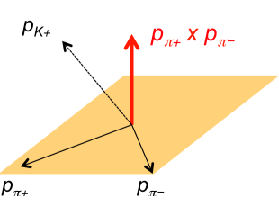
Figure 4: $T$-violating observable $p_{K^{+}}\cdot(p_{\pi^{+}}\times p_{\pi^{-}})$

The LHCb results are:

$$A_{T}(D^{0}) = (-71.8\,\pm 4.1\,\pm 1.3)\times 10^{-3}$$ (8)

$$\overline{A}_{T}(\overline{D}{}^{\,0}) = (-75.5\,\pm 4.1\,\pm 1.2)\times 10^{-3}$$ (9)

$$\Rightarrow\hskip 14.45377pta_{T} = (1.8\,\pm 2.9\,\pm 0.4)\times 10^{-3}\,.$$ (10)

Thus they see no evidence of $T$-violation. LHCb also calculates $a_{T}$ in 32 separate bins of phase space and in four bins of $D^{0}$ decay time. In both cases all values are consistent with zero. Fitting these values to a constant $a_{T}\!=\!0$ yields a $p$-value of 0.74 for the set of phase space measurements, and $p=0.83$ for the set of decay time measurements.

9 Mixing and $CP$ Violation

At this workshop, three recent measurements of mixing and $CP$ violation ($CPV$) parameters in the $D^{0}$-$\overline{D}{}^{\,0}$ system were presented: $y_{CP}$ by BESIII, $A_{\Gamma}$ by CDF, and $A_{\Gamma}$ by LHCb. These measurements are used by HFAG in their global fit for mixing and $CPV$ parameters $x,\,y,\,|q/p|$ and $\phi$, and are discussed below. In addition, CLEOc (Libby) showed evidence that the decay $D^{0}\!\rightarrow\!\pi^{+}\pi^{-}\pi^{0}$ is $CP$-even.

9.1 BESIII

BESIII (Albayrak) measures $y_{CP}\equiv(\Gamma_{CP+}-\Gamma_{CP-})/2\Gamma$, where $\Gamma=(\Gamma_{CP+}+\Gamma_{CP-})/2$, using semileptonic decays. Inverting this relation gives $\Gamma_{CP\pm}=\Gamma(1\pm y_{CP})$, and thus

$${\cal B}(CP+\,\!\rightarrow\!K\ell\nu) = \frac{\Gamma_{CP+\,\!\rightarrow\!K\ell\nu}}{\Gamma_{CP+}}\ =\ \frac{\Gamma_{CP+\,\!\rightarrow\!K\ell\nu}}{\Gamma(1+y_{CP})}\ \approx\ \frac{\Gamma_{CP+\,\!\rightarrow\!K\ell\nu}}{\Gamma}(1-y_{CP})\,.$$ (11)

Similarly, ${\cal B}(CP-\!\rightarrow\!K\ell\nu)\approx(\Gamma_{CP-\,\!\rightarrow\!K\ell\nu}/\Gamma)\times(1+y_{CP})$. Neglecting $CPV$ in $D^{0}$ decays, $\Gamma_{CP+\,\!\rightarrow\!K\ell\nu}=\Gamma_{CP-\,\!\rightarrow\!K\ell\nu}$ and one can show

$$y_{CP} \approx \frac{1}{4}\left(\frac{{\cal B}(CP-\!\rightarrow\!K\ell\nu)}{{\cal B}(CP+\!\rightarrow\!K\ell\nu)}-\frac{{\cal B}(CP+\!\rightarrow\!K\ell\nu)}{{\cal B}(CP-\!\rightarrow\!K\ell\nu)}\right)\,.$$ (12)

This method to determine $y_{CP}$ is advantageous as many systematic errors cancel in the ratio of branching fractions. The $CP$ of the decaying $D^{0}$ or $\overline{D}{}^{\,0}$ is identified by reconstructing the opposite-side $D$ decay in a $CP$-specific final state. The $CP$-even final states used are $K^{+}K^{-},\,\pi^{+}\pi^{-}$, and $K^{0}_{S}\,\pi^{0}\pi^{0}$; the $CP$-odd final states used are $K^{0}_{S}\,\pi^{0},\,K^{0}_{S}\,\omega$, and $K^{0}_{S}\,\eta$; and the semileptonic final states used are $K^{\pm}\mu^{\mp}\nu$ and $K^{\pm}e^{\mp}\nu$. The result of the measurement is $y_{CP}=(-2.0\,\pm 1.3\,\pm 0.7)$%. Although this result is less precise than that of other experiments using hadronic decays, it is the first such measurement using semileptonic decays, and the precision should improve with more data.

9.2 CDF

CDF (Leo) analyzes $CP$-even hadronic decays $D^{0}\!\rightarrow\!K^{+}K^{-},\,\pi^{+}\pi^{-}$ to measure the $CP$-violating parameter $A_{\Gamma}$. The observable used is the time-dependent $CP$ asymmetry

$$A_{CP}(t) \equiv \frac{N_{D^{0}}(t)-N_{\overline{D}{}^{\,0}}(t)}{N_{D^{0}}(t)+N_{\overline{D}{}^{\,0}}(t)}\ \approx\ A(0)-A_{\Gamma}\left(\frac{t}{\tau}\right)\,,$$ (13)

where the intercept $A(0)$ may be nonzero due to possible direct $CPV$ in the decay amplitude and any production or reconstruction asymmetries. By fitting the $A_{CP}(t)$ distribution to determine its slope, one obtains $A_{\Gamma}$. The CDF results are

$$A_{\Gamma}(KK) = (-1.9\,\pm 1.5\,\pm 0.4)\times 10^{-3}$$ (14)

$$A_{\Gamma}(\pi\pi) = (-0.1\,\pm 1.8\,\pm 0.3)\times 10^{-3}$$ (15)

$$\langle A_{\Gamma}\rangle = (-1.2\,\pm 1.2)\times 10^{-3}\,,$$ (16)

where the last result is a weighted average of the $K^{+}K^{-}$ and $\pi^{+}\pi^{-}$ results.

9.3 LHCb

LHCb (Reichert, Naik) measures $A_{\Gamma}$ using the same method as that used by CDF. The fit to the data is shown in Fig. 5. Due to the high statistics of the LHCb dataset, these results are the world’s most precise:

$$A_{\Gamma}(KK) = (-1.34\,\pm 0.77\,^{+0.26}_{-0.34})\times 10^{-3}$$ (17)

$$A_{\Gamma}(\pi\pi) = (-0.92\,\pm 1.45\,^{+0.25}_{-0.33})\times 10^{-3}\,.$$ (18)

Taking a weighted average of these values assuming the errors are uncorrelated gives

$$\langle A_{\Gamma}\rangle = (-1.24\,^{+0.71}_{-0.73})\times 10^{-3}\,.$$ (19)

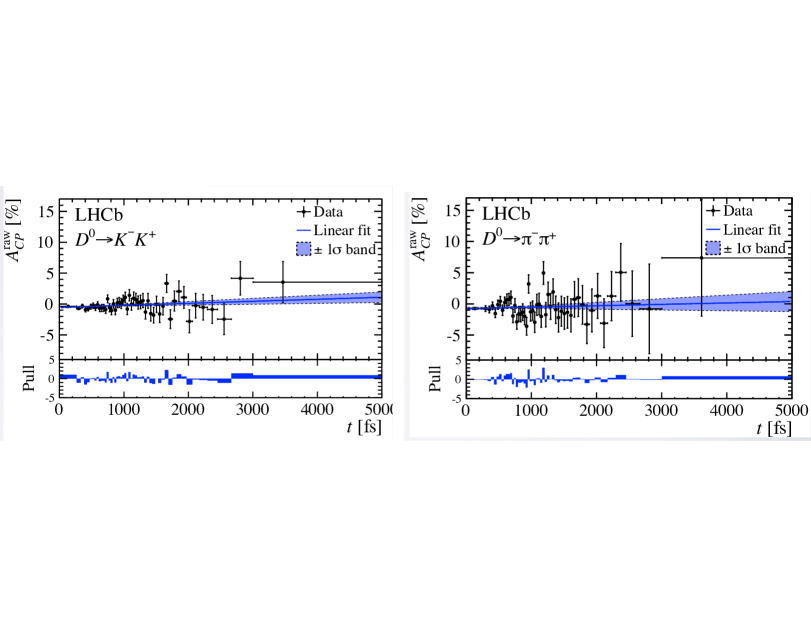
Figure 5: LHCb fit to the $D^{0}$ decay time distribution to determine $A_{\Gamma}$, using $D^{0}\!\rightarrow\!K^{+}K^{-}$ (left) and $D^{0}\!\rightarrow\!\pi^{+}\pi^{-}$ (right) decays.

9.4 Heavy Flavor Averaging Group Results

9.4.1 Global fit

HFAG performs a global fit to 45 observables measured from $D^{0}\!\rightarrow\!K^{+}\ell^{-}\nu$, $D^{0}\!\rightarrow\!K^{+}K^{-}$, $D^{0}\!\rightarrow\!\pi^{+}\pi^{-}$, $D^{0}\!\rightarrow\!K^{+}\pi^{-}$, $D^{0}\!\rightarrow\!K^{+}\pi^{-}\pi^{0}$, $D^{0}\!\rightarrow\!K^{0}_{S}\,\pi^{+}\pi^{-}$, and $D^{0}\!\rightarrow\!K^{0}_{S}\,K^{+}K^{-}$ decays, and from double-tagged branching fractions measured at the $\psi(3770)$ resonance. There are ten fitted parameters: mixing parameters $x$ and $y$; indirect $CPV$ parameters $|q/p|$ and $\phi$; the ratio of decay rates $R_{D}\equiv[\Gamma(D^{0}\!\rightarrow\!K^{+}\pi^{-})+\Gamma(\overline{D}{}^{\,0}\!\rightarrow\!K^{-}\pi^{+})]/[\Gamma(D^{0}\!\rightarrow\!K^{-}\pi^{+})+\Gamma(\overline{D}{}^{\,0}\!\rightarrow\!K^{+}\pi^{-})]$; direct $CPV$ parameters $A_{K}$, $A_{\pi}$, and $A_{D}=(R^{+}_{D}-R^{-}_{D})/(R^{+}_{D}+R^{-}_{D})$, where the $+\,(-)$ superscript corresponds to $D^{0}\,(\overline{D}{}^{\,0})$ decays; the strong phase difference $\delta$ between $\overline{D}{}^{\,0}\!\rightarrow\!K^{-}\pi^{+}$ and $D^{0}\!\rightarrow\!K^{-}\pi^{+}$ amplitudes; and the strong phase difference $\delta_{K\pi\pi}$ between $\overline{D}{}^{\,0}\!\rightarrow\!K^{-}\rho^{+}$ and $D^{0}\!\rightarrow\!K^{-}\rho^{+}$ amplitudes. The mixing parameters are defined as $x\equiv(m_{1}-m_{2})/\Gamma$ and $y\equiv(\Gamma_{1}-\Gamma_{2})/(2\Gamma)$, where $m_{1},\,m_{2}$ and $\Gamma_{1},\,\Gamma_{2}$ are the masses and decay widths for the $D^{0}$-$\overline{D}{}^{\,0}$ mass eigenstates, and $\Gamma=(\Gamma_{1}+\Gamma_{2})/2$. The fitter determines central values and errors using a $\chi^{2}$ statistic. Correlations among observables are accounted for by using covariance matrices provided by the experimental collaborations. Errors are assumed to be Gaussian. The relationships between observables and fitted parameters, and details of the fitting procedure, are given in Ref. [15].

All input measurements are given in Ref. [16]. The values for observables $R_{M}=(x^{2}+y^{2})/2$, $y_{CP}$, and $\Gamma_{CP}$ are world averages as calculated by HFAG [17]. For the latter two observables, the world averages used include the results presented by BESIII and LHCb at this workshop (see Fig. 6).

   

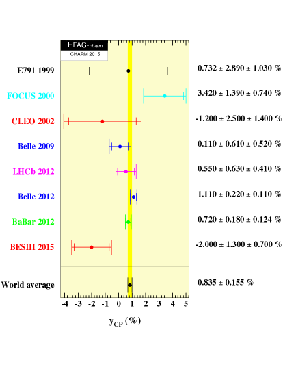
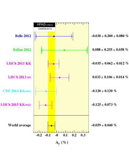
Figure 6: World average values for $y_{CP}$ (left) and $A_{\Gamma}$ (right) as calculated by HFAG [17]. These values include the results from BESIII and LHCb presented at this workshop.

Four types of fits are performed: (a) assuming $CP$ conservation (fixing $A_{D}\!=\!0$, $A_{K}\!=\!0$, $A_{\pi}\!=\!0$, $\phi\!=\!0$, and $|q/p|\!=\!1$); (b) assuming no direct $CPV$ in doubly Cabibbo-suppressed (DCS) decays, which fixes $A_{D}\!=\!0$ and reduces the four independent parameters $(x,y,|q/p|,\phi)$ to three via the relation $\tan\phi=(1-|q/p|^{2})/(1+|q/p|^{2})\times(x/y)$ [18, 19]; (c) same as fit (b) except that one fits for alternative parameters $x_{12}=2|M_{12}|/\Gamma$, $y_{12}=\Gamma_{12}/\Gamma$, and $\phi_{12}={\rm Arg}(M_{12}/\Gamma_{12})$, where $M_{12}$ and $\Gamma_{12}$ are the off-diagonal elements of the $D^{0}$-$\overline{D}{}^{\,0}$ mass and decay matrices, respectively; and (d) allowing full $CPV$ (floating all parameters). Note that parameters $(x_{12},\,y_{12},\,\phi_{12})$ can be derived from $(x,\,y,\,|q/p|,\,\phi)$ and vice-versa; see Ref. [16].

All fit results are listed in Table 7, and two-dimensional contour plots are shown in Fig. 7 (no-direct-$CPV$) and Fig. 8 (all-$CPV$-allowed). These results show that $D^{0}$ mesons mix: the no-mixing point $x=y=0$ is excluded at $>12\sigma$. There is no evidence for $CPV$ arising from $D^{0}$-$\overline{D}{}^{\,0}$ mixing ($|q/p|\neq 1$) or from a phase difference between the mixing amplitude and a direct decay amplitude ($\phi\neq 0$).

   

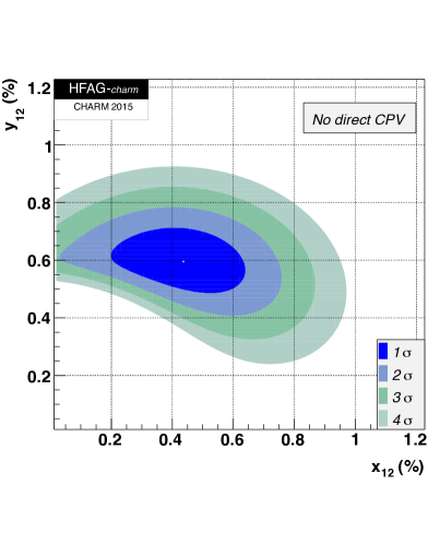
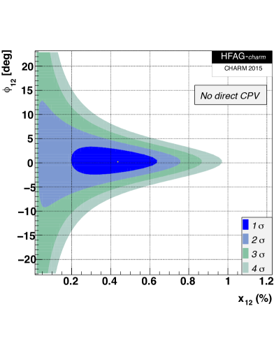
Figure 7: Two-dimensional contour plots for parameters $(x_{12},y_{12})$ (top left), $(x_{12},\phi_{12})$ (top right), and $(y_{12},\phi_{12})$ (bottom) for no direct $CPV$ in DCS decays, as calculated by HFAG [16].

   

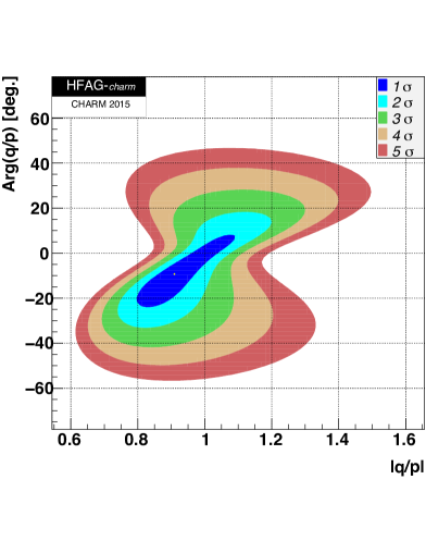
Figure 8: Two-dimensional contour plots for parameters $(x,y)$ (left) and $(|q/p|,\phi)$ (right), allowing for $CPV$, as calculated by HFAG [16].

Parameter	No $CPV$	No direct $CPV$	$CPV$-allowed	95% C.L. Interval
		in DCS decays
$\begin{array}[]{c}x\ (\%)\\ y\ (\%)\\ \delta_{K\pi}\ (^{\circ})\\ R_{D}\ (\%)\\ A_{D}\ (\%)\\ |q/p|\\ \phi\ (^{\circ})\\ \delta_{K\pi\pi}\ (^{\circ})\\ A_{\pi}\\ A_{K}\\ x_{12}\ (\%)\\ y_{12}\ (\%)\\ \phi_{12}(^{\circ})\end{array}$	$\begin{array}[]{c}0.49\,^{+0.14}_{-0.15}\\ 0.61\,\pm 0.08\\ 6.9\,^{+9.7}_{-11.2}\\ 0.349\,\pm 0.004\\ -\\ -\\ -\\ 18.1\,^{+23.3}_{-23.8}\\ -\\ -\\ -\\ -\\ -\end{array}$	$\begin{array}[]{c}0.44\,^{+0.14}_{-0.15}\\ 0.60\,\pm 0.07\\ 3.6\,^{+10.4}_{-12.1}\\ 0.348\,\pm 0.004\\ -\\ 1.002\,\pm 0.014\\ -0.07\,\pm 0.6\\ 20.3\,^{+24.0}_{-24.3}\\ 0.10\,\pm 0.14\\ -0.14\,\pm 0.13\\ 0.44\,^{+0.14}_{-0.15}\\ 0.60\,\pm 0.07\\ 0.2\,\pm 1.7\end{array}$	$\begin{array}[]{c}0.37\,\pm 0.16\\ 0.66\,\,^{+0.07}_{-0.10}\\ 11.8\,^{+9.5}_{-14.7}\\ 0.349\,\pm 0.004\\ -0.39\,^{+1.01}_{-1.05}\\ 0.91\,^{+0.12}_{-0.08}\\ -9.4\,^{+11.9}_{-9.8}\\ 27.3\,^{+24.4}_{-25.4}\\ 0.10\,\pm 0.15\\ -0.15\,\pm 0.14\\ \\ \\ \\ \end{array}$	$\begin{array}[]{c}\left[0.06,\,0.67\right]\\ \left[0.46,\,0.79\right]\\ \left[-21.1,\,29.3\right]\\ \left[0.342,\,0.357\right]\\ \left[-2.4,\,1.5\right]\\ \left[0.77,\,1.14\right]\\ \ \left[-28.3,\,12.9\right]\\ \left[-23.3,\,74.8\right]\\ \left[-0.19,\,0.38\right]\\ \left[-0.42,\,0.12\right]\\ \left[0.13,\,0.69\right]\\ \left[0.45,\,0.74\right]\\ \left[-4.1,\,4.6\right]\\ \end{array}$

Table 7: Results of the HFAG global fit for mixing and $CPV$ parameters [16]. The most recent results for $y_{CP}$ and $A_{\Gamma}$ are used in the fit.

9.4.2 Dedicated fit for $CPV$ parameters

HFAG also performs a fit for alternative direct and indirect $CPV$ parameters $a^{\rm dir}_{CP}$ and $a^{\rm ind}_{CP}$. The observables are

$$A_{\Gamma} \equiv \frac{\tau(\overline{D}{}^{\,0}\!\rightarrow\!h^{+}h^{-})-\tau(D^{0}\!\rightarrow\!h^{+}h^{-})}{\tau(\overline{D}{}^{\,0}\!\rightarrow\!h^{+}h^{-})+\tau(D^{0}\!\rightarrow\!h^{+}h^{-})}\,,$$ (20)

where $h^{+}h^{-}$ is either $K^{+}K^{-}$ or $\pi^{+}\pi^{-}$; and $\Delta A_{CP}\equiv A_{CP}(K^{+}K^{-})-A_{CP}(\pi^{+}\pi^{-})$, where $A_{CP}$ are time-integrated $CP$ asymmetries. The relations between the observables and the fitted parameters are [20]:

$$A_{\Gamma} = -a^{\rm ind}_{CP}-a^{\rm dir}_{CP}\,y_{CP}$$ (21)

$$\Delta A_{CP} = \Delta a^{\rm dir}_{CP}\left(1+y_{CP}\frac{\overline{\langle t\rangle}}{\tau}\right)+a^{\rm ind}_{CP}\frac{\Delta\langle t\rangle}{\tau}+\overline{a}^{\rm\,dir}_{CP}\,y_{CP}\frac{\Delta\langle t\rangle}{\tau}$$ (22)

$$\approx \Delta a^{\rm dir}_{CP}\left(1+y_{CP}\frac{\overline{\langle t\rangle}}{\tau}\right)+a^{\rm ind}_{CP}\frac{\Delta\langle t\rangle}{\tau}\,.$$

In the second relation, $\langle t\rangle/\tau$ denotes the mean decay time in units of $D^{0}$ lifetime; $\Delta X$ denotes the difference in quantity $X$ between $K^{+}K^{-}$ and $\pi^{+}\pi^{-}$ final states; and $\overline{X}$ denotes the average for quantity $X$. HFAG uses values of $\overline{\langle t\rangle}$ and $\Delta\langle t\rangle$ specific to each experiment, and the observables $A_{\Gamma}(KK)$ and $A_{\Gamma}(\pi\pi)$ are assumed to be identical. The measurements used and details of the fit are given in Ref. [21]. Parameters $a^{\rm dir}_{CP}(K^{+}K^{-})$ and $a^{\rm dir}_{CP}(\pi^{+}\pi^{-})$ are expected to have opposite signs [22].

The fit results are shown in Fig. 9, which plots all relevant measurements in the two-dimensional $(a^{\rm ind}_{CP},\Delta a^{\rm dir}_{CP})$ plane. The most likely values and $\pm 1\sigma$ errors are [21]:

$$a^{\rm ind}_{CP} = (+0.058\pm 0.040)\%$$ (23)

$$\Delta a^{\rm dir}_{CP} = (-0.257\pm 0.104)\%\,.$$ (24)

Whereas $a^{\rm ind}_{CP}$ is consistent with zero, $\Delta a^{\rm dir}_{CP}$ is not. The two-dimensional significance is $2.0\sigma$, and thus the data is inconsistent with $CP$ conservation at this level.

Figure 9: HFAG fit for parameters $a^{\rm dir}_{CP}$ and $a^{\rm ind}_{CP}$ [21]. Measurements are plotted as bands showing their $\pm 1\sigma$ range. The no-$CPV$ point (0,0) is shown as a filled circle, and the best fit value is indicated by a cross showing the one-dimensional errors.

ACKNOWLEDGEMENTS

We are grateful to the organizers of CHARM 2015 for an enjoyable and productive workshop.

References

- [1] Throughout this paper, charge-conjugate modes are implicitly included unless stated or implied otherwise.
- [2] CMS Collaboration, CMS PAS HIN-12-014 (August, 2012).
- [3] X. L. Wang et al. (Belle Collaboration), Phys. Rev. D 91, 112007 (2015).
- [4] Z. Q. Liu et al. (Belle Collaboration), Phys. Rev. Lett. 110, 252002 (2013).
- [5] X. L. Wang et al. (Belle Collaboration), Phys. Rev. D 87, 051101(R) (2013).
- [6] E. M. Aitala et al. (FNAL E791 Collaboration), Phys. Rev. D 73, 032004 (2006).
- [7] R. Aaij et al. (LHCb Collaboration), Phys. Rev. D 91, 092002 (2015).
- [8] J. Beringer et al. (Particle Data Group), Phys. Rev. D 86, 010001 (2012).
- [9] S. Aoki et al., Eur. Phys. Jour. C 74, 2890 (2014).
- [10] www.slac.stanford.edu/xorg/hfag/charm/Vcd/december14/results.html.
- [11] www.slac.stanford.edu/xorg/hfag/charm/Vcs/december14/results.html.
- [12] J. P. Lees et al. (BaBar Collaboration), Phys. Rev. D 85, 091107 (2012).
- [13] M. Ablikim et al. (BESIII Collaboration), Phys. Rev. D 91, 112015 (2015).
- [14] www.slac.stanford.edu/xorg/hfag/charm/cp_asym/charm_todd_asym_8feb15.html.
- [15] Y. Amhis et al. (Heavy Flavor Averaging Group), arXiv:1412.7515 (2014).
- [16] www.slac.stanford.edu/xorg/hfag/charm/CHARM15/results_mix_cpv.html.
- [17] www.slac.stanford.edu/xorg/hfag/charm/CHARM15/results_mixing.html.
- [18] M. Ciuchini et al., Phys. Lett. B 655, 162 (2007).
- [19] A. Kagan and M. Sokoloff, Phys. Rev. D 80, 076008 (2009).
- [20] M. Gersabeck et al., J. Phys. G 39, 045005 (2012).
- [21] www.slac.stanford.edu/xorg/hfag/charm/April15/DCPV/direct_indirect_cpv.html
- [22] Y. Grossman, A. L. Kagan, and Y. Nir, Phys. Rev. D 75, 036008 (2007).