An Iterative Reweighted Method for Tucker Decomposition of Incomplete Multiway Tensors

Abstract

We consider the problem of low-rank decomposition of incomplete multiway tensors. Since many real-world data lie on an intrinsically low dimensional subspace, tensor low-rank decomposition with missing entries has applications in many data analysis problems such as recommender systems and image inpainting. In this paper, we focus on Tucker decomposition which represents an $N$th-order tensor in terms of $N$ factor matrices and a core tensor via multilinear operations. To exploit the underlying multilinear low-rank structure in high-dimensional datasets, we propose a group-based log-sum penalty functional to place structural sparsity over the core tensor, which leads to a compact representation with smallest core tensor. The method for Tucker decomposition is developed by iteratively minimizing a surrogate function that majorizes the original objective function, which results in an iterative reweighted process. In addition, to reduce the computational complexity, an over-relaxed monotone fast iterative shrinkage-thresholding technique is adapted and embedded in the iterative reweighted process. The proposed method is able to determine the model complexity (i.e. multilinear rank) in an automatic way. Simulation results show that the proposed algorithm offers competitive performance compared with other existing algorithms.

I Introduction

Multi-dimensional data arise in a variety of applications, such as recommender systems [1, 2, 3], multirelational networks [4, 5], and brain-computer imaging [6, 7]. Tensors (i.e. multiway arrays) provide an effective representation of such data. Tensor decomposition based on low rank approximation is a powerful technique to extract useful information from multiway data as many real-world multiway data are lying on a low dimensional subspace. Compared with matrix factorization, tensor decomposition can capture the intrinsic multi-dimensional structure of the multiway data, which has led to a substantial performance improvement for harmonic retrieval [8, 9], regression/classification [10, 11, 12], and data completion [3, 13], etc. Tucker decomposition [14] and CANDECOMP/PARAFAC (CP) decomposition [15] are two widely used low-rank tensor decompositions. Specifically, CP decomposes a tensor as a sum of rank-one tensors, whereas Tucker is a more general decomposition which involves multilinear operations between a number of factor matrices and a core tensor. CP decomposition can be viewed as a special case of Tucker decomposition with a super-diagonal core tensor. It is generally believed that Tucker decomposition has a better generalization ability than CP decomposition for different types of data [16]. In many applications, only partial observations of the tensor may be available. It is therefore important to develop efficient tensor decomposition methods for incomplete, sparsely observed data where a significant fraction of entries is missing.

Low-rank decomposition of incomplete multiway tensors has attracted a lot of attention over the past few years and a number of algorithms [17, 18, 19, 20, 21, 22, 23, 24, 25, 26, 27, 28] were proposed via either optimization techniques or probabilistic model learning. For both CP and Tucker decompositions, the most challenging task is to determine the model complexity (i.e. the rank of the tensor) in the presence of missing entries and noise. It has been shown that determining the CP rank, i.e. the minimum number of rank-one terms in CP decomposition, is an NP-hard problem even for a completely observed tensor [29]. Unfortunately, many existing methods require that the rank of the decomposition is specified a priori. To address this issue, a Bayesian method was proposed in [13] for CP decomposition, where a shrinkage prior called as the multiplicative gamma process (MGP) was employed to adaptively learn a concise representation of the tensor. In [26], a sparsity-inducing Gaussian inverse-Gamma prior was placed over multiple latent factors to achieve automatic rank determination. Besides the above Bayesian methods, an optimization-based CP decomposition method was proposed in [18, 19], where the Frobenius-norm of the factor matrices is used as the rank regularization to determine an appropriate number of component tensors.

In addition to the CP rank, another notion of tensor rank is multilinear rank [30], which is defined as the tuple of the ranks of the mode-$n$ unfoldings of the tensor. Multilinear rank is closely related to the Tucker decomposition since the multilinear rank is equivalent to the dimension of the smallest achievable core tensor in Tucker decomposition [31]. To search for a low multilinear rank representation, a tensor nuclear norm, defined as a (weighted) summation of nuclear norms of mode-$n$ unfoldings, was introduced to approximate the multilinear rank. Tensor completion and decomposition can then be accomplished by minimizing the tensor nuclear norm. Specifically, an alternating direction method of multipliers (ADMM) was developed in [17, 23] to minimize the tensor nuclear norm with missing data, and encouraging results were reported on visual data. The success of [17] has inspired a number of subsequent works [21, 22, 32, 33, 24, 25] for tensor completion and decomposition based on tensor nuclear norm minimization. Nevertheless, the tensor nuclear norm, albeit effective, is not necessarily the tightest convex envelope of the multilinear rank [21]. Also, the nuclear norm-based methods are sensitive to outliers and work well only if the tensor is exactly low multilinear rank.

In this paper, to automatically achieve a concise Tucker representation, we introduce a notion referred to as the order-$(N-1)$ sub-tensor and propose a group log-sum penalty functional to encourage structural sparsity of the core tensor. Specifically, in the log-sum penalty function, elements in every sub-tensor of the core tensor along each mode are grouped together. Minimizing the group log-sum penalty function thus leads to a structured sparse core tensor with only a few nonzero order-$(N-1)$ sub-tensors along each mode. By removing the zero order-$(N-1)$ sub-tensors, the core tensor shrinks and a compact Tucker decomposition can be obtained. Note that the log-sum function which behaves like the $\ell_{0}$-norm is more sparsity-encouraging than the nuclear norm that is $\ell_{1}$-norm applied to the singular values of a matrix. Thus we expect the group log-sum minimization is more effective than the tensor nuclear norm-minimization in finding a concise representation of the tensor. By resorting to a majorization-minimization approach, we develop an iterative reweighted method via iteratively decreasing a surrogate function that majorizes the original log-sum penalty function. The proposed method can determine the model complexity (i.e. multilinear rank) in an automatic way. Also, the over-relaxed monotone fast iterative shrinkage-thresholding technique [34] is adapted and embedded in the iterative reweighted process, which achieves a substantial reduction in computational complexity.

The remainder of this paper is organized as follows. Section II provides notations and basics on tensors. The problem of Tucker decomposition with incomplete entries is formulated as an unconstrained optimization problem in Section III. An iterative reweighted method is developed in Section IV for Tucker decomposition of incomplete multiway tensors. In Section V, the over-relaxed monotone fast iterative shrinkage-thresholding technique is adapted and integrated with the proposed iterative reweighted method, which results in a significant computational complexity reduction. Simulation results are provided in section VI, followed by concluding remarks in Section VII.

II Notations and Basics on Tensors

We first provide a brief review on tensor decompositions. A tensor is the generalization of a matrix to higher dimensions, also known as ways or modes. Vectors and matrices can be viewed as special cases of tensors with one and two modes, respectively. Throughout this paper, we use symbols $\otimes$ , $\circ$ and $\ast$ to denote the Kronecker, outer and Hadamard product, respectively.

Let $\boldsymbol{\mathcal{X}}\in\mathbb{R}^{I_{1}\times I_{2}\times\cdots\times I_{N}}$ denote an $N$th order tensor with its $(i_{1},\ldots,i_{N})$th entry denoted by $\mathcal{X}_{i_{1}\cdots i_{N}}$. Here the order $N$ of a tensor is the number of dimensions. Fibers are the higher-order analogue of matrix rows and columns. The mode-$n$ fibers of $\boldsymbol{\mathcal{X}}$ are $I_{n}$-dimensional vectors obtained by fixing every index but $i_{n}$. Slices are two-dimensional sections of a tensor, defined by fixing all but two indices. Unfolding or matricization is an operation that turns a tensor into a matrix. Specifically, the mode-$n$ unfolding of a tensor $\boldsymbol{\mathcal{X}}$, denoted as $\boldsymbol{X}_{(n)}$, arranges the mode-$n$ fibers to be the columns of the resulting matrix. For notational convenience, we also use the notation $\textrm{unfold}_{n}(\boldsymbol{\mathcal{X}})$ to denote the unfolding operation along the $n$-th mode. The $n$-mode product of $\boldsymbol{\mathcal{X}}$ with a matrix $\boldsymbol{A}\in\mathbb{R}^{J\times I_{n}}$ is denoted by $\boldsymbol{\mathcal{X}}\times_{n}\boldsymbol{A}$ and is of size $I_{1}\cdots\times I_{n-1}\times J\times I_{n+1}\times\cdots\times I_{N}$, with each mode-$n$ fiber multiplied by the matrix $\boldsymbol{A}$, i.e.

$$\boldsymbol{\mathcal{Y}}=\boldsymbol{\mathcal{X}}\times_{n}\boldsymbol{A}\Leftrightarrow\boldsymbol{Y}_{(n)}=\boldsymbol{A}\boldsymbol{X}_{(n)}$$ (1)

The CP decomposition decomposes a tensor into a sum of rank-one component tensors, i.e.

$$\boldsymbol{\mathcal{X}}=\sum\limits_{r=1}^{R}\lambda_{r}\boldsymbol{a}_{r}^{(1)}\circ\boldsymbol{a}_{r}^{(2)}\circ\cdots\circ\boldsymbol{a}_{r}^{(N)}$$ (2)

where $\boldsymbol{a}_{r}^{(n)}\in\mathbb{R}^{I_{n}}$, ‘$\circ$’ denotes the vector outer product, and $R$ is referred to as the rank of the tensor. Elementwise, we have

$$\mathcal{X}_{i_{1}i_{2}\cdots i_{N}}=\sum\limits_{r=1}^{R}\lambda_{r}a_{i_{1}r}^{(1)}a_{i_{2}r}^{(2)}\cdots a_{i_{N}r}^{(N)}$$ (3)

The Tucker decomposition can be considered as a high order principle component analysis. It decomposes a tensor into a core tensor multiplied by a factor matrix along each mode. The Tucker decomposition of an $N$-th order tensor $\boldsymbol{\mathcal{X}}$ can be written as

$$\boldsymbol{\mathcal{X}} =\boldsymbol{\mathcal{G}}\times_{1}\boldsymbol{A}^{(1)}\times_{2}\boldsymbol{A}^{(2)}\cdots\times_{N}\boldsymbol{A}^{(N)}$$

$$=\sum\limits_{r_{1}=1}^{R_{1}}\sum\limits_{r_{2}=2}^{R_{2}}\cdots\sum\limits_{r_{N}=1}^{R_{N}}\mathcal{G}_{r_{1}r_{2}\cdots r_{N}}\boldsymbol{a}^{(1)}_{r_{1}}\circ\boldsymbol{a}^{(2)}_{r_{2}}\circ\cdots\circ\boldsymbol{a}^{(N)}_{r_{N}}$$ (4)

where $\boldsymbol{\mathcal{G}}\in\mathbb{R}^{R_{1}\times R_{2}\times\cdots\times R_{N}}$ is the core tensor, and $\boldsymbol{A}^{(n)}\triangleq[\boldsymbol{a}_{1}^{(n)}\phantom{0}\ldots\phantom{0}\boldsymbol{a}_{R_{n}}^{(n)}]\in\mathbb{R}^{I_{n}\times R_{n}}$ denotes the factor matrix along the $n$-th mode (see Fig.1).

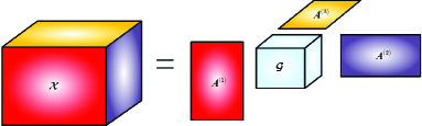
Figure 1: The Tucker decomposition of a three-order tensor.

The inner product of two tensors with the same size is defined as

$$\langle\boldsymbol{\mathcal{X}},\boldsymbol{\mathcal{Y}}\rangle=\sum\limits_{i_{1}=1}^{I_{1}}\sum\limits_{i_{2}=1}^{I_{2}}\cdots\sum\limits_{i_{N}=1}^{I_{N}}x_{i_{1}i_{2}\dots i_{N}}y_{i_{1}i_{2}\dots i_{N}}$$ (5)

The Frobenius norm of a tensor $\boldsymbol{\mathcal{X}}$ is square root of the inner product with itself, i.e.

$$\|\boldsymbol{\mathcal{X}}\|_{F}=\langle\boldsymbol{\mathcal{X}},\boldsymbol{\mathcal{X}}\rangle^{\frac{1}{2}}$$ (6)

Also, for notational convenience, the sequential Kronecker product of a set of matrices in a reversed order is defined and denoted by

$$\bigotimes_{n}\boldsymbol{A}^{(n)}=\boldsymbol{A}^{(N)}\otimes\boldsymbol{A}^{(N-1)}\otimes\cdots\otimes\boldsymbol{A}^{(1)}$$

$$\bigotimes_{n\neq k}\boldsymbol{A}^{(n)}=\boldsymbol{A}^{(N)}\otimes\cdots\otimes\boldsymbol{A}^{(k+1)}\otimes\boldsymbol{A}^{(k-1)}\otimes\cdots\otimes\boldsymbol{A}^{(1)}$$

An $N$th order tensor $\boldsymbol{\mathcal{X}}$ multiplied by factor matrices $\{\boldsymbol{A}^{(k)}\}_{k=1}^{N}$ along each mode is denoted by

$$\boldsymbol{\mathcal{X}}\prod\limits_{n=1}^{N}\times_{n}\boldsymbol{A}^{(n)}=\boldsymbol{\mathcal{X}}\times_{1}\boldsymbol{A}^{(1)}\times_{2}\boldsymbol{A}^{(2)}\cdots\times_{N}\boldsymbol{A}^{(N)},$$

while the tensor $\boldsymbol{\mathcal{X}}$ multiplied by the factor matrices along every mode except the $k$-th mode is denoted as

$$\boldsymbol{\mathcal{X}}\prod\limits_{n\neq k}\times_{n}\boldsymbol{A}^{(n)}=\boldsymbol{\mathcal{X}}\times_{1}\boldsymbol{A}^{(1)}\cdots\times_{k-1}\boldsymbol{A}^{(k-1)}$$

$$\qquad\qquad\qquad\qquad\qquad\qquad\times_{k+1}\boldsymbol{A}^{(k+1)}\cdots\times_{N}\boldsymbol{A}^{(N)}.$$

With these notations, vectorization and unfolding of a tensor which admits a Tucker decomposition (4) can be expressed as

$$\text{vec}(\boldsymbol{\mathcal{X}})=\Big{(}\bigotimes_{n}\boldsymbol{A}^{(n)}\Big{)}\text{vec}(\boldsymbol{\mathcal{G}})$$ (7)

$$\text{unfold}_{n}(\boldsymbol{\mathcal{X}})=\boldsymbol{A}^{(n)}\boldsymbol{G}_{(n)}\Big{(}\bigotimes_{k\neq n}\boldsymbol{A}^{(k)}\Big{)}^{T}$$ (8)

III Problem Formulation

Let $\boldsymbol{\mathcal{Y}}\in\mathbb{R}^{I_{1}\times I_{2}\times\cdots\times I_{N}}$ be an incomplete $N$th order tensor, with its entry $\mathcal{Y}_{i_{1}i_{2}\dots i_{N}}$ observed if $\mathcal{O}_{i_{1}i_{2}\dots i_{N}}=1$, where $\boldsymbol{\mathcal{O}}\in\{0,1\}^{I_{1}\times I_{2}\times\cdots\times I_{N}}$ is a binary tensor of the same size as $\boldsymbol{\mathcal{Y}}$ and indicates which entries of $\boldsymbol{\mathcal{Y}}$ are missing or observed. Given the observed data, our objective is to find a Tucker decomposition which has a minimum model complexity and meanwhile fits the observed data, or to be more precise, seek a Tucker representation such that the data can be represented by a smallest core tensor. Since the dimension of the smallest achievable core tensor is unknown a priori, we need to develop a method that can achieve automatic model determination. To this objective, we first introduce a new notion called as order-$(N-1)$ sub-tensor.

Definition: Order-$(N-1)$ sub-tensor is defined as a new tensor obtained by fixing only one index of the original tensor. Let $\boldsymbol{\mathcal{Z}}\in\mathbb{R}^{I_{1}\times I_{2}\times\cdots\times I_{N}}$ be an $N$th order tensor. The $i$th $(1\leq i\leq I_{n})$ sub-tensor along the $n$th mode of $\boldsymbol{\mathcal{Z}}$, denoted as $\boldsymbol{\mathcal{Z}}_{(n,i)}$, is an $(N-1)$th order tensor of size $I_{1}\times I_{2}\times\cdots I_{n-1}\times I_{n+1}\cdots\times I_{N}$, and its $(j_{1},\ldots,j_{N-1})$th entry are given by $\mathcal{X}_{j_{1},\ldots,j_{n-1},i,j_{n+1},\ldots,j_{N-1}}$. For tensors with three modes, i.e. $N=3$, order-$(N-1)$ sub-tensors reduce to slices, although order-$(N-1)$ sub-tensors are generally different from slices.

Clearly, $\boldsymbol{\mathcal{Z}}$ consists of $I_{n}$ order-$(N-1)$ sub-tensors along its $n$th mode. If some order-$(N-1)$ sub-tensors along the $n$th mode become zero, then the dimension of $\boldsymbol{\mathcal{Z}}$ along the $n$th mode is reduced accordingly. Suppose the data tensor $\boldsymbol{\mathcal{Y}}$ has a Tucker decomposition

$$\boldsymbol{\mathcal{Y}}=\boldsymbol{\mathcal{X}}\prod\limits_{n=1}^{N}\times_{n}\boldsymbol{A}^{(n)}$$ (9)

Unfolding $\boldsymbol{\mathcal{Y}}$ along the $n$th mode, we have

$$\boldsymbol{Y}_{(n)}= \boldsymbol{A}^{(n)}\boldsymbol{X}_{(n)}\Big{(}\bigotimes_{k\neq n}\boldsymbol{A}^{(k)}\Big{)}^{T}$$

$$= \sum\limits_{i=1}^{I_{n}}\boldsymbol{a}^{(n)}_{\cdot,i}\boldsymbol{x}^{(n)}_{i,\cdot}\Big{(}\bigotimes_{k\neq n}\boldsymbol{A}^{(k)}\Big{)}^{T}$$ (10)

where $\boldsymbol{a}^{(n)}_{\cdot,i}$ is the $i$th column of $\boldsymbol{A}^{(n)}$ and $\boldsymbol{x}^{(n)}_{i,\cdot}$ is the $i$th row of $\boldsymbol{X}_{(n)}$. Clearly, $\boldsymbol{x}^{(n)}_{i,\cdot}$ is the vectorization of the $i$th order $(N-1)$ sub-tensor along the $n$th mode. If $\boldsymbol{x}^{(n)}_{i,\cdot}$ is a zero vector, i.e. the corresponding order-$(N-1)$ sub-tensor is a zero tensor, both $\boldsymbol{a}^{(n)}_{\cdot,i}$ and $\boldsymbol{x}^{(n)}_{i,\cdot}$ have no contribution to $\boldsymbol{\mathcal{Y}}$ and can thus be removed. Inspired by this insight, sparsity can be enforced over each sub-tensor (along each mode) of the core tensor such that the observed data can be represented by a structural sparsest core tensor with only a few nonzero sub-tensors over all modes. By removing those zero sub-tensors along each mode (the associated columns of the factor matrices are disabled and can be removed as well), the core tensor shrinks to a smaller one and a compact Tucker decomposition can be obtained. The problem can be formulated as

$$\min_{\boldsymbol{\mathcal{X}},\{\boldsymbol{A}^{(n)}\}} \quad\sum\limits_{n=1}^{N}\|\boldsymbol{z}_{n}\|_{0}$$

s.t. $$\quad\|\boldsymbol{\mathcal{O}}\ast(\boldsymbol{\mathcal{Y}}-\boldsymbol{\mathcal{X}}\prod\limits_{n=1}^{N}\times_{n}\boldsymbol{A}^{(n)})\|_{F}^{2}\leq\varepsilon$$ (11)

where $\varepsilon$ is an error tolerance parameter related to noise statistics, and $\boldsymbol{z}_{n}$ is an $I_{n}$-dimensional vector with its $i$th entry given by

$$z_{n,i}\triangleq\|\boldsymbol{\mathcal{X}}_{(n,i)}\|_{F}$$ (12)

It should be noted that since there is usually no knowledge about the size of smallest core tensor, the dimensions of the core tensor are predefined to be the same as the original tensor, i.e. $\boldsymbol{\mathcal{X}}\in\mathbb{R}^{I_{1}\times I_{2}\times\cdots\times I_{N}}$. The term $\|\boldsymbol{z}_{n}\|_{0}$ specifies the number of nonzero sub-tensors along the $n$th mode of tensor $\boldsymbol{\mathcal{X}}$. Since the number of nonzero sub-tensors along the $n$th mode is equivalent to the dimension of mode-$n$ of the core tensor, the above optimization yields a smallest (in terms of sum of dimensions of all modes) core tensor. The optimization (11), however, is an NP-hard problem. Thus, alternative sparsity-promoting functions which are more computationally efficient in finding the structural sparse core tensor are desirable. In this paper, we consider the use of the log-sum sparsity-encouraging functional. Log-sum penalty function has been extensively used for sparse signal recovery and was shown to be more sparsity-encouraging than the $\ell_{1}$-norm [35, 36, 37, 38]. Replacing the $\ell_{0}$-norm in (11) with the log-sum functional leads to

$$\min_{\boldsymbol{\mathcal{X}},\{\boldsymbol{A}^{(n)}\}}\quad \sum\limits_{n=1}^{N}\sum\limits_{i=1}^{I_{n}}\log(\|\boldsymbol{\mathcal{X}}_{(n,i)}\|_{F}^{2}+\epsilon)$$

s.t. $$\|\boldsymbol{\mathcal{O}}\ast(\boldsymbol{\mathcal{Y}}-\boldsymbol{\mathcal{X}}\prod\limits_{n=1}^{N}\times_{n}\boldsymbol{A}^{(n)})\|_{F}^{2}\leq\varepsilon$$ (13)

where $\epsilon$ is a small positive parameter to ensure the logarithmic function is well-defined. Note that in our formulation, coefficients are grouped according to sub-tensors and different sub-tensors may have overlapping entries. This is different from the group-LASSO [39, 40] method in which entries are grouped into a number of non-overlapping subsets with sparsity imposed on each subset. Also, to avoid the solution $\boldsymbol{\mathcal{X}}\to 0$ and $\{\boldsymbol{A}^{(n)}\}\to\infty$, a Frobenius norm can be imposed on the factor matrices $\{\boldsymbol{A}^{(n)}\}$. The optimization (13) can eventually be formulated as an unconstrained optimization problem as follows

$$\min_{\boldsymbol{\mathcal{X}},\{\boldsymbol{A}^{(n)}\}} L(\boldsymbol{\mathcal{X}},\{\boldsymbol{A}^{(n)}\})=\sum\limits_{n=1}^{N}\sum\limits_{i=1}^{I_{n}}\log(\|\boldsymbol{\mathcal{X}}_{(n,i)}\|_{F}^{2}+\epsilon)$$

$$+\lambda_{1}\Big{\|}\boldsymbol{\mathcal{O}}\ast\Big{(}\boldsymbol{\mathcal{Y}}-\boldsymbol{\mathcal{X}}\prod\limits_{n=1}^{N}\times_{n}\boldsymbol{A}^{(n)}\Big{)}\Big{\|}_{F}^{2}+\lambda_{2}\sum\limits_{n=1}^{N}\|\boldsymbol{A}^{(n)}\|_{F}^{2}$$ (14)

where $\lambda_{1}$ is a parameter controlling the tradeoff between the sparsity of the core tensor and the fitting error, and $\lambda_{2}$ is a regularization parameter for factor matrices. Their choices will be discussed later in our paper.

The above optimization (14) can be viewed as searching for a low multilinear rank representation of the observed data. Multilinear rank, also referred to as $n$-rank, of an $N$-order tensor $\boldsymbol{\mathcal{X}}$ is defined as the tuple of the ranks of the mode-$n$ unfoldings, i.e.

$$\text{$n$-rank}\triangleq\{\text{rank}(\boldsymbol{X}_{(1)}),\text{rank}(\boldsymbol{X}_{(2)}),\ldots,\text{rank}(\boldsymbol{X}_{(N)})\}$$ (15)

It can be shown that $n$-rank is equivalent to the dimensions of the smallest achievable core tensor in Tucker decomposition[31]. Therefore the optimization (14) can also be used for recovery of incomplete low $n$-rank tensors. Existing methods for low $n$-rank completion employ a tensor nuclear-norm, defined as a (weighted) summation of nuclear-norms of mode-$n$ unfoldings, to approximate the $n$-rank and achieve a low $n$-rank representation. Our formulation, instead, uses the Frobenius-norms of order-$(N-1)$ sub-tensors to promote a low $n$-rank representation.

IV Proposed Iterative Reweighted Method

We resort to a bounded optimization approach, also known as the majorization-minimization (MM) approach [41], to solve the optimization (14). The idea of the MM approach is to iteratively minimize a simple surrogate function majorizing the given objective function. It can be shown that through iteratively minimizing the surrogate function, the iterative process yields a non-increasing objective function value and eventually converges to a stationary point of the original objective function.

To obtain an appropriate surrogate function for (14), we first find a suitable surrogate function for the log-sum function. With the following inequality

$$\log(\|\boldsymbol{\mathcal{X}}_{(n,i)}\|_{F}^{2}+\epsilon)\leq\frac{\|\boldsymbol{\mathcal{X}}_{(n,i)}\|_{F}^{2}+\epsilon}{\|\boldsymbol{\mathcal{X}}_{(n,i)}^{(t)}\|_{F}^{2}+\epsilon}{}\\ +\log(\|\boldsymbol{\mathcal{X}}_{(n,i)}^{(t)}\|_{F}^{2}+\epsilon)-1$$ (16)

we arrive at $f(\boldsymbol{\mathcal{X}}|\boldsymbol{\mathcal{X}}^{(t)})$ defined in (17) is a surrogate function majorizing the log-sum functional, i.e.

$$\sum_{n=1}^{N}\sum_{i=1}^{I_{n}} \log(\|\boldsymbol{\mathcal{X}}_{(n,i)}\|_{F}^{2}+\epsilon)\leq f(\boldsymbol{\mathcal{X}}|\boldsymbol{\mathcal{X}}^{(t)})$$

with the equality attained when $\boldsymbol{\mathcal{X}}=\boldsymbol{\mathcal{X}}^{(t)}$, where

$$f(\boldsymbol{\mathcal{X}}|\boldsymbol{\mathcal{X}}^{(t)})$$

$$\triangleq \langle\boldsymbol{\mathcal{X}},\boldsymbol{\mathcal{D}}^{(t)}\ast\boldsymbol{\mathcal{X}}\rangle{}+\sum_{n=1}^{N}\sum_{i=1}^{I_{n}}\log(\|\boldsymbol{\mathcal{X}}_{(n,i)}^{(t)}\|_{F}^{2}+\epsilon)-\sum_{n=1}^{N}I_{n}$$ (17)

in which $\boldsymbol{\mathcal{D}}^{(t)}$ is a tensor of the same size of $\boldsymbol{\mathcal{X}}$, with its $(i_{1},i_{2},\dots,i_{N})$th element given by

$$\mathcal{D}_{i_{1}i_{2}\dots i_{N}}^{(t)}=\sum_{n=1}^{N}(\|\boldsymbol{\mathcal{X}}_{(n,i_{n})}^{(t)}\|_{F}^{2}+\epsilon)^{-1}$$ (18)

Thus we can readily verify that an appropriate surrogate function majorizing the objective function (14) is given as

$$Q(\boldsymbol{\mathcal{X}},\{\boldsymbol{A}^{(n)}\}|\boldsymbol{\mathcal{X}}^{(t)})=\lambda_{1}\Big{\|}\boldsymbol{\mathcal{O}}\ast\Big{(}\boldsymbol{\mathcal{Y}}-\boldsymbol{\mathcal{X}}\prod\limits_{n=1}^{N}\times_{n}\boldsymbol{A}^{(n)}\Big{)}\Big{\|}_{F}^{2}{}\\ +\langle\boldsymbol{\mathcal{X}},\boldsymbol{\mathcal{D}}^{(t)}\ast\boldsymbol{\mathcal{X}}\rangle+\lambda_{2}\sum\limits_{n=1}^{N}\|\boldsymbol{A}^{(n)}\|_{F}^{2}+c$$ (19)

where $c$ is a constant. That is,

$$L(\boldsymbol{\mathcal{X}},\{\boldsymbol{A}^{(n)}\})\leq Q(\boldsymbol{\mathcal{X}},\{\boldsymbol{A}^{(n)}\}|\boldsymbol{\mathcal{X}}^{(t)})$$ (20)

with the equality attained when $\boldsymbol{\mathcal{X}}=\boldsymbol{\mathcal{X}}^{(t)}$.

Solving (14) now reduces to minimizing the surrogate function (19) iteratively. Minimization of the surrogate function, however, is still difficult since it involves a joint search over the core tensor $\boldsymbol{\mathcal{X}}$ and the associated factor matrices $\{\boldsymbol{A}^{(n)}\}_{n=1}^{N}$. Nevertheless, we will show that through iteratively decreasing (not necessarily minimizing) the surrogate function, the iterative process also results in a non-increasing objective function value and eventually converges to a stationary point of $L(\boldsymbol{\mathcal{X}},\{\boldsymbol{A}^{(n)}\})$. Decreasing the surrogate function is much easier since we only need to alternatively minimize the surrogate function (19) with respect to each variable while keeping other variables fixed. Details of this alternating procedure are provided below.

First, we minimize the surrogate function (19) with respect to the core tensor $\boldsymbol{\mathcal{X}}$, given the factor matrices $\{\boldsymbol{A}^{(n)}\}$ fixed. The problem reduces to

$$\min_{\boldsymbol{\mathcal{X}}}\lambda_{1}\Big{\|}\boldsymbol{\mathcal{O}}\ast\Big{(}\boldsymbol{\mathcal{Y}}-\boldsymbol{\mathcal{X}}\prod\limits_{n=1}^{N}\times_{n}\boldsymbol{A}^{(n)}\Big{)}\Big{\|}_{F}^{2}{}+\langle\boldsymbol{\mathcal{X}},\boldsymbol{\mathcal{D}}^{(t)}\ast\boldsymbol{\mathcal{X}}\rangle$$ (21)

Let $\boldsymbol{x}\triangleq\text{vec}(\boldsymbol{\mathcal{X}})$. The above optimization can be expressed as

$$\min_{\boldsymbol{x}}\lambda_{1}\Big{\|}\boldsymbol{\Sigma}\Big{(}\boldsymbol{y}-\Big{(}\bigotimes_{n}\boldsymbol{A}^{(n)}\Big{)}\boldsymbol{x}\Big{)}\Big{\|}_{F}^{2}+\boldsymbol{x}^{T}\boldsymbol{D}^{(t)}\boldsymbol{x}$$ (22)

where $\boldsymbol{\Sigma}\triangleq\textrm{diag}(\textrm{vec}(\boldsymbol{\mathcal{O}}))$ and $\boldsymbol{D}^{(t)}\triangleq\textrm{diag}(\textrm{vec}(\boldsymbol{\mathcal{D}}^{(t)}))$. For notational simplicity, define

$$\boldsymbol{H}\triangleq\Big{(}\bigotimes_{n}\boldsymbol{A}^{(n)}\Big{)}$$ (23)

The optimal solution to (22) can be easily obtained as

$$\boldsymbol{x}=(\boldsymbol{H}^{T}\boldsymbol{\Sigma}\boldsymbol{H}+\lambda_{1}^{-1}\boldsymbol{D}^{(t)})^{-1}\boldsymbol{H}^{T}\boldsymbol{\Sigma}\boldsymbol{y}$$ (24)

Next, we discuss minimizing the surrogate function (19) with respect to the factor matrix $\boldsymbol{A}^{(n)}$, given that the core tensor $\boldsymbol{\mathcal{X}}$ and the rest of factor matrices $\{\boldsymbol{A}^{(k)}\}_{k\neq n}$ fixed. Ignoring terms independent of $\boldsymbol{A}^{(n)}$ and unfolding the tensor along the $n$th mode, we arrive at

$$\min_{\boldsymbol{A}^{(n)}}\quad \lambda_{1}\bigg{\|}\boldsymbol{O}_{(n)}\ast\bigg{(}\boldsymbol{Y}_{(n)}-\boldsymbol{A}^{(n)}\boldsymbol{X}_{(n)}\Big{(}\bigotimes_{k\neq n}\boldsymbol{A}^{(k)}\Big{)}^{T}\bigg{)}\bigg{\|}_{F}^{2}$$

$$+\lambda_{2}\|\boldsymbol{A}^{(n)}\|_{F}^{2}$$ (25)

Clearly, the optimization can be decomposed into a set of independent tasks, with each task optimizing each row of $\boldsymbol{A}^{(n)}$. Specifically, let $\boldsymbol{y}_{n,i}$ denote the $i$th row of $\boldsymbol{Y}_{(n)}$, $\boldsymbol{a}^{(n)}_{i}$ denote the $i$th row of $\boldsymbol{A}^{(n)}$, and $\boldsymbol{\Sigma}^{n}_{i}\triangleq\text{diag}(\boldsymbol{o}_{n,i})$, with $\boldsymbol{o}_{n,i}$ being the $i$th row of $\boldsymbol{O}_{(n)}$. The optimization of each row of $\boldsymbol{A}^{(n)}$ can be written as

$$\min_{\boldsymbol{a}^{(n)}_{i}}\quad \lambda_{1}\bigg{\|}\boldsymbol{\Sigma}^{n}_{i}\bigg{(}\boldsymbol{y}_{n,i}-\boldsymbol{a}^{(n)}_{i}\boldsymbol{X}_{(n)}\Big{(}\bigotimes_{k\neq n}\boldsymbol{A}^{(k)}\Big{)}^{T}\bigg{)}\bigg{\|}_{F}^{2}$$

$$+\lambda_{2}\|\boldsymbol{a}^{(n)}_{i}\|_{F}^{2}$$ (26)

whose optimal solution can be readily given as

$$\boldsymbol{a}^{(n)}_{i}=\lambda_{1}\boldsymbol{y}_{n,i}\boldsymbol{\Sigma}^{n}_{i}\boldsymbol{\Phi}(\lambda_{1}\boldsymbol{\Phi}^{T}\boldsymbol{\Sigma}^{n}_{i}\boldsymbol{\Phi}+\lambda_{2}\boldsymbol{I})^{-1}$$ (27)

in which

$$\boldsymbol{\Phi}\triangleq\Big{(}\bigotimes_{k\neq n}\boldsymbol{A}^{(k)}\Big{)}\boldsymbol{X}_{(n)}^{T}$$

Note that $\boldsymbol{\Phi}$ can be more efficiently calculated from $\text{unfold}_{n}(\boldsymbol{\mathcal{X}}\prod_{k\neq n}\boldsymbol{A}^{(k)})$.

Thus far we have shown how to minimize the surrogate function (19) with respect to each variable while keeping other variables fixed. Given a current estimate of the core tensor and the associated factor matrices $\{\boldsymbol{\mathcal{X}}^{(t)},\{(\boldsymbol{A}^{(n)})^{(t)}\}_{n=1}^{N}\}$, this alternating procedure is guaranteed to find a new estimate $\{\boldsymbol{\mathcal{X}}^{(t+1)},\{(\boldsymbol{A}^{(n)})^{(t+1)}\}_{n=1}^{N}\}$ such that

$$Q(\boldsymbol{\mathcal{X}}^{(t+1)},\{(\boldsymbol{A}^{(n)})^{(t+1)}\}|\boldsymbol{\mathcal{X}}^{(t)})\leq Q(\boldsymbol{\mathcal{X}}^{(t)},\{(\boldsymbol{A}^{(n)})^{(t)}\}|\boldsymbol{\mathcal{X}}^{(t)})$$ (28)

In the following, we further show that the new estimate $\{\boldsymbol{\mathcal{X}}^{(t+1)},\{(\boldsymbol{A}^{(n)})^{(t+1)}\}_{n=1}^{N}\}$ results in a non-increasing objective function value

$$L(\boldsymbol{\mathcal{X}}^{(t+1)},\{(\boldsymbol{A}^{(n)})^{(t+1)}\})$$

$$= L(\boldsymbol{\mathcal{X}}^{(t+1)},\{(\boldsymbol{A}^{(n)})^{(t+1)}\})-Q(\boldsymbol{\mathcal{X}}^{(t+1)},\{(\boldsymbol{A}^{(n)})^{(t+1)}\}|\boldsymbol{\mathcal{X}}^{(t)})$$

$$+Q(\boldsymbol{\mathcal{X}}^{(t+1)},\{(\boldsymbol{A}^{(n)})^{(t+1)}\}|\boldsymbol{\mathcal{X}}^{(t)})$$

$$\leq L(\boldsymbol{\mathcal{X}}^{(t)},\{(\boldsymbol{A}^{(n)})^{(t)}\})-Q(\boldsymbol{\mathcal{X}}^{(t)},\{(\boldsymbol{A}^{(n)})^{(t)}\}|\boldsymbol{\mathcal{X}}^{(t)})$$

$$+Q(\boldsymbol{\mathcal{X}}^{(t+1)},\{(\boldsymbol{A}^{(n)})^{(t+1)}\}|\boldsymbol{\mathcal{X}}^{(t)})$$

$$\leq L(\boldsymbol{\mathcal{X}}^{(t)},\{(\boldsymbol{A}^{(n)})^{(t)}\})-Q(\boldsymbol{\mathcal{X}}^{(t)},\{(\boldsymbol{A}^{(n)})^{(t)}\}|\boldsymbol{\mathcal{X}}^{(t)})$$

$$+Q(\boldsymbol{\mathcal{X}}^{(t)},\{(\boldsymbol{A}^{(n)})^{(t)}\}|\boldsymbol{\mathcal{X}}^{(t)})$$

$$= L(\boldsymbol{\mathcal{X}}^{(t)},\{(\boldsymbol{A}^{(n)})^{(t)}\})$$ (29)

where the first inequality follows from the fact that $Q(\boldsymbol{\mathcal{X}},\{(\boldsymbol{A}^{(n)})\}|\boldsymbol{\mathcal{X}}^{(t)})-L(\boldsymbol{\mathcal{X}},\{\boldsymbol{A}^{(n)}\})$ attains its minimum when $\boldsymbol{\mathcal{X}}=\boldsymbol{\mathcal{X}}^{(t)}$, and the second inequality comes from (28). We see that through iteratively decreasing (not necessarily minimizing) the surrogate function, the objective function $L(\boldsymbol{\mathcal{X}},\{\boldsymbol{A}^{(n)}\})$ is guaranteed to be non-increasing at each iteration.

For clarity, we summarize our algorithm as follows.

Iterative Reweighted Algorithm for Tucker Decomposition

1.	Given initial estimates $\{(\boldsymbol{A}^{(n)})^{(0)}\}$, $\boldsymbol{\mathcal{X}}^{(0)}$ and a pre-selected regularization parameter $\lambda_{1}$ and $\lambda_{2}$.
2.	At iteration $t=0,1,\ldots$: Based on the estimate $\boldsymbol{\mathcal{X}}^{(t)}$, construct the surrogate function as depicted in (19). Search for a new estimate of $\{(\boldsymbol{A}^{(n)})^{(t+1)}\}$ and $\boldsymbol{\mathcal{X}}^{(t+1)}$ via (24) and (27), respectively.
3.	Go to Step 2 if $\|\boldsymbol{\mathcal{X}}^{(t+1)}-\boldsymbol{\mathcal{X}}^{(t)}\|_{F}>\varepsilon$, where $\varepsilon$ is a prescribed tolerance value; otherwise stop.

Remark: We discuss the computational complexity of the proposed method. The main computational task of our proposed algorithm at each iteration involves calculating a new estimate of $\boldsymbol{\mathcal{X}}^{(t)}$ and $\{\boldsymbol{A}^{(n)(t)}\}$. Specifically, the update of the core tensor $\boldsymbol{\mathcal{X}}$ involves computing an inverse of a $(\prod_{n}I_{n})\times(\prod_{n}I_{n})$ matrix (cf. (24)), which has a computational complexity of order $O(\prod_{n}I_{n}^{3})$ and scaling polynomially with the data size. The computational complexity associated with the update of the $i$th row of $\boldsymbol{A}^{(n)}$ is of order $O(I_{n}^{3}+(\sum_{k\neq n}I_{k})\prod_{k}I_{k})$ (cf. (27)), where the term $O((\sum_{k\neq n}I_{k})\prod_{k}I_{k})$ comes from the computation of $\boldsymbol{\Phi}$ and scales linearly with the data size, and the term $O(I_{n}^{3})$ is related to the inverse of an $I_{n}\times I_{n}$ matrix. Since all rows of $\boldsymbol{A}^{(n)}$ share a same $\boldsymbol{\Phi}$, the computational complexity of updating $\boldsymbol{A}^{(n)}$ is of order $O(I_{n}^{4}+(\sum_{k\neq n}I_{k})\prod_{k}I_{k})$. We see that the overall computational complexity at each iteration is dominated by $O(\prod_{n}I_{n}^{3})$, which scales polynomially with the data size, and makes the algorithm unsuitable for many real-world applications involving large dimensions. To address this issue, we resort to a computationally efficient algorithm, namely, an over-relaxed monotone fast iterative shrinkage-thresholding algorithm (MFISTA), to solve the optimization (22). A directly calculation of (24) is no longer needed and a significant reduction in computational complexity can be achieved.

V A Computationally Efficient Iterative Reweighted Algorithm

It is well known that first order methods based on function values and gradient evaluations are often practically most feasible options to solve many large-scale optimization problems. One famous first order method is the fast iterative shrinkage-thresholding algorithm (FISTA) [42]. It has a convergence rate of $O(1/k^{2})$ for the minimization of the sum of a smooth and a possibly nonsmooth convex function, where $k$ denotes the iteration counter. Later on in [34], an over-relaxed monotone FISTA (MFISTA) was proposed to overcome some limitations inherent in the FISTA. Specifically, the over-relaxed MFISTA guarantees the monotome decreasing in the function values, which has been shown to be helpful in many practical applications. In addition, the over-relaxed MFISTA admits a variable stepsize in a broader range than FISTA while keeping the same convergence rate. In the following, we first provide a brief review of the over-relaxed MFISTA, and then discuss how to extend the technique to solve our problem.

V-A Review of Over-Relaxed MFISTA

Consider the general convex optimization problem:

$$\min_{\boldsymbol{x}}{F(\boldsymbol{x})=f(\boldsymbol{x})+g(\boldsymbol{x})}$$

where $f$ is a smooth convex function with the Lipschitz continuous gradient $L(f)$, and $g$ is a convex but possibly non-smooth function. The over-relaxed MFISTA scheme is summarized as follows. Given $\boldsymbol{x}^{(0)}=\boldsymbol{w}^{(1)},\eta^{(1)}=1$, $\delta\in(0,2)$ and $\beta\in(0,(2-\delta)/L(f)]$, the sequence $\{\boldsymbol{x}^{(t)}\}$ is given by

$$\boldsymbol{z}^{(t)}=\text{prox}_{\beta g}(\boldsymbol{w}^{(t)}-\beta\nabla f(\boldsymbol{w}^{(t)}))$$ (30)

$$\boldsymbol{x}^{(t)}=\arg\min\{F(\boldsymbol{z})|\boldsymbol{z}\in\{\boldsymbol{z}^{(t)},\boldsymbol{x}^{(t-1)}\}\}$$ (31)

$$\eta^{(t+1)}=\frac{1+\sqrt{1+4(\eta^{(t)})^{2}}}{2}$$ (32)

$$\boldsymbol{w}^{(t+1)}=\boldsymbol{x}^{(t)}+\frac{\eta^{(t)}}{\eta^{(t+1)}}(\boldsymbol{z}^{(t)}-\boldsymbol{x}^{(t)})+\frac{\eta^{(t)}-1}{\eta^{(t+1)}}(\boldsymbol{x}^{(t)}-\boldsymbol{x}^{(t-1)})$$

$$\qquad\quad\;+\frac{\eta^{(t)}}{\eta^{(t+1)}}(1-\delta)(\boldsymbol{w}^{(t)}-\boldsymbol{z}^{(t)})$$ (33)

where $\nabla f(\boldsymbol{x})$ denotes the gradient of $f(\boldsymbol{x})$, and the proximal operator is defined as

$$\text{prox}_{\beta g}(\boldsymbol{x}):\boldsymbol{z}=\arg\min_{\boldsymbol{z}}\{g(\boldsymbol{z})+\frac{1}{2\beta}\|\boldsymbol{z}-\boldsymbol{x}\|_{2}^{2}\}$$ (34)

It was proved in [34] that the sequence $\{\boldsymbol{x}^{(t)}\}$ is guaranteed to monotonically decrease the objective function $F(\boldsymbol{x})$ and the convergence rate is $O(1/k^{2})$. Since (22) is convex, the over-relaxed MFISTA can be employed to efficiently solve (22).

V-B Solving (22) via the Over-Relaxed MFISTA

Consider the optimization (22). Let $f(\boldsymbol{x})$ and $g(\boldsymbol{x})$ respectively represent the data fitting and regularization terms, i.e.

$$f(\boldsymbol{x}) =\lambda_{1}\Big{\|}\boldsymbol{\Sigma}\Big{(}\boldsymbol{y}-\boldsymbol{H}\boldsymbol{x}\Big{)}\Big{\|}_{F}^{2}$$

$$g(\boldsymbol{x}) =\boldsymbol{x}^{T}\boldsymbol{D}\boldsymbol{x}$$

Recalling that $\boldsymbol{H}$ is defined in (23). To apply the over-relaxed MFISTA, we need to compute $\nabla f(\boldsymbol{x})$, $\text{prox}_{\beta g}(\boldsymbol{x})$, and determine the value of $\beta$. The gradient of $f(\boldsymbol{x})$ can be easily computed as

$$\nabla f(\boldsymbol{x})=2\lambda_{1}\boldsymbol{H}^{T}\boldsymbol{\Sigma}\boldsymbol{H}\boldsymbol{x}-2\lambda_{1}\boldsymbol{H}^{T}\boldsymbol{\Sigma}\boldsymbol{y}$$ (35)

which can also be expressed in a tensor form as

$$\nabla f(\boldsymbol{\mathcal{X}})=2\lambda_{1}\bigg{(}\boldsymbol{\mathcal{O}}\ast\Big{(}\boldsymbol{\mathcal{X}}\prod\limits_{n=1}^{N}\times_{n}\boldsymbol{A}^{(n)}-\boldsymbol{\mathcal{Y}}\Big{)}\bigg{)}\prod\limits_{n=1}^{N}\times_{n}\boldsymbol{A}^{(n)T}$$ (36)

Such a tensor representation enables a more efficient computation of $\nabla f(\boldsymbol{x})$. The proximal operation $\text{prox}_{\beta g}(\boldsymbol{x})$ defined in (34) can be obtained as

$$\boldsymbol{z} =\arg\min_{\boldsymbol{z}}\{g(\boldsymbol{z})+\frac{1}{2\beta}\|\boldsymbol{z}-\boldsymbol{x}\|_{2}^{2}\}$$

$$=\arg\min_{\boldsymbol{z}}\{\boldsymbol{z}^{T}\boldsymbol{D}\boldsymbol{z}+\frac{1}{2\beta}\|\boldsymbol{z}-\boldsymbol{x}\|_{2}^{2}\}$$

$$=\arg\min_{\boldsymbol{z}}\{\boldsymbol{z}^{T}(\boldsymbol{D}+\frac{1}{2\beta})\boldsymbol{z}-\frac{1}{\beta}\boldsymbol{z}^{T}\boldsymbol{x}\}$$

$$=(2\beta\boldsymbol{D}+\boldsymbol{I})^{-1}\boldsymbol{x}$$ (37)

Note that since $\boldsymbol{D}$ is a diagonal matrix, the inverse of $2\beta\boldsymbol{D}+\boldsymbol{I}$ is easy to calculate. We now discuss the choice of $\beta$ in the MFISTA. As mentioned earlier, $\beta$ has to be smaller than $(2-\delta)/L(f)$; otherwise convergence of the scheme cannot be guaranteed. Recalling that the Lipschitz continuous gradient $L(f)$ is defined as any constant which satisfies the following inequality

$$\|\nabla f(\boldsymbol{x})-\nabla f(\boldsymbol{y})\|\leq L(f)\|\boldsymbol{x}-\boldsymbol{y}\|\quad\text{for every $\boldsymbol{x},\boldsymbol{y}$}$$

where $\|\cdot\|$ denotes the standard Euclidean norm. Hence it is easy to verify that

$$L(f)=2\lambda_{1}\lambda_{\text{max}}(\boldsymbol{H}^{T}\boldsymbol{\Sigma}\boldsymbol{H})$$ (38)

is a Lipschitz constant of $\nabla f(\boldsymbol{x})$, where $\lambda_{\text{max}}(\boldsymbol{X})$ denotes the largest eigenvalue of the matrix $\boldsymbol{X}$. Note that $\boldsymbol{H}^{T}\boldsymbol{\Sigma}\boldsymbol{H}$ is of dimension $(\prod_{n}I_{n})\times(\prod_{n}I_{n})$. Calculation of $L(f)$, therefore, requires tremendous computational efforts. To circumvent this issue, we seek an upper bound of $L(f)$ that is easier to compute. Such an upper bound can be obtained by noticing that $\boldsymbol{\Sigma}$ is a diagonal matrix with its diagonal element equal to zero or one

$$L(f)= 2\lambda_{1}\lambda_{\text{max}}(\boldsymbol{H}^{T}\boldsymbol{\Sigma}\boldsymbol{H})$$

$$\stackrel{{\scriptstyle(a)}}{{\leq}} 2\lambda_{1}\lambda_{\text{max}}(\boldsymbol{H}^{T}\boldsymbol{H})$$

$$\stackrel{{\scriptstyle(b)}}{{=}} 2\lambda_{1}\prod\limits_{n=1}^{N}\lambda_{\text{max}}(\boldsymbol{A}^{(n)T}\boldsymbol{A}^{(n)})\triangleq\widetilde{L}$$ (39)

where $(a)$ follows from the fact that $\boldsymbol{H}^{T}\boldsymbol{H}-\boldsymbol{H}^{T}\boldsymbol{\Sigma}\boldsymbol{H}$ is positive semi-definite, and $(b)$ comes from the Kronecker product’s properties

$$\boldsymbol{H}^{T}\boldsymbol{H}=\big{(}\bigotimes_{n}\boldsymbol{A}^{(n)}\big{)}^{T}\big{(}\bigotimes_{n}\boldsymbol{A}^{(n)}\big{)}=\bigotimes_{n}\big{(}\boldsymbol{A}^{(n)T}\boldsymbol{A}^{(n)}\big{)}$$

and

$$\text{eig}\Big{(}\bigotimes_{n}\big{(}\boldsymbol{A}^{(n)T}\boldsymbol{A}^{(n)}\big{)}\Big{)}=\bigotimes_{n}\text{eig}(\boldsymbol{A}^{(n)T}\boldsymbol{A}^{(n)})$$

in which $\text{eig}(\boldsymbol{X})$ is a vector consisting of the eigenvalues of matrix $\boldsymbol{X}$. Since $(2-\delta)/\widetilde{L}\leq(2-\delta)/L(f)$, $\beta$ can be chosen from $(0,(2-\delta)/\widetilde{L}]$, without affecting the convergence rate of the over-relaxed MFISTA. The calculation of $\widetilde{L}$ is much easier than $L(f)$ as the dimension of the matrix involved in the eigenvalue decomposition has been significantly reduced.

Remarks: We see that the dominant operation in solving (22) via the over-relaxed MFISTA is the evaluation of gradient (36), which has a computational complexity of order $O((\sum_{n}I_{n})\prod_{n}I_{n})$ that scales linearly with the data size. Thus a significant reduction in computational complexity is achieved as compared with a direct calculation of (24). In addition, our proposed iterative reweighted method only needs to decrease (not necessarily minimize) the surrogate function at each iteration. Therefore when applying the over-relaxed MFISTA to solve (22), there is no need to wait until convergence is achieved. Only a few iterations are enough since the over-relaxed MFISTA guarantees a monotome decreasing in the function values. This further reduces the computational complexity of the proposed algorithm.

For clarity, we now summarize the proposed computationally efficient iterative reweighted algorithm as follows.

Algorithm 1 Iterative Re-weighted Algorithm For Incomplete Tensor Decomposition

0:  $\boldsymbol{\mathcal{Y}}$, $\boldsymbol{\mathcal{O}}$, $\delta$, $\lambda_{1}$ and $\lambda_{2}$

0:  $\boldsymbol{\mathcal{X}}$, $\{\boldsymbol{A}^{(n)}\}_{n=1}^{N}$, $\boldsymbol{\mathcal{Y}}$ and multilinear rank

1:  Initialize $\boldsymbol{\mathcal{X}}$, $\{\boldsymbol{A}^{(n)}\}$, $\boldsymbol{\mathcal{D}}$.

2:  while not converge do

3:     Calculate $\widetilde{L}$ using (39) and select $\beta$ from $(0,(2-\delta)/\widetilde{L}]$

4:     Set $\boldsymbol{x}^{(0)}=\text{vec}(\boldsymbol{\mathcal{X}})$

5:     for $t=1$ to $t_{\text{max}}$ do

6:        Calculate the gradient of $f(\text{tensor}(\boldsymbol{x}^{(t)}))$ using (36) and the proximal operation $\text{prox}_{\beta g}(\boldsymbol{x})$ using (37)

7:        Update $\boldsymbol{x}^{(t)}$ using (30), (31), (32), (33)

8:     end for

9:     Set $\boldsymbol{\mathcal{X}}=\text{tensor}(\boldsymbol{x}^{(t_{\text{max}})})$

10:     for $n=1$ to $N$ do

11:        for $i=1$ to $I_{n}$ do

12:           Update $\boldsymbol{a}_{i}^{(n)}$ using (27)

13:        end for

14:     end for

15:     Remove the zero order-$(N-1)$ sub-tensors of $\boldsymbol{\mathcal{X}}$ and corresponding columns of $\{\boldsymbol{A}^{(n)}\}$.

16:  end while

17:  Reconstruct $\boldsymbol{\mathcal{Y}}$ using estimated $\boldsymbol{\mathcal{X}}$ and $\{\boldsymbol{A}^{(n)}\}$

18:  Estimate multilinear rank by count the nonzero order-$(N-1)$ sub-tensors of estimated $\boldsymbol{\mathcal{X}}$ along each mode

TABLE I: Comparison of different algorithms for tensor completion (synthetic and Chemometrics Data)

		Synthetic (CP)		Synthetic (Tucker)		Amino		Flow
		$50\%$	$80\%$	$50\%$	$80\%$	$50\%$	$80\%$	$50\%$	$80\%$
LRTI	NMSE	0.0676	0.1384	0.0723	0.1425	0.0603	0.0955	0.1068	0.1119
	Rank	6	6	7	7	3	3	7	6
	Std(R)	0	0	0.3162	0.4830	0.5270	0	1.7512	0.5164
	runtime	4.0049	1.5719	22.1448	19.5644	10.6141	9.3226	43.9058	32.7794
HaLRTC	NMSE	0.3141	0.6757	0.2746	0.4786	0.2513	0.2840	0.2459	0.2639
	runtime	10.3533	6.7849	8.1829	11.6388	59.4361	63.5765	20.7997	23.9988
WTucker	NMSE	0.1623	0.3747	0.1049	0.1949	0.1310	0.2544	0.0895	0.1625
	runtime	88.5976	202.1250	51.3877	86.8674	42.1004	64.0108	33.1926	66.2170
IRTD	NMSE	0.0660	0.1157	0.0500	0.0857	0.0580	0.0880	0.0809	0.0862
	$n$-Rank	$(6,6,6)$	$(6,6,6)$	$(3,4,5)$	$(3,4,5)$	$(3,3,3)$	$(3,3,3)$	$(4,5,3)$	$(4,6,4)$
	Std(R)	$(0,0,0)$	$(0,0,0)$	$(0,0,0)$	$(0,0,0)$	$(0,0,0)$	$(0,0,0)$	$(0,0,0)$	$(0,0.4830,0.5164)$
	runtime	20.8098	39.0132	32.3008	51.8319	30.5949	121.7123	46.0298	157.4853

VI Simulation Results

In this section, we conduct experiments to illustrate the performance of our proposed iterative reweight Tucker decomposition method (referred to as IRTD). In our simulations, we set $\delta=0.1$, $\beta=(2-\delta)/\widetilde{L}(f)$ and $\lambda_{2}=1$. In fact, our proposed algorithm is insensitive to the choices of these parameters. The choice of $\lambda_{1}$ is more critical than the others, and a suitable choice of $\lambda_{1}$ depends on the noise level and the data missing ratio. Empirical results suggest that stable recovery performance can be achieved when $\lambda_{1}$ is set in the range $[0.5,2]$. The factor matrices and core tensor are initialized by decomposing the observed tensor (the missing elements are set to zero) with high order singular value decomposition [43]. In our algorithm, the over-relaxed MFISTA performs only two iterations to update the core tensor, i.e. $t_{\text{max}}=2$. We compare our method with several existing state-of-the-art tensor decomposition/completion methods, namely, a CP decomposition-based tensor completion method (also referred to as the low rank tensor imputation (LRTI)) which uses the Frobenius-norm of the factor matrices as the rank regularization [18], a tensor nuclear-norm based tensor completion method [23] which is also referred to as the high accuracy low rank tensor completion (HaLRTC) method, and a Tucker factorization method based on pre-specified multilinear rank [22] which is referred to as the WTucker method. It should be noted that the LRTI requires to set a regularization parameters $\lambda$ to control the tradeoff between the rank and the data fitting error, the HaLRTC method is unable to provide an explicit multilinear rank estimate, and the WTucker method requires an over-estimated multilinear rank. All the parameters used for competing algorithms are tuned carefully to ensure the best performance is achieved.

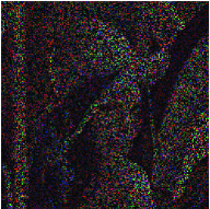
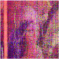
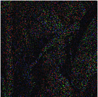
Figure 2: The comparison of different algorithms for inpainting incomplete RGB image. (From left to right) Observed images, images reconstructed by LRTI, images reconstructed by HaLRTC, images reconstructed by WTucker, images reconstructed by IRTD. Top row: $50\%$ missing. Middle row: $80\%$ missing. Bottom row: $90\%$ missing.

VI-A Synthetic and Chemometrics Data

In this subsection, we carry out experiments on synthetic and chemometrics data. Two sets of synthetic data are generated and both of them are $3$rd-order tensors of size $32\times 32\times 32$. The first tensor is generated according to the CP model which is a summation of six equally-weighted rank-one tensors, with all of the factor matrices drawn from a normal distribution. Thus the truth rank is $6$ or $(6,6,6)$ in a multilinear rank form. The other tensor is generated based on the Tucker decomposition model, with a random core tensor of size $(3,4,5)$ multiplied by random factor matrices along each mode. Clearly the groundtruth for the multilinear rank is $(3,4,5)$. Two chemometrics data sets are also considered in our simulations. One is the Amino Acid data set of size $5\times 201\times 61$ and the other is the flow injection data set of size $12\times 100\times 89$.

For each data set, we consider two cases with $50\%$ or $80\%$ entries missing in our simulations, where the missing entries are randomly selected. The observed entries are corrupted by zero mean Gaussian noise and the signal-to-noise ratio (SNR) is set to $10$dB. The tensor reconstruction performance is evaluated by the normalized mean squared error (NMSE) $\|\boldsymbol{\mathcal{X}}-\boldsymbol{\mathcal{\hat{X}}}\|_{F}/\|\boldsymbol{\mathcal{X}}\|_{F}$, where $\boldsymbol{\mathcal{X}}$ and $\boldsymbol{\mathcal{\hat{X}}}$ denote the true tensor and the estimated one, respectively. The parameter $\lambda$ for the LRTI is carefully selected as $\lambda=0.3$ for the synthetic data set generated by the Tucker model and $\lambda=0.2$ for the other data sets. The pre-defined multilinear rank for WTucker is set to be $(12,12,12)$, $(6,8,10)$, $(5,10,10)$ and $(10,10,10)$ for the CP, Tucker, Amino Acid and flow injection dataset, respectively. For our proposed method, we choose $\lambda_{1}=0.5$ for all data sets. Results are averaged over $10$ independent runs. The rank or multilinear rank is estimated as the the most frequently occurring rank or multilinear rank value. The standard deviation of the estimated rank is also reported as an indication of the stability of the inferred rank. Results are shown in Table I.

• We observe that the proposed method presents the best recovery accuracy among all algorithms and can reliably estimate the true rank.

• Compared with the CP-decomposition based method LRTI, our proposed method presents a clear performance advantage over the LRTI when synthetic data are generated according to the Tucker model and slightly outperforms the LRTI even when data are generated according to the CP model.

• Our proposed method surpasses the tensor nuclear-norm based method HaLRTC by a big margin, which corroborates our claim that the proposed group log-sum functional is more effective than the tensor nuclear-norm in approximating the multilinear rank.

• Tucker model-based methods such as HaLRTC and WTucker work well only when synthetic data are generated according to the Tucker model, while our proposed method provides decent recovery performance whether data are generated via the Tucker or CP model.

• We also observe that our proposed method has similar run times as the other three algorithms. As the number of missing entries increases, our proposed method might need a few more iterations to reach convergence, and thus the average run time increases with the number of missing entries.

VI-B Image Inpainting

TABLE II: The comparison of different algorithms for tensor completion (Image Inpainting)

	$50\%$	$80\%$	$90\%$
LRTI	$0.0023$	$0.0046$	$0.0098$
HaLRTC	$0.0019$	$0.0066$	$0.0134$
WTucker	$0.0032$	$0.0751$	$0.2187$
IRTD	$0.0015$	$0.0046$	$0.0082$

The goal of image inpainting is to complete an image with missing pixels. For a two-dimensional RGB picture, we can treat it as a three-dimensional tensor. Here we consider imputing an incomplete RGB image via respective algorithms. The benchmark Lena image is used, with $50\%$, $80\%$ and $90\%$ missing entries considered in our simulations. The recovery accuracy is evaluated by the MSE metric which is defined as $\text{MSE}=\frac{1}{M}\|\mathcal{O}^{\complement}\ast(\mathcal{X}-\hat{\mathcal{X}})\|_{F}^{2}$, where $\mathcal{X}$ and $\hat{\mathcal{X}}$ respectively denote the original normalized image and the estimated one, $\mathcal{O}^{\complement}$ denotes the complement set of the observed set, i.e. $\mathcal{O}$, and $M$ denotes the number of missing elements. For LRTI, the parameter used to control the tradeoff between the data fitting and rank is carefully selected to $5$, $3$ and $3$ for $50\%$, $80\%$ and $90\%$ missing entries, respectively. The pre-defined rank for the WTucker is set to $(100,100,3)$, $(80,80,3)$ and $(50,50,3)$ for $50\%$, $80\%$ and $90\%$ missing entries, respectively. For our proposed method, $\lambda_{1}$ is set to $3$, $0.5$ and $0.3$ for $50\%$, $80\%$ and $90\%$ missing entries, respectively. The observed and recovered images are shown in Fig.2 and MSEs of respective algorithms are shown in Table II. From Table II, we see that the proposed method renders a reliable recovery even with $90\%$ missing entries, while the other two Tuck model-based methods WTucker and HaLRTC may incur a considerable performance degradation when the missing ratio is high.

VII Conclusions

In this paper, we proposed an iterative reweighted algorithm to decompose an incomplete tensor into a concise Tucker decomposition. To automatically determine the model complexity, we introduced a new notion called order-$(N-1)$ sub-tensor and introduced a group log-sum penalty on every order-$(N-1)$ sub-tensors to achieve a structural sparse core tensor. By shrinking the zero order-$(N-1)$ sub-tensors, the core tensor becomes a smaller one and a compact Tucker decomposition can be obtained. By resorting to the majorization-minimization approach, an iterative reweight algorithm was developed. Also, the over-relaxed monotone fast iterative shrinkage-thresholding technique is adapted and embedded in the iterative reweighted process to reduce the computational complexity. The performance of the proposed method is evaluated using synthetic data and real data. Simulation results show that the proposed method offers competitive performance compared with existing methods.

References

- [1] A. Karatzoglou, X. Amatriain, L. Baltrunas, and N. Oliver, “Multiverse recommendation: n-dimensional tensor factorization for context-aware collaborative filtering,” in Proceedings of the fourth ACM conference on Recommender systems. ACM, 2010, pp. 79–86.
- [2] L. Xiong, X. Chen, T.-K. Huang, J. Schneider, and J. G. Carbonell, “Temporal collaborative filtering with Bayesian probabilistic tensor factorization,” in SDM, vol. 10. SIAM, 2010, pp. 211–222.
- [3] G. Adomavicius and A. Tuzhilin, “Context-aware recommender systems,” in Recommender systems handbook. Springer, 2011, pp. 217–253.
- [4] P. Rai, Y. Wang, and L. Carin, “Leveraging features and networks for probabilistic tensor decomposition,” in AAAI Conference on Artificial Intelligence, 2015.
- [5] I. Sutskever, J. B. Tenenbaum, and R. R. Salakhutdinov, “Modelling relational data using bayesian clustered tensor factorization,” in Advances in neural information processing systems, 2009, pp. 1821–1828.
- [6] F. Cong, Q.-H. Lin, L.-D. Kuang, X.-F. Gong, P. Astikainen, and T. Ristaniemi, “Tensor decomposition of EEG signals: A brief review,” Journal of neuroscience methods, vol. 248, pp. 59–69, 2015.
- [7] A. Cichocki, R. Zdunek, A. H. Phan, and S. I. Amari, Nonnegative matrix and tensor factorizations. John Wiley & Sons, 2009.
- [8] M. Haardt, F. Roemer, and G. D. Galdo, “Higher-order SVD-based subspace estimation to improve the parameter estimation accuracy in multidimensional harmonic retrieval problems,” IEEE Transactions on Signal Processing, vol. 56, no. 7, pp. 3198–3213, 2008.
- [9] W. Guo and W. Yu, “Variational bayesian parafac decomposition for multidimensional harmonic retrieval,” in 2011 IEEE CIE International Conference on Radar (Radar), vol. 2. IEEE, 2011, pp. 1864–1867.
- [10] E. Benetos and C. Kotropoulos, “A tensor-based approach for automatic music genre classification,” in 2008 16th European Signal Processing Conference. IEEE, 2008, pp. 1–4.
- [11] G. Zhou, A. Cichocki, Q. Zhao, and S. Xie, “Nonnegative matrix and tensor factorizations: An algorithmic perspective,” IEEE Signal Processing Magazine, vol. 31, no. 3, pp. 54–65, 2014.
- [12] Q. Li and D. Schonfeld, “Multilinear discriminant analysis for higher-order tensor data classification,” IEEE Transactions on Pattern Analysis and Machine Intelligence, vol. 36, no. 12, pp. 2524–2537, 2014.
- [13] P. Rai, Y. Wang, S. Guo, G. Chen, D. Dunson, and L. Carin, “Scalable Bayesian low-rank decomposition of incomplete multiway tensors,” in Proceedings of the 31st International Conference on Machine Learning (ICML-14), 2014, pp. 1800–1808.
- [14] L. R. Tucker, “Some mathematical notes on three-mode factor analysis,” Psychometrika, vol. 31, no. 3, pp. 279–311, 1966.
- [15] R. Bro, “PARAFAC. Tutorial and applications,” Chemometrics and intelligent laboratory systems, vol. 38, no. 2, pp. 149–171, 1997.
- [16] A. Cichocki, D. P. Mandic, H. A. Phan, C. F. Caiafa, G. Zhou, Q. Zhao, and L. D. Lathauwer, “Tensor decompositions for signal processing applications: From two-way to multiway component analysis,” IEEE Signal Processing Magazine, vol. 32, no. 2, pp. 145–163, 2015.
- [17] J. Liu, P. Musialski, P. Wonka, and J. Ye, “Tensor completion for estimating missing values in visual data,” in IEEE 12th International Conference on Computer Vision. IEEE, 2009, pp. 2114–2121.
- [18] J. A. G. Mateos and G. B. Giannakis, “Rank regularization and bayesian inference for tensor completion and extrapolation,” IEEE Transactions on Signal Processing, no. 22, pp. 5689–5703, Nov. 2013.
- [19] M. Mardani, G. Mateos, and G. B. Giannakis, “Subspace learning and imputation for streaming big data matrices and tensors,” IEEE Transactions on Signal Processing, vol. 63, no. 10, pp. 2663–2677, 2015.
- [20] E. Acar, D. M. Dunlavy, T. G. Kolda, and M. Mørup, “Scalable tensor factorizations for incomplete data,” Chemometrics and Intelligent Laboratory Systems, vol. 106, no. 1, pp. 41–56, 2011.
- [21] Y.-L. Chen, C.-T. Hsu, and H.-Y. M. Liao, “Simultaneous tensor decomposition and completion using factor priors,” IEEE Transactions on Pattern Analysis and Machine Intelligence, vol. 36, no. 3, pp. 577–591, 2014.
- [22] M. F. A. Jukić, “Tucker factorization with missing data with application to low-n-rank tensor completion,” Multidimensional Systems and Signal Processing, vol. 26, pp. 677–692, 2015.
- [23] J. Liu, P. Musialski, P. Wonka, and J. Ye, “Tensor completion for estimating missing values in visual data,” IEEE Transactions on Pattern Analysis and Machine Intelligence, vol. 35, no. 1, pp. 208–220, Jan. 2013.
- [24] Y. Liu, F. Shang, W. Fan, J. Cheng, and H. Cheng, “Generalized higher-order orthogonal iteration for tensor decomposition and completion,” in Advances in Neural Information Processing Systems, 2014, pp. 1763–1771.
- [25] A. Narita, K. Hayashi, R. Tomioka, and H. Kashima, “Tensor factorization using auxiliary information,” Data Mining and Knowledge Discovery, vol. 25, no. 2, pp. 298–324, 2012.
- [26] Q. Zhao, L. Zhang, and A. Cichocki, “Bayesian CP factorization of incomplete tensors with automatic rank determination,” IEEE Transactions on Pattern Analysis and Machine Intelligence, no. 1, pp. 1–1, 2015.
- [27] Z. Xu, F. Yan, and Y. Qi, “Bayesian nonparametric models for multiway data analysis,” IEEE Transactions on Pattern Analysis and Machine Intelligence, vol. 37, no. 2, pp. 475–487, Feb. 2015.
- [28] L. D. Lathauwer, B. D. Moor, and J. Vandewalle, “On the best rank-1 and rank- approximation of higher-order tensors,” SIAM Journal on Matrix Analysis and Applications, vol. 21, no. 4, pp. 1324–1342, 2000.
- [29] J. Håstad, “Tensor rank is NP-complete,” Journal of Algorithms, vol. 11, no. 4, pp. 644–654, 1990.
- [30] Kruskal and J. B, “Rank, decomposition, and uniqueness for 3-way and n-way arrays,” Multiway data analysis, vol. 33, pp. 7–18, 1989.
- [31] T. G. Kolda and B. W. Bader, “Tensor decompositions and applications,” SIAM review, vol. 51, no. 3, pp. 455–500, 2009.
- [32] S. Gandy, B. Recht, and I. Yamada, “Tensor completion and low-n-rank tensor recovery via convex optimization,” Inverse Problems, vol. 27, no. 2, p. 025010, 2011.
- [33] H. Tan, B. Cheng, W. Wang, Y.-J. Zhang, and B. Ran, “Tensor completion via a multi-linear low-n-rank factorization model,” Neurocomputing, vol. 133, pp. 161–169, 2014.
- [34] M. Yamagishi and I. Yamada, “Over-relaxation of the fast iterative shrinkage-thresholding algorithm with variable stepsize,” Inverse Problems, vol. 27, no. 10, p. 105008, 2011.
- [35] E. J. Candés, M. B. Wakin, and S. P. Boyd, “Enhancing sparsity by reweighted minimization,” Journal of Fourier analysis and applications, vol. 14, pp. 877–905, 2008.
- [36] R. Chartrand and W. Yin, “Iteratively reweighted algorithms for compressive sensing,” in IEEE international conference on acoustics, speech and signal processing, 2008. ICASSP 2008. IEEE, 2008, pp. 3869–3872.
- [37] D. Wipf and S. Nagarajan, “Iterative reweighted and methods for finding sparse solutions,” IEEE Journal of Selected Topics in Signal Processing, vol. 4, no. 2, pp. 317–329, 2010.
- [38] Y. Shen, J. Fang, and H. Li, “Exact reconstruction analysis of log-sum minimization for compressed sensing,” IEEE Signal Processing Letters, vol. 20, no. 12, pp. 1223–1226, 2013.
- [39] R. Tibshirani, “Regression shrinkage and selection via the lasso,” Journal of the Royal Statistical Society: Series B (Methodological), pp. 267–288, 1996.
- [40] M. Yuan and Y. Lin, “Model selection and estimation in regression with grouped variables,” Journal of the Royal Statistical Society: Series B (Statistical Methodology), vol. 68, no. 1, pp. 49–67, 2006.
- [41] D. R. Hunter and K. Lange, “A tutorial on MM algorithms,” The American Statistician, vol. 58, no. 1, pp. 30–37, 2004.
- [42] A. Beck and M. Teboulle, “A fast iterative shrinkage-thresholding algorithm for linear inverse problems,” SIAM journal on imaging sciences, vol. 2, no. 1, pp. 183–202, 2009.
- [43] L. D. Lathauwer, B. D. Moor, and J. Vandewalle, “A multilinear singular value decomposition,” SIAM journal on Matrix Analysis and Applications, vol. 21, no. 4, pp. 1253–1278, 2000.