Separation Surfaces in the Spectral TV Domain for Texture Decomposition

Abstract

In this paper we introduce a novel notion of separation surfaces for image decomposition. A surface is embedded in the spectral total-variation (TV) three dimensional domain and encodes a spatially-varying separation scale. The method allows good separation of textures with gradually varying pattern-size, pattern-contrast or illumination. The recently proposed total variation spectral framework is used to decompose the image into a continuum of textural scales. A desired texture, within a scale range, is found by fitting a surface to the local maximal responses in the spectral domain. A band above and below the surface, referred to as the Texture Stratum, defines for each pixel the adaptive scale-range of the texture. Based on the decomposition an application is proposed which can attenuate or enhance textures in the image in a very natural and visually convincing manner.

I Introduction

Decomposing an image into meaningful components is an important and challenging inverse problem in image processing. The general concept of structure-texture decomposition is that an image can be regarded as composed of a structural part, corresponding to the main large objects in the image, and a textural part, containing fine details, usually with some periodicity and oscillatory nature. Image decomposition is a preprocessing stage, which can be essential for many image processing and computer vision tasks such as segmentation [10], content based image retrieval [32] , feature extraction and classification [14] and restoration and analysis of ancient documents [12]. We first briefly recall the main approaches related to image decomposition (focusing on variational methods).

I-A Structure-texture and Multiscale Decomposition

$\bf u+v$ Model. An image $f$ can be decomposed as $f=u+v$, where $u$ represents image cartoon or geometric (piecewise-smooth) component and $v$ represents the oscillatory or textured component of $f$. This motivated [25] to suggest the $TV-G$ variational model where the minimization yields $u$ with a low total-variation energy and $v$ with a low integral norm, referred to as a $G$-norm, which favors oscillatory signals. Suggestions to implement Meyer’s model were given in [36, 3]. Many extensions and variations to the model with alternative norms adapted for textures were proposed, such as [29, 5, 24, 28, 15]. The use of nonconvex regularizers was recently proposed in [2]. Employing sparse representation methods for decomposition was first suggested in [33]. Two simplistic ways of revealing the textural parts in images are still used for some computer vision tasks. The most basic one is linear - using a smoothing kernel, such as a Gaussian, and subtracting the smoothed image from the input image. Naturally edges and textures are mixed. A somewhat more reliable method is to apply edge-preserving denoising, such as bilateral filtering [35], and subtract the result from the input image.

$\bf u+v+w$ Model. In [4] a model decomposing an image into structure $u$, texture $v$, and noise $w$ was proposed using dual norms (negative Sobolev and Besov norms) for the texture and noise parts. An analysis of the three-part decomposition can be seen in [20] and a recent approach using non-linear PDE’s for structure-texture-edge decomposition is described in [26].

Multiscale Model. It was realized quite early on that several textures of different scales can appear in an image and should be decomposed separately. Multiscale decomposition using several $TV-L^{2}$ (ROF [30]) decompositions, was first suggested in [34]. Some features interpreted as “texture” in a given scale can be interpreted as “structure” at a finer scale. As conventional ROF was used the separation was not optimal, mixing some structure in the texture. Gilles [19] combined Meyer’s decomposition model [25] with a Littlewood-Paley filter, to extract a certain class of textures in an image. While this works well for synthetic images, it is not ideal for some real world images. Zhang et al. [37] proposed a new framework called Rolling Guidance filter. This technique consists of an iterated improved variant of the bilateral filter which is controlled by a larger support linear smoothing kernel. High quality results were shown in [37]. We will compare our work also to this state-of-the-art technique and show its limitations, especially when there are gradual changes in pattern size or contrast.

Continuous Model. The spectral TV decomposition, explained in details below, can be seen as a generalization to the continuum of multiscale decomposition, with infinitesimal scale precision which can be related to the eigenvalue of the nonlinear eigenvalue problem induced by the regularizer (see details hereafter). In this case the input image is an integral over all scales. In practice the scale (time) step is finite and a summation of quantized scales is performed.

I-B Contribution and paper outline

In this paper we present two essential contributions. A new approach of scale-separation is introduced which is based on the TV transform [18]. Using a geological analogy, the texture is encoded by a stratum, with a surface as center-line, in the 3D spectral TV domain, see visualization in Fig. 1. It is well adapted to the image and can cope with gradually changing textures with respect to many parameters such as size, contrast and illumination. Having defined a general desired scale-range, the method is automatic. A second contribution is a texture processing approach which can enhance or attenuate textures in an easy manner with very vivid and natural looking results.

The outline of the paper is as follows: in Section II we describe the convex nonlinear eigenvalue problem and the spectral TV approach. Section III presents multiscale decomposition and orientation analysis based on spectral TV. This part was first presented in a conference [21]. We then proceed to the main contribution of the paper, Section IV, where a surface-based decomposition is introduced. In Section V a texture processing application is proposed, illustrated by natural color image examples.

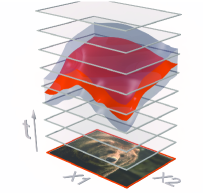
(a) Separation surface and stratum visualization

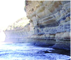
(b) Natural rock strata

Figure 1: Geological analogy of the texture encoded as a stratum in the spectral TV domain.

II Preliminaries

In this section we summarize the essential theory concerning non-linear eigenfunctions induced by convex functionals, the spectral TV framework and Gabor filters (used as scale-orientation descriptors).

II-A Nonlinear Eigenfunctions

Classical linear eigenfunction analysis has shown to provide many state-of-the-art algorithms in signal processing, computer vision and machine-learning. Some examples are segmentation [31], clustering [27], subspace clustering [23] and dimensionality reduction [6]. Eigenfunctions of an operator can be viewed as the operator’s inherent atoms with an intrinsic scale represented by the respective eigenvalue. Recent studies [7, 18] indicate that a generalized theory can be developed for the convex nonlinear case.

Nonlinear eigenfunctions induced by a convex functional emerge by the following nonlinear eigenvalue problem:

$$\lambda u\in\partial J(u),$$ (1)

where $J(u)$ is a convex functional and $\partial J(u)$ is its subdifferential. A function $u$ admitting Eq. (1) is referred to as an eigenfunction with a corresponding eigenvalue $\lambda$. We can briefly study the linear case, to get some intuition.

A Linear Example

Let us examine the functional

$$J(u)=\frac{1}{2}\int_{\Omega}|\nabla u(x)|^{2}dx,$$

where $\nabla$ is the gradient. The convex functional induces an operator through its subgradient. Here the subgradient (in this case single valued) is $p(u)=-\Delta u$ ($\Delta$ denotes the Laplacian). The corresponding eigenvalue problem is

$$-\Delta u=\lambda u.$$

In the one-dimensional case, with appropriate boundary conditions, functions of the form $u=\sin(\omega x)$ are eigenfunctions with corresponding eigenvalues $\lambda=\omega^{2}$.

Thus Fourier frequencies naturally emerge as solving an eigenvalue problem related to a quadratic smoothing convex functional.

In [17, 18] an image decomposition and filtering framework was suggested. It presents a notion of generalized nonlinear eigenfunctions which are used to define forward and inverse TV transforms. This can be used to decompose the image into well defined scales and allows a new variety of filtering methods.

II-B Spectral TV

In [18] a non-conventional way of defining a transform through a partial-differential-equation (PDE) is suggested, based on the total-variation (TV) functional:

$$J(u)=\int_{\Omega}|Du|,$$ (2)

where $Du$ denotes the distributional gradient of $u$. The corresponding gradient descent of the functional, known as total-variation flow [1], is formally written as:

$$\begin{array}[]{ll}\frac{\partial u}{\partial t}=\operatorname{div}\left(\frac{Du}{|Du|}\right),&\textrm{in }(0,\infty)\times\Omega\\ \frac{\partial u}{\partial n}=0,&\textrm{on }(0,\infty)\times\partial\Omega\\ u(0;x)=f(x),&\textrm{in }x\in\Omega,\end{array}$$ (3)

where $\Omega$ is the image domain (a bounded set in ${\rm I\kern-1.79993ptR}^{N}$ with Lipschitz continuous boundary $\partial\Omega$). The TV transform is defined by:

$$\phi(t;x)=u_{tt}(t;x)t,$$ (4)

where $u_{tt}$ is the second time derivative of the solution $u(t;x)$ of (3). The inverse transform is:

$$f(x)=\int_{0}^{\infty}\phi(t;x)dt+\bar{f},$$ (5)

where $\bar{f}=\frac{1}{\Omega}\int_{\Omega}f(x)dx$ is the mean value of the initial condition. Filtering is performed using a transfer function $H(t)\in{\rm I\kern-1.79993ptR}$:

$$f_{H}(x):=\int_{0}^{\infty}\phi(t;x)H(t)dt+\bar{f}.$$ (6)

The spectrum $S^{f}(t)$ of the input signal $f(x)$ corresponds to the $L^{1}$ amplitude of each scale:

$$S^{f}(t)=\|\phi(t;x)\|_{L^{1}}=\int_{\Omega}|\phi(t;x)|dx.$$ (7)

Two significant results were shown in [18] for this transform:

• Eigenfunctions as Atoms: Let $f(x)$ be a function which admits the nonlinear eigenvalue problem (1), ($f=u$), for the TV functional. Then the transform yields a measure (single impulse), multiplied by $f(x)$, at time $t=1/\lambda$ and is zero for all other $t$: $\phi(t;x)=\delta(t-1/\lambda)f(x)$, where $\delta(\cdot)$ is the Dirac delta function.

• Relations to TV-flow: The TV flow solution $u(t)$ is given by:

  $$u(t)=\int_{0}^{\infty}H^{t}(\tau)\phi(\tau;x)d\tau+\bar{f};\,\,\,$$ (8)

  $$H^{t}(\tau)=\left\{\begin{array}[]{ll}0,&0\leq\tau<t\\ \frac{\tau-t}{\tau},&t\leq\tau<\infty\end{array}\right..$$

The first result relates to nonlinear spectral theory, which has attracted increasing interest lately, see e.g. [7, 16] and [8] in the segmentation and learning context.

The second result shows that the framework is a generalization of standard TV filters and that many other filters related to the functional can be designed.

An example of different spectral components and of spectral image filtering can be seen in Fig. 2. A zebra image is shown with its spectrum in different colors to demonstrate the integration intervals of the $\phi$’s, using (6) with $H=1$ in the desired interval and 0 otherwise, appearing respectively in the filtered images. The contrast is enhanced for better visualization.

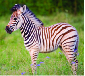
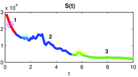
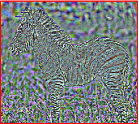
(a) High-pass

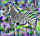
(b) Band-pass

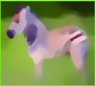
(c) Low-pass

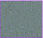
(d) $t=0.4$

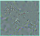
(e) $t=1.6$

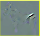
(f) $t=5.8$

Figure 2: Zebra image (top left), TV spectrum of the image with separated textures marked in different colors (top right), and spectral decomposition of the zebra image to textures, displaying integration over time (middle) and certain $\phi$’s (bottom).

II-C Gabor Filters

A Gabor filter bank is a set of regularly spaced filters that roughly mimic the behavior of the human visual system (HVS) for texture detection. According to this model, the HVS perceives the image through a set of filtered images, so that each image contains some unique visual information over a narrow range of orientation channel. In that manner, Gabor filtering has been shown to be a good fitting to this model, providing optimal localization of image details in a joint spatial and frequency domain [22, 13]. The Gabor wavelet definition is

$$g(x,y)=\frac{1}{2\pi\sigma_{x}\sigma_{y}}exp[-\frac{1}{2}(\frac{\tilde{x}^{2}}{{\sigma_{x}}^{2}}+\frac{\tilde{y}^{2}}{{\sigma_{y}}^{2}})+2\pi jW\tilde{x}]$$ (9)

$$\tilde{x}={x\cos(\frac{\mu\pi}{M})+y\sin(\frac{\mu\pi}{M})},\tilde{y}={-x\sin(\frac{\mu\pi}{M})+y\cos(\frac{\mu\pi}{M})}$$ (10)

$\mu$ controls the orientation of the filters, with M being the total number of different orientations and $W$ scales the center of the filter in the frequency domain.

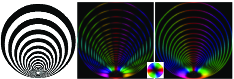
Figure 3: Concentric circles image (left), orientation map of 8 Gabor filters response (middle) and orientation map of 30 Gabor filters response (right).

III Multiscale Decomposition Using Spectral TV

In this section we show how one can use spectral TV for multiscale decomposition and multiscale orientation analysis. This part was first presented by the authors in a conference [21]. In this work we extended the common structure and texture decomposition to multi-scale texture separation in order to get all textures, the coarse and fine-scaled. The orientation of the different texture layers was separately characterized using the Gabor filters bank, generating the scale-orientation descriptor. Precise orientation mapping can be useful for analysis and inner texture actions and synthesis of image with complex textures content.

III-A A Necessary Condition for Perfect Separability

In [9] an orthogonality relation between $\phi$, Eq. (4), and $u$ is established:

$$\langle u(t),\phi(t)\rangle=0,\forall t\in(0,\infty),$$ (11)

where $\langle\cdot,\cdot\rangle$ denotes the $L^{2}$ inner product over the domain $\Omega$. Using the above relation and the one given in (8) a necessary condition for perfect separability of eigenfunctions can be shown:

Proposition 1.

Let $f_{1}(x)$, $f_{2}(x)$ admit the eigenvalue problem (1), with $J$ the TV functional (2), and $\lambda_{1}$, $\lambda_{2}$ the corresponding eigenvalues ($\lambda_{1}>\lambda_{2}$). Then for $f=f_{1}+f_{2}$ a necessary condition to have

$$\phi(t)=\delta(t-\frac{1}{\lambda_{1}})f_{1}(x)+\delta(t-\frac{1}{\lambda_{2}})f_{2}(x),$$ (12)

is

$$\langle f_{1},f_{2}\rangle=0.$$

Proof.

Let us assume Eq. (12) holds and $\langle f_{2}(x),f_{1}(x)\rangle\neq 0$. We express $u(t_{1})$ using (8), with $t_{1}:=\frac{1}{\lambda_{1}}$ (note that $H^{t_{1}}(t_{1})=0$):

$$u(t_{1})=\int_{t_{1}}^{\infty}H^{t_{1}}(\tau)\phi(\tau;x)d\tau=H^{t_{1}}(t_{2})f_{2}(x).$$

From Eq. (11) we have

$$\langle u(t_{1}),\phi(t_{1})\rangle=0,$$

and therefore

$$H^{t_{1}}(t_{2})\delta(t=0)\langle f_{2}(x),f_{1}(x)\rangle=0,$$

which contradicts our assumption. ∎

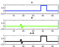
(a) Signals

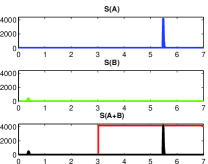
(b) TV spectrums

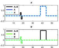
(c) Spec TV (proposed) result

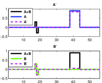
(d) TV result

Figure 4: Separating 1D orthogonal signals.

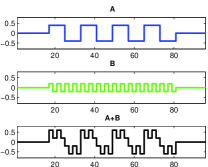
(a) Signals

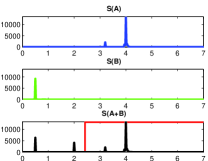
(b) TV spectrums

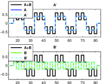
(c) Spec TV (proposed) result

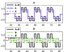
(d) TV result

Figure 5: Separating 1D oscillating uncorrelated signals

Note that in the case of perfect separability, Eq. (12), simple spectral filtering (6) with $H(t)=1$ for $t<t_{c}$ and $0$ otherwise, where $t_{c}\in(1/\lambda_{1},1/\lambda_{2})$, can perfectly separate $f_{1}$ and $f_{2}$. Examples demonstrating the signals’ separability in 1D are shown in Figs. 4-5. Separation of the larger scale signal is performed using (6) with $H(t)$ a step signal ($\{0,1\}$ values) as superimposed in red on the combined spectrum plot (bottom of Figures 4-5 (b)). In Fig. 4 two well-separated orthogonal signals are shown, their spectrum, Eq. (7), has one peak for each signal, and the combined spectrum $S^{(A+B)}(t)$ is the sum $S^{A}(t)+S^{B}(t)$. Decomposition using spectral TV yields a perfect separation. We can see also the optimal possible result of standard TV regularization for comparison. Note that the standard TV does not yield perfect separation and the decomposition mixes both signals. In Fig. 5, two orthogonal oscillating signals are combined. Their combined spectrum slightly changes, compared to the original isolated signals, as a result of the overlap. However they can still be perfectly separated using spectral TV, while the standard TV has significant artifacts and the signals are not well separated. We use the projection algorithm of Chambolle [11] to implement the TV-flow time steps [18]. For more details, see http://guygilboa.eew.technion.ac.il/code/.

III-B Image Decomposition

Decomposition using spectral TV was applied to textured images. The decomposition can be done to as many different layers as required, limited numerically only by the chosen time step (the theoretical formulation is continuous in time). An example of such image decomposition can be seen in Fig. 6. A game board image is shown with its spectrum in different colors to demonstrate the separation points of the decomposition (or integration intervals of the $\phi$’s, using (6) with $H=1$ in the desired interval and 0 otherwise) appearing respectively in Fig. 7: the wood pattern , the game board lines and the structure with the round game pieces. In this example, the separation points of the decomposition were manually chosen. However, in [5] it was done automatically for structure-texture decomposition using correlation between the texture and the residual structure in each level. In the next section of this work we explore the automatic texture separation.

III-C Scale-Orientation Descriptor

After decomposing the image we generate the scale-orientation descriptor (SOD) for each texture level by fully mapping its orientation, creating a multi-valued orientation descriptor for each pixel. This was achieved using the Gabor filter bank. The Gabor filter response was calculated in 30 orientations ($M=30,\mu=0,1,...,30$), spanning 180°  and 4 spatial frequencies for finer and coarser scales. In Fig. 3 presented a concentric circles image (left) and the colored orientation map of 8 (middle) and 30 (right) Gabor filters response. In each scale, the orientation giving the maximum response was selected, and the maximum of the 4 scales was taken to describe the orientation of each pixel.

An example of such scale-orientation descriptor can be seen in Fig. 7. In this figure, decomposition of the game board image (Fig. 6) to three scales is shown, together with the corresponding orientation mapping images. We can observe the great separation of the different layers as seen in the colored orientation figures as processed from the Gabor filters response. The orientation in each pixel is taken from the Gabor scale which gave the strongest response, usually corresponding to the texture coarseness. The result of Gilles decomposition [19] for this image are on Fig. 8, as can be seen, the textures nicely appear there in different scales but the different textures are not separated.

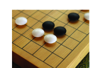
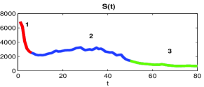
Figure 6: Game board image (left) and TV spectrum of the image with separated textures marked in different colors (right)

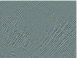
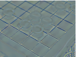
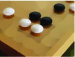
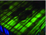
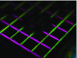
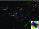
Figure 7: SOD of Game board image (Fig. 6). Our multi scale decomposition of the image (top) and the corresponding orientation maps (bottom). (The contrast is enhanced for better visualization.)

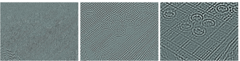
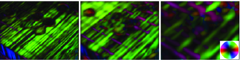
Figure 8: Compared method [19] decomposition result for game board image to 3 scales (top) and Gabor orientation visualization (bottom)

IV Separation Surface

We now present the novel notion of the separation surface. The texture decomposition so far was done assuming that our texture is homogeneous and can be separated at a certain configuration which fits the whole image. However, that is not the situation in many natural images, in which, due to changing texture, lighting conditions, or perspective, the desired texture can not be decomposed in the same configuration for the entire image. For that purpose we introduce the separation surface. It is a decomposition configuration, changing in a continuous manner in the image according to the texture. We first characterize the different textures in the image to find the spectral time band of the desired texture. We then determine the exact spectral layer ($\phi$) for each pixel in a global manner to ensure smoothness of the extracted texture, under the assumption of texture being smooth and continuous. We define a band surrounding the surface to capture the entire features of the desired texture. We call it stratum. In geology and related fields, a stratum is a layer of sedimentary rock or soil with internally consistent characteristics that distinguish it from other layers. Similarly, in our case, the stratum defines a certain texture, distinguished from other by its features. It consists of the spectral layers forming the desired texture for each pixel. A figure simulating the separation surface can be seen in Fig. 1, as well as an image of natural rock stratum.

IV-A Analytic Example

We begin by examining an analytic example to understand the surface fitting process. It is well established that disks are elementary structures for the TV functional. They satisfy the eigenvalue problem (1) which implies their shape stays the same during a TV gradient descent evolution (TV-flow [1]). Moreover, the eigenvalue of a disc of radius $r$ and height $h$ is inverse proportional to those measures [25, 1]:

$$\lambda\propto\frac{1}{hr},$$ (13)

where in the spectral TV domain we have the discs appear at scale $t=\frac{1}{\lambda}\propto hr$. We would like to analyse the image in Fig. 9, containing synthetic discs in varying size and contrast. In order to do so, we will recall two properties of spectral TV [18]:
Contrast change.

$$f(x)\to af(x),\,\,\phi(t,x)\to\phi(t/a,x),\,\,S(t)\to S(t/a).$$

Spatial scaling (2D).

$$f(x)\to f(ax),\,\,\phi(t,x)\to a\phi(at,ax),\,\,S(t)\to a^{-1}S(at).$$

For example, for an image which is half the size of the original image, we have a = 2.

The effect of the contrast change in our example is that the darker the discs (lower contrast), their scale is lower. The effect of the scale change is that the smaller the discs, their scale is lower. In this example one can see how the scale and the maximal $\phi$ value gradually changes with size and contrast. Following this analytic example we can understand the spectral TV behaviour of different images and textures.

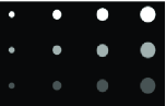
(a) Input image

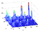
(b) Max Phi Value

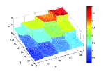
(c) Max. Time

Figure 9: Input image of discs varying in size and contrast (a), the maximal $\phi$ value (b) and the evolution time (c)

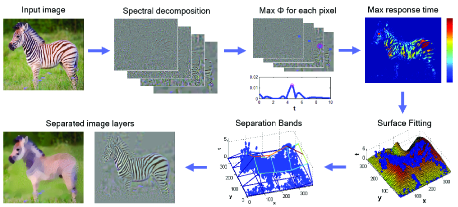
Figure 10: Algorithm flow of the separation surface

IV-B Algorithm

We present a separation surface algorithm using the TV spectral framework. The idea is that natural textures are not homogeneously distributed in scale and space, instead they continuously vary in the image. Under that assumption we suggest a decomposition configuration, changing in a continuous manner in the image according to the texture. The spectral framework allows a straightforward way to achieve such complex decomposition. The general approach can be described as follows:

1. Compute the spectral components $\phi(t)$ and the spectrum $S(t)$.

2. Manually or automatically, analyze the spectrum and choose the spectral components $\phi(t)$, $t_{1}\leq t\leq t_{2}$, among which the desired texture stretches.

3. Create a salient time map $T(x)$: for each pixel $x$, take $t$ which maximizes $\phi(t,x)$ within the range $t\in[t_{1},t_{2}]$.

4. Filter $T(x)$ to enable good surface fitting.

5. Fit a surface using regression to the corresponding filtered time mapping.

6. Calculate the bands below and above the surface to get the integration times of the desired texture in each pixel.

7. Reconstruct the desired texture layer by integrating over the texture stratum, using:

   $$f_{H}(x)=\int_{0}^{\infty}{}H(t;x)\phi(t;x)dt,\\$$ (14)

   $$H(t;x)=\left\{\begin{matrix}1&(t;x)\in stratum\\ 0&else\end{matrix}\right.$$

Notes

• We take the maximum $\phi$ among the selected spectral components under the assumption that in the scale range of the desired texture, it is dominant and therefore its response on those spectral components is high, and at most times, higher than the other patterns in those scales.

• Filtering of the maximal $\phi$ can include omitting values on image boundaries, taking only $\phi$ values at limited percentiles (we used percentile range of 85-95) etc..

• The band width is set according to the scale of the surface at each image location. The band is wider at higher spectral scales, due to smear effect with time (Fig. 11(c)).

Figure 10 illustrates the proposed algorithm of the separation surface. Zebra image was taken, to extract the stripes texture. It can be vividly seen that for coarse stripes texture, later times are taken, and larger separation band accordingly. The output is the two separated image layers, of the zebra stripes and the image residual. One can see that all the stripes are extracted, coarse and fine, with high and low contrast, while successfully preserving the edges in the residual image.

IV-C First Order Surface Examples

Favourably, we work with first order surfaces, since it allows us to better regulate the data and dismiss outliers, and due to its robustness. Later we show that it can be generalized to surfaces of higher order. Let us examine a synthetic example. A texture was taken of the Brodatz texture database, and was added a pattern of circles horizontally varying in contrast, Fig. 11. In this example, we can see in the separation band image that the base texture and the circles are not separated in scale, and the fitted separation plane and the band taken, manage to capture the entire circles features while including just a bit of the base texture, and only on the left of the image, where the contrast of the circles is low and their spectral scale is similar to that of the base texture. Our separation result is very good and highly resembles the original textures. Comparisons to TV-G and to RGF are shown where in both cases the separation is not good and residual of the textures vividly remains in both the layers. Another example is shown on Fig. 12 of street tiles, one can see the pattern is homogeneous in nature but in the image it is linearly changing due to perspective point of view. We decomposed that image using the spectral TV filtering, and took the max $\phi$ time mapping. We can see it captures the linear change in the vertical direction of the image. The upper side is far from the photographer, thus details are small and the evolution time is short. The bottom of the image is close, thus details are coarser and the resulting evolution time is longer. Taking the stratum accordingly, we capture the entire texture in one image and the structure in another image, with sharp edges, and no tiles remainder. We compared this result to the state-of-the-art RGF result [37] which suggest a multi-scale decomposition scales, we show here the 2nd and 3rd scales. In both of them, there can be seen a difference between the lower and upper sides of the image. In the 2nd scale there are many tiles edges, mostly on the lower side of the image, and in the 3rd scale, the structure edges are already smeared, especially at the upper side of the image.

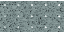
(a) Synthesized input image

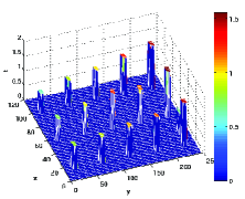
(b) Max. $\phi$ time

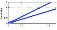
(c) Band width

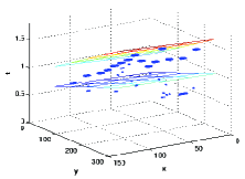
(d) Separation band

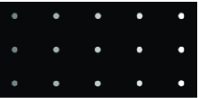
(e) Texture 1 - original

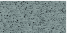
(f) Texture 2 - original

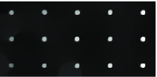
(g) Decomposed layer 1 - proposed

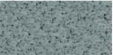
(h) Decomposed layer 2 - proposed

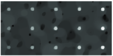
(i) TV-G, layer 1

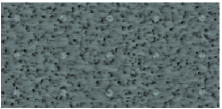
(j) TV-G, layer 2

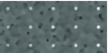
(k) RGF, layer 1

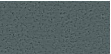
(l) RGF, layer 2

Figure 11: Separation plane of a synthetic example

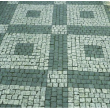
(a) Input image

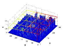
(b) Max. Phi time with separation band

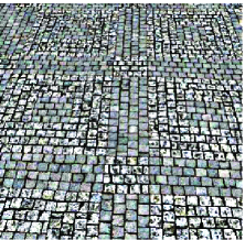
(c) Proposed texture

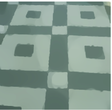
(d) Proposed structure

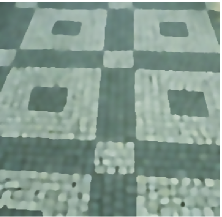
(e) RGF decomposition: scale 2

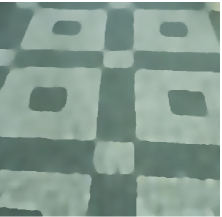
(f) RGF decomposition: scale 3

Figure 12: Multiscale separation of Street tiles image and comparison to RGF method

IV-D Generalization to Surfaces

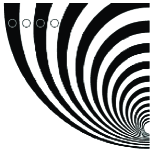
(a) Input image

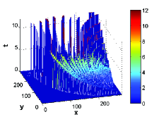
(b) Max. $\phi$ time

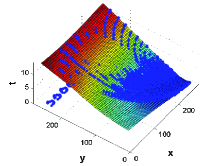
(c) Texture surface

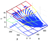
(d) Separation band

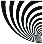
(e) Decomposed layer 1 - proposed

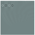
(f) Decomposed layer 2 - proposed

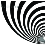
(g) $t_{s}=0.6$, layer 1

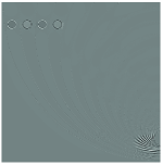
(h) $t_{s}=0.6$, layer 2

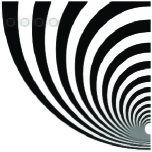
(i) TV-G, layer 1

(j) TV-G, layer 2

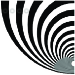
(k) RGF, layer 1

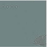
(l) RGF, layer 2

Figure 13: Decomposition of concentric circles image using a separation surface and comparison to TV-G and RGF.

We now show the general approach of separation surface or stratum extraction. We use this general approach when desired texture is more complex and does not linearly change in the image space. In this case we will perform the exact same actions to find the separation plane, but instead of fitting a plane to the texture filtered max. time data, we fit a surface. We present here a simple method for surface fitting, using local linear regression, in Fig 13. In this example, we added 4 disks to an image of concentric circles with changing radius. We can see in the separation band image that the disks and the fine scales circles are at the same spectral scale, however, their spatial location in the image is different, and so, using a separation surface, the two textures are perfectly separated. We can see a comparison to separation at a specific time (scale) for the whole image, as was done in our previous work [21]. In this case, while not all the disks features are captured in layer 2, the circles features are already contained in that layer, meaning that separating at any certain scale can not bring to a perfect separation. More comparisons are to TV-G and to the state of the art RGF [37], which both fail getting good separating result. Another example can be seen in the algorithm description (Fig. 10), where in the zebra image, the stripes were very nicely separated from its structure. The separation surface can be optimally found in different manners, according to the texture’s features. One of them is to use the Gabor filters in order to find a separation surface for textures with definite texture orientation. Another option is to use the Gaussian Mixture Model in order to differentiate textures with different distribution in space and time, and adapt the separation surface to it.

V Applications

V-A Texture Manipulation

Following an efficient texture separation, we can manipulate the different image layers in order to create sub-images, with enhanced texture or reduced texture. For example, in Fig 14 we separate the faces only, maintaining the sharp stones’ borders, and then, manipulate their level in the output image to get enhanced or depressed facial features. In Fig. 15 another texture manipulation example is shown, where the wood texture in the game board image is depressed and enhanced to a desired level. In the zebra image in Fig. 16 the stripes were extracted as depicted in Fig. 10, then by using a mask of the zebra itself, the stripes were enhanced and then inverted, so that the brown and white colors were replaced. Note that because of the stratum definition, including mostly the stripes, the other zebra features, such as nose and eyes maintained their color.

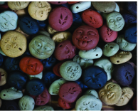
(a) Input Image

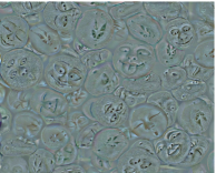
(b) Desired Texture

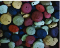
(c) Attenuated texture

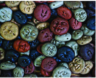
(d) Enhanced texture

Figure 14: Example of manipulation of faces’ features in the image of Faces on stones

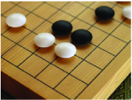
(a) Input Image

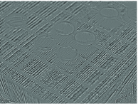
(b) Desired texture

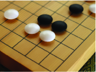
(c) Attenuated texture

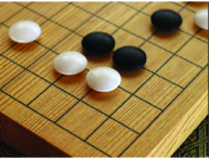
(d) Enhanced texture

Figure 15: Example of manipulation of the wood texture in the game board image

(a) Input image

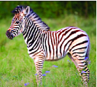
(b) Enhanced stripes

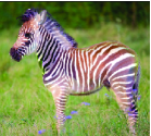
(c) Inverted stripes

Figure 16: Stripes extraction and manipulation in the Zebra image.

V-B Texture Donation

Another application is texture donation, in which a degraded image is enhanced and its fine texture is recovered by matching a prior out of a set, using our scale-orientation descriptor, to get a perfect patch match and visually good recovery of the image. In Fig. 17 we can see a hair example, on the left image a degraded hair sample is shown, in the middle is the matching hair texture donor, selected out of many hair priors. Its mirror image was taken for a texture match. On the right, the recovered hair image, composed of the degraded texture patch and decomposed fine scale texture of the donor patch. We can see the recovered patch inside the original hair image to see how natural it looks.

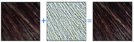
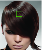
(a) Degraded

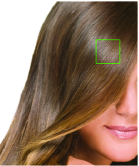
(b) Donor

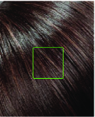
(c) Recovered

Figure 17: Hair texture donation example.

VI Conclusion

A novel concept of separation surface was introduced, depicting a stratum of a desired texture, not necessarily homogeneous in space and scale. The surface was found using regression of the maximal responses in the spectral TV domain. The surface can be fitted using methods other than maximal response, such as the Gabor filters for orientated textures, or the Gaussian mixture model for a mixture of textures with different distribution in space and scale. Image decomposition using a separation surface can be very beneficial in cases where the texture varies within the image, while preserving its characteristic. It can separate mixed textures in a highly accurate manner, compared to state-of-the-art methods. An application of texture manipulation was presented, in which the selected textures in the image can be attenuated, enhanced or even inverted, in a naturally looking formation. In a future work, we plan to examine additional methods to automatically form the surface. We would also like to broaden the use of multiscale decomposition to other applications.

Dikla Horesh received the B.Sc. degree in Biomedical engineering from the Technion, Israel, in 2006. She is currently working towards the M.Sc. degree in Electrical engineering from the Technion, Israel.

Guy Gilboa is a faculty member at the Electrical Engineering Department, Technion, Israel, since 2013.

References

- [1] F. Andreu, C. Ballester, V. Caselles, and J. M. Mazón, “Minimizing total variation flow,” Differential and Integral Equations, vol. 14, no. 3, pp. 321–360, 2001.
- [2] A. Atto and G. Mercier, “High order structural image decomposition by using non-linear and non-convex regularizing objectives,” To appear, Computer Vision and Image Understanding, 2015.
- [3] J. Aujol, G. Aubert, L. Blanc-Féraud, and A. Chambolle, “Image decomposition into a bounded variation component and an oscillating component,” JMIV, vol. 22, no. 1, 2005.
- [4] J. Aujol and A. Chambolle, “Dual norms and image decomposition models,” IJCV, vol. 63, no. 1, pp. 85–104, June 2005.
- [5] J. Aujol, G. Gilboa, T. Chan, and S. Osher, “Structure-texture image decomposition – modeling, algorithms, and parameter selection,” Int. J. Computer Vision, vol. 67, no. 1, pp. 111–136, 2006.
- [6] M. Belkin and P. Niyogi, “Laplacian eigenmaps for dimensionality reduction and data representation,” Neural computation, vol. 15, no. 6, pp. 1373–1396, 2003.
- [7] M. Benning and M. Burger, “Ground states and singular vectors of convex variational regularization methods,” Methods and Apps. of Anal., vol. 20, no. 4, pp. 295–334, 2013.
- [8] X. Bresson, X.-C. Tai, T. Chan, and A. Szlam, “Multi-class transductive learning based on relaxations of cheeger cut and mumford-shah-potts model,” Journal of mathematical imaging and vision, vol. 49, no. 1, pp. 191–201, 2014.
- [9] M. Burger, L. Eckardt, G. Gilboa, and M. Moeller, “Spectral representations of one-homogeneous functionals,” in Proc. Scale Space and Variational Methods in Computer Vision. SSVM, 2015.
- [10] W. Casaca, A. Paiva, E. Gomez-Nieto, P. Joia, and L. G. Nonato, “Spectral image segmentation using image decomposition and inner product-based metric,” Journal of mathematical imaging and vision, vol. 45, no. 3, pp. 227–238, 2013.
- [11] A. Chambolle, “An algorithm for total variation minimization and applications,” JMIV, vol. 20, pp. 89–97, 2004.
- [12] M. Coustaty, S. Dubois, M. Menard, and J.-M. Ogier, “Ancient documents denoising and decomposition using aujol and chambolle algorithm,” in Graphics Recognition. New Trends and Challenges. Springer, 2013, pp. 15–24.
- [13] J. G. Daugman, “Two-dimensional spectral analysis of cortical receptive field profiles,” Vision research, vol. 20, no. 10, pp. 847–856, 1980.
- [14] S. Dua, U. R. Acharya, P. Chowriappa, and S. V. Sree, “Wavelet-based energy features for glaucomatous image classification,” Information Technology in Biomedicine, IEEE Transactions on, vol. 16, no. 1, pp. 80–87, 2012.
- [15] V. Duval, J. Aujol, and L. Vese, “Projected gradient based color image decomposition,” in Scale Space and Variational Methods in Computer Vision. Springer, 2009, pp. 295–306.
- [16] D. Giannakis and A. Majda, “Nonlinear laplacian spectral analysis for time series with intermittency and low-frequency variability,” Proceedings of the National Academy of Sciences, vol. 109, no. 7, pp. 2222–2227, 2012.
- [17] G. Gilboa, “A spectral approach to total variation,” in A. Kuijper et al. (Eds.): SSVM 2013, ser. LNCS, vol. 7893. Springer, 2013, pp. 36–47.
- [18] ——, “A total variation spectral framework for scale and texture analysis,” SIAM J. Imaging Sciences, vol. 7, no. 4, pp. 1937–1961, 2014.
- [19] J. Gilles, “Multiscale texture separation,” Multiscale Modeling & Simulation, vol. 10, no. 4, pp. 1409–1427, 2012.
- [20] J. Gilles and Y. Meyer, “Properties of bv- g structures+ textures decomposition models. application to road detection in satellite images,” IEEE Transactions on Image Processing, vol. 19, no. 11, pp. 2793–2800, 2010.
- [21] D. Horesh and G. Gilboa, “Multiscale texture orientation analysis using spectral total-variation decomposition,” in Scale Space and Variational Methods in Computer Vision. Springer, 2015, pp. 486–497.
- [22] A. K. Jain and F. Farrokhnia, “Unsupervised texture segmentation using gabor filters,” Pattern Recognition, vol. 24, no. 12, pp. 1167–1186, 1991.
- [23] G. Liu, Z. Lin, S. Yan, J. Sun, Y. Yu, and Y. Ma, “Robust recovery of subspace structures by low-rank representation,” Pattern Analysis and Machine Intelligence, IEEE Transactions on, vol. 35, no. 1, pp. 171–184, 2013.
- [24] P. Maurel, J.-F. Aujol, and G. Peyré, “Locally parallel texture modeling,” SIAM Journal on Imaging Sciences, vol. 4, no. 1, pp. 413–447, 2011.
- [25] Y. Meyer, “Oscillating patterns in image processing and in some nonlinear evolution equations,” March 2001, the 15th Dean Jacquelines B. Lewis Memorial Lectures.
- [26] J. Moreno, V. Prasath, D. Vorotnikov, H. Proenca, and K. Palaniappan, “Adaptive diffusion constrained total variation scheme with application to cartoon+ texture+ edge image decomposition,” arXiv preprint arXiv:1505.00866, 2015.
- [27] A. Ng, M. Jordan, and Y. Weiss, “On spectral clustering: Analysis and an algorithm,” Advances in neural information processing systems, vol. 2, pp. 849–856, 2002.
- [28] M. Nikolova, “A variational approach to remove outliers and impulse noise,” JMIV, vol. 20, no. 1-2, pp. 99–120, 2004.
- [29] S. Osher, A. Sole, and L. Vese, “Image decomposition and restoration using total variation minimization and the H-1 norm,” SIAM Multiscale Modeling and Simulation, vol. 1, no. 3, pp. 349–370, 2003.
- [30] L. Rudin, S. Osher, and E. Fatemi, “Nonlinear total variation based noise removal algorithms,” Physica D, vol. 60, pp. 259–268, 1992.
- [31] J. Shi and J. Malik, “Normalized cuts and image segmentation,” IEEE Transactions on Pattern Analysis and Machine Intelligence, vol. 22, no. 8, pp. 888–905, 2000.
- [32] M. Singha and K. Hemachandran, “Content based image retrieval using color and texture,” Signal & Image Processing: An International Journal (SIPIJ), vol. 3, no. 1, pp. 39–57, 2012.
- [33] J.-L. Starck, M. Elad, and D. L. Donoho, “Image decomposition via the combination of sparse representations and a variational approach,” Image Processing, IEEE Transactions on, vol. 14, no. 10, pp. 1570–1582, 2005.
- [34] E. Tadmor, S. Nezzar, and L. Vese, “A multiscale image representation using hierarchical (BV,L2) decompositions,” SIAM Multiscale Modeling and Simulation, vol. 2, no. 4, pp. 554–579, 2004.
- [35] C. Tomasi and R. Manduchi, “Bilateral filtering for gray and color images,” in ICCV ’98, 1998, pp. 839–846.
- [36] L. Vese and S. Osher, “Modeling textures with total variation minimization and oscillating patterns in image processing,” Journal of Scientific Computing, vol. 19, pp. 553–572, 2003.
- [37] Q. Zhang, X. Shen, L. Xu, and J. Jia, “Rolling guidance filter,” in Computer Vision–ECCV 2014. Springer, 2014, pp. 815–830.