Cosmic tidal reconstruction

Abstract

The gravitational coupling of a long-wavelength tidal field with small-scale density fluctuations leads to anisotropic distortions of the locally measured small-scale matter correlation function. Since the local correlation function is known to be statistically isotropic in the absence of such tidal interactions, the tidal distortions can be used to reconstruct the long-wavelength tidal field and large-scale density field in analogy with the cosmic microwave background lensing reconstruction. In this paper we present the theoretical framework of cosmic tidal reconstruction and test the reconstruction in numerical simulations. We find that the density field on large scales can be reconstructed with good accuracy and the cross-correlation coefficient between the reconstructed density field and the original density field is greater than 0.9 on large scales ($k\lesssim 0.1\ h/\mathrm{Mpc}$), with the filter scale $\sim 1.25\ \mathrm{Mpc}/h$. This is useful in the 21cm intensity mapping survey, where the long-wavelength radial modes are lost due to a foreground subtraction process.

I Introduction

The large-scale structure contains a wealth of information about our Universe. The cosmic acceleration, neutrino masses, early Universe models and other properties of the Universe can be inferred with current or upcoming surveys. The initially linear and Gaussian density perturbations grow due to gravitational interaction; the nonlinearities develop and induce the couplings between different modes. This leads to striking non-Gaussian features in the large-scale structure of the Universe, limiting the cosmological information that can be extracted from galaxy surveys. However, such correlations between the different perturbation modes on different scales imply that we could infer the large-scale density field by observing small-scale density fluctuations.

The basic idea is that the evolution of small-scale density perturbations $\delta(\bm{k}_{S})$ is modulated by long-wavelength perturbations $\Phi_{L}$, causing both isotropic and anisotropic distortions of the local small-scale power spectrum Schmidt et al. (2014). The isotropic distortion, which only depends on the magnitude of the wave vector $\bm{k}_{S}$, is mainly due to the change in the background density from the long-wavelength density perturbation $\nabla^{2}\Phi_{L}\propto\delta_{L}$, where $\Phi_{L}$ denotes the long-wavelength gravitational potential. The anisotropic distortion, which also depends on the direction of $\bm{k}_{S}$, is induced by the long-wavelength tidal field $t_{ij}=\Phi_{L,ij}-\delta_{ij}\nabla^{2}\Phi_{L}/3$, where $\Phi_{L,ij}\equiv\partial^{2}\Phi_{L}/\partial x^{i}\partial x^{j}$. Using the isotropic modulation on the small-scale power spectrum to reconstruct the large-scale density field has been studied in Ref. Li et al. (2014). However, the anisotropic distortions are more robust since many other processes can lead to isotropic distortions in the local small-scale power spectrum. By applying quadratic estimators, which quantify the local anisotropy of small-scale density statistics, the long-wavelength tidal field can be reconstructed accurately Pen et al. (2012). The reconstruction of the long-wavelength tidal field from the local small-scale power spectrum is similar to the reconstruction of shear fields in gravitational lensing Lu and Pen (2008); Lu et al. (2010).

In this paper, we investigate the anisotropic method in detail. The evolution of small-scale density fluctuations in the presence of the long-wavelength tidal field $t_{ij}$ has been studied extensively in Ref. Schmidt et al. (2014). The tidal distortion of the local small-scale power spectrum is given by

$$P(\bm{k}_{S},\tau)|_{t_{ij}}=P_{1s}(k_{S},\tau)+\hat{k}_{S}^{i}\hat{k}_{S}^{j}t_{ij}^{(0)}P_{1s}(k_{S},\tau)f(k_{S},k_{L},\tau),$$ (1)

where $\hat{\bm{k}}$ denotes the unit vector in the direction of $\bm{k}$, $P_{1s}(k_{S},\tau)$ is the isotropic linear power spectrum, $f(k_{S},k_{L},\tau)$ describes the coupling of the long-wavelength tidal field to the small-scale density fluctuations and superscript $(0)$ denotes some “initial” time. The traceless $3\times 3$ tensor $t_{ij}$ can be decomposed into five independently observable components

$$t_{ij}=\left(\begin{array}[]{ccc}\gamma_{1}-\gamma_{z}&\gamma_{2}&\gamma_{x}\\ \gamma_{2}&-\gamma_{1}-\gamma_{z}&\gamma_{y}\\ \gamma_{x}&\gamma_{y}&2\gamma_{z}\end{array}\right),$$ (5)

where $\gamma_{1}=(\Phi_{L,11}-\Phi_{L,22})/2$ and $\gamma_{2}=\Phi_{L,12}$ are the only two tidal shear fields that do not involve $i=3$ (see Sec. III.1 for more details). In this paper we take the third axis to be parallel with the line of sight $(x_{\parallel}=x^{3})$ and the first and second axes to lie in the tangential plane perpendicular to the line of sight $[\bm{x}_{\perp}=(x^{1},x^{2})]$. The anisotropic distortion can also be decomposed into five orthogonal quadrupolar distortions as in weak lensing. While $t_{ij}$ in principle has five independently observable components, in this paper we shall focus on the two transverse shear terms, $(\hat{k}_{1}^{2}-\hat{k}_{2}^{2})\gamma_{1}^{(0)}P_{1s}f$ and $2\hat{k}_{1}\hat{k}_{2}\gamma_{2}^{(0)}P_{1s}f$, which describe quadrupolar distortions in the tangential plane perpendicular to the line of sight. The quadrupolar distortions containing $i=3$ will be affected by peculiar velocities and require additional treatments beyond the scope of this paper. These two tidal shear fields $\gamma_{1}$ and $\gamma_{2}$ can be converted into the two-dimensional (2D) convergence field, $\kappa_{\mathrm{2D}}\equiv(\Phi_{L,11}+\Phi_{L,22})/2$, using the relation

$$\kappa_{\mathrm{2D},11}+\kappa_{\mathrm{2D},22}=\gamma_{1,11}-\gamma_{1,22}+2\gamma_{2,12}.$$ (6)

We can obtain the three-dimensional (3D) convergence field $\kappa_{\mathrm{3D}}\equiv\nabla^{2}\Phi_{L}/3$ from the 2D convergence by

$$\kappa_{\mathrm{3D,11}}+\kappa_{\mathrm{3D,22}}=\frac{2}{3}\nabla^{2}\kappa_{\mathrm{2D}}.$$ (7)

The large-scale density field $\delta_{L}$ is then given by the 3D convergence field through the Poisson equation. The transverse shear fields are evaluated by applying quadratic estimators to the density field as in weak lensing. The optimal tidal shear estimators can be derived under the Gaussian assumption.

We call this method cosmic tidal reconstruction, as it exploits the local anisotropic features arising from tidal interactions. Each independent measurement of the small-scale power spectrum gives some information about the power spectrum on large scales. Thus, instead of being limited by the non-Gaussianity on small scales, we exploit these strong correlations to improve the measurement of the large-scale structures.

Since we only use the tidal shear fields in the $\bm{x}_{\perp}$ plane to reconstruct the long-wavelength density field, the changes of the long-wavelength density field $\delta_{L}$ along the $x_{\parallel}$ axis are inferred from the variations of tidal shear fields $\gamma_{1}$ and $\gamma_{2}$ along this direction, i.e., we reconstruct these modes “indirectly.” We cannot capture rapid changes of the density field along the $x_{\parallel}$ axis, i.e., those modes with large $k_{\parallel}$. This is reflected by the anisotropic noise of the reconstructed mode $\kappa_{\mathrm{3D}}(\bm{k})$, which is $\sigma^{2}_{\kappa_{\mathrm{3D}}}\propto(k^{2}/k_{\perp}^{2})^{2}$ (see Sec. III.1 for derivations). The noise is infinite when $k_{\perp}\to 0$. In this case, we expect these modes contain nothing but noise. The well-reconstructed modes are those with small $k_{\parallel}$ and large $k_{\perp}$. This is useful in the cross correlations of the 21cm intensity mapping survey with other cosmic probes, such as integrated Sachs-Wolf effect, lensing, photo-$z$ galaxies, optical depth, and others Furlanetto and Lidz (2007); Adshead and Furlanetto (2008). These low $k_{\parallel}$ modes are normally lost in the 21cm intensity mapping data due to foreground subtraction Morales et al. (2012).

The local quadrupolar distortions have also been discussed in Refs. Masui and Pen (2010); Jeong and Kamionkowski (2012) where the theoretical constructions were outlined. The basic idea of purely transverse tidal reconstruction has been studied in Ref. Pen et al. (2012). This paper expands on the early work by considering the tidal reconstruction method in detail. This paper is organized as follows. In Sec. II, we present the basic formalism. In Sec. III, we construct the tidal shear estimators and present the reconstruction algorithm. In Sec. IV, we study the tidal reconstruction in $N$-body simulations. In Sec. V, we examine the validity of cosmic tidal reconstruction and discuss its future applications.

II Tidal deformation

We first present a heuristic and intuitive description of the tidal interaction before going through the detail calculations. The motion of a dark matter fluid element in the Universe includes translation, rotation, and deformation. Let us consider two neighboring points $P_{0}$ at $\bm{x}_{0}$ and $P$ at $\bm{x}=\bm{x}_{0}+\Delta\bm{x}$ in this fluid element at time $t_{0}$, with velocities $\bm{v}|_{P_{0}}$ and $\bm{v}|_{P}$, respectively. Here, $\bm{v}|_{P}$ can be expanded as

$$v^{i}|_{P}=v^{i}|_{P_{0}}+v^{i}_{\ ,j}|_{P_{0}}\Delta x^{j},$$ (8)

where $v^{i}_{\ ,j}=\partial v^{i}/\partial x^{j}$ is the velocity gradient tensor. It can be decomposed into a symmetric part $S^{i}_{\ j}=(v^{i}_{\ ,j}+v_{j}^{\ ,i})/2$ and an antisymmetric part $A^{i}_{\ j}=(v^{i}_{\ ,j}-v_{j}^{\ ,i})/2$. The velocity of $P$ now becomes

$$v^{i}|_{P}=v^{i}|_{P_{0}}+(S^{i}_{\ j}+A^{i}_{\ j})|_{P_{0}}\Delta x^{j}.$$ (9)

The tensor $A^{i}_{\ j}$ describes the rotation of this fluid element. The symmetric tensor $S^{i}_{\ j}$ is called the deformation velocity tensor in fluid mechanics, with diagonal components describing the stretching along three axes and off-diagonal components describing the shear motion.

In the free-falling reference system of this fluid element, $v|_{P_{0}}=0$, with $P_{0}$ as the origin point. Here, we focus on the deformation, neglecting the rotation. Then, the position of $P$ at time $t$ is given by

$$x^{i}(t)|_{P}=x^{i}+\int_{t_{0}}^{t}S^{i}_{\ j}(t{{}^{\prime}})|_{P_{0}}dt{{}^{\prime}}x^{j},$$ (10)

where $x^{i}=\Delta x^{i}$ is the initial separation between $P_{0}$ and $P$. The shape tensor $\mathfrak{S}^{i}_{\ j}=\int_{t_{0}}^{t}S^{i}_{\ j}(t{{}^{\prime}})|_{P_{0}}dt{{}^{\prime}}$ describes the deformation. In the local inertial frame, the dark matter fluid element is only sensitive to the residual anisotropy of gravitational forces, which causes the fluid element to deform. It is the same as ocean tides on the Earth induced by the tidal forces from the Moon and the Sun. We call such effects induced by the surrounding large-scale structure cosmic tides Pen et al. (2012) in analogy to ocean tides on the Earth. By observing these local anisotropies, we can measure the large-scale tidal field and density field. In reality, the interaction between a long-wavelength tidal field and small-scale density fluctuations is more complicated than the displacement of particles in a fluid element, we discuss this in more detail below.

The effect of a general long-wavelength tidal field on the evolution of small-scale density perturbations with $k_{L}\ll k_{S}$ has been studied in Ref. Schmidt et al. (2014). Here, we focus on the effect of the traceless tidal field $t_{ij}=\Phi_{L,ij}-\delta_{ij}\nabla^{2}\Phi_{L}/3$ from a long-wavelength scalar perturbation $\Phi_{L}$.

In the expanding Universe, the equation of motion for a particle is

$$\frac{d^{2}{\bm{x}}}{d\tau}+\mathcal{H}(\tau)\frac{d{\bm{x}}}{d\tau}=-\nabla_{\bm{x}}\phi,$$ (11)

where $\bm{x}$ is the comoving Eulerian coordinate, $\tau$ is the conformal time, $\mathcal{H}(\tau)=d\mathrm{ln}a/d\tau$ is the comoving Hubble parameter, $a(\tau)$ is the scale factor and $\phi$ is the gravitational potential. In Lagrangian perturbation theory, the dynamical variable is the Lagrangian displacement field $\mathbf{s}(\bm{q},\tau)$, defined as

$$\bm{x}(\bm{q},\tau)=\bm{q}+\mathbf{s}(\bm{q},\tau),$$ (12)

where $\bm{q}$ is the comoving Lagrangian coordinate. The displacement field maps the initial particle position $\bm{q}$ into the final Eulerian position $\bm{x}$. The density contrast $\delta(\bm{x})$ is given by the mass conservation relation,

$$\delta(\bm{x}(\bm{q},\tau))=\frac{1}{J(\bm{q},\tau)}-1,$$ (13)

where $J(\bm{q},\tau)=\mathrm{det}(\delta^{i}_{\ j}+\mathrm{M}^{i}_{\ j}(\bm{q},\tau))$ and $\mathrm{M}^{i}_{\ j}=\partial\mathrm{s}^{i}/\partial q^{j}$. We also have $\partial/\partial q^{i}=\partial/\partial x^{i}+\mathrm{M}^{j}_{\ i}\partial/\partial x^{j}$.

Now we want to study the evolution of small-scale density perturbations in the presence of the long-wavelength tidal field, so the gravitational potential $\phi$ in Eq. (11), which drives the motion of a particle, contains not only the part sourced by the small-scale density fluctuations, $\Phi_{s}$, but also a part induced by the long-wavelength tidal field Schmidt et al. (2014),

$$\phi(\bm{x}(\bm{q},\tau))=\Phi_{s}(\bm{x}(\bm{q},\tau))+\frac{1}{2}t_{ij}(\bm{0},\tau)x^{i}x^{j}.$$ (14)

The tidal field can be written as $t_{ij}(\bm{0},\tau)=T(\tau)t_{ij}^{(0)}(\bm{0})$, where superscript $(0)$ denotes the tidal field evaluated at the “initial” time $\tau_{0}$, $T(\tau)=D(\tau)/a(\tau)$ is the linear transfer function, $D(\tau)$ is the linear growth function, and $D(\tau_{0})=a(\tau_{0})=1$. Note that at the origin of the free-falling frame the contribution from the tidal field is zero. The small-scale potential $\Phi_{s}$ satisfies the Poisson equation,

$$\nabla^{2}\Phi_{s}=4\pi Ga^{2}\bar{\rho}\delta_{s}=\frac{3}{2}\Omega_{m}(\tau)\mathcal{H}^{2}\delta_{s},$$ (15)

where $\Omega_{m}(\tau)$ is the density parameter at $\tau$.

The above equations can be solved perturbatively. First, we decompose the displacement as

$$\mathbf{s}=\mathbf{s}_{s}+\mathbf{s}_{t},$$ (16)

where $\mathbf{s}_{s}$ is the contribution arising from the small-scale potential and $\mathbf{s}_{t}$ is due to the long-wavelength tidal field. Then $\mathrm{M}^{i}_{\ j}$ can also be decomposed into $\mathrm{M}^{\ i}_{s\ j}=\partial\mathrm{s}_{s}^{i}/\partial q^{j}$ and $\mathrm{M}^{\ i}_{t\ j}=\partial\mathrm{s}_{t}^{i}/\partial q^{j}$. Here, we only consider the linear displacement $\mathbf{s}_{1s}$, $\mathbf{s}_{1t}$, and the quadratic term $\mathbf{s}_{2t}$ from the coupling of $\mathbf{s}_{1s}$ and $\mathbf{s}_{1t}$, and neglect the terms of order $(\mathbf{s}_{1s})^{2}$, which are nonlinear interactions between small-scale modes. In the follow calculations, we focus on the coupling between the long mode (large-scale tidal field) and the short mode (small-scale density field), assuming that both large and small scale density fields follow linear evolutions.

At linear order, Eq. (11) becomes two equations for $\mathbf{s}_{1s}$ and $\mathbf{s}_{1t}$, respectively,

$$\left[\frac{d^{2}}{d\tau^{2}}+\mathcal{H}\frac{d}{d\tau}\right]\mathrm{s}_{1s}^{i}(\bm{q},\tau) = -{\partial}_{q}^{i}\Phi_{1s}(\bm{q},\tau),$$ (17)

$$\left[\frac{d^{2}}{d\tau^{2}}+\mathcal{H}\frac{d}{d\tau}\right]\mathrm{s}_{1t}^{i}(\bm{q},\tau) = -\frac{1}{2}{\partial}^{i}_{q}[t_{kl}(\tau)q^{k}q^{l}],$$ (18)

where $\partial_{q}^{i}=\delta^{ij}\partial/\partial q^{j}$, $\nabla_{q}^{2}\Phi_{1s}=3\Omega_{m}(\tau)\mathcal{H}^{2}\delta_{1s}/2$ and $\delta_{1s}=-\mathrm{s}_{1s,i}^{\ i}$. Eq. (17) can be solved to get

$$\mathrm{s}_{1s}^{i}(\bm{q},\tau)=-\frac{\partial^{i}_{q}}{\nabla^{2}_{q}}\delta_{1s}(\bm{q},\tau)=-D(\tau)\frac{\partial^{i}_{q}}{\nabla^{2}_{q}}\delta_{1s}(\bm{q},\tau_{0}).$$ (19)

The operator ${1}/{\nabla^{2}}$ denotes the inverse operator for $\nabla^{2}$. Equation (18) describes the evolution of the displacement induced by the long-wavelength tidal field and can be integrated to get

$$\mathrm{s}_{1t}^{i}(\bm{q},\tau)=-F(\tau)t^{(0)i}_{\ \ \ \ j}q^{j},$$ (20)

where $F(\tau)=\int_{0}^{\tau}{d\tau{{}^{\prime\prime}}}{a(\tau{{}^{\prime\prime}})}T(\tau^{\prime\prime})G(\tau-\tau^{\prime\prime})$ and $G(\tau-\tau^{\prime\prime})=\int^{\tau}_{\tau^{\prime\prime}}d\tau^{\prime}/a(\tau^{\prime})$. The induced linear density fluctuation $\delta_{1t}$ is given by

$$\delta_{1t}=-\mathrm{s}^{\ i}_{1t,i}=F(\tau)t^{(0)i}_{\ \ \ \ i}.$$ (21)

The trace of the tidal field $t_{ij}$ is zero, i.e. $\delta_{1t}=0$, so there is no first-order contribution to the density from the tidal field.

The evolution equation for $\mathbf{s}_{2t}$ involves quadratic mixed terms from the coupling between $\mathbf{s}_{1s}$ and $\mathbf{s}_{1t}$. Inserting the Poisson equation to Eq. (11) and subtracting the evolution equations for $\mathbf{s}_{1s}$, $\mathbf{s}_{1t}$ and $\mathbf{s}_{2s}$ leads to

$$\frac{d^{2}}{d\tau^{2}}\sigma_{2t}+\mathcal{H}\frac{d}{d\tau}\sigma_{2t}-\frac{3}{2}\Omega_{m}(\tau)\mathcal{H}^{2}\sigma_{2t}$$ (22)

$$= -\frac{3}{2}\Omega_{m}(\tau)\mathcal{H}^{2}\delta_{1s}\delta_{1t}+\bigg{(}\frac{\partial^{i}\partial^{j}}{\nabla^{2}}\delta_{1s}\bigg{)}t_{ij}(\tau),$$

where $\sigma=\mathrm{s}^{i}_{\ ,i}$. Note that at linear order $\mathrm{M}_{1t}$ should not be included when expanding Eq. (15), as it is induced by the long-wavelength tidal field $t_{ij}$, while the coupling between $\mathrm{M}_{1s}$ and $\mathrm{M}_{1t}$ should be included when expanding to second order as they source the local gravitational potential $\Phi_{s}$. The first term on the right-hand side of Eq. (22) vanishes since $\delta_{1t}=0$. This equation can be solved numerically to get

$$\sigma_{2t}(\bm{q},\tau)=D_{\sigma 1}(\tau)\bigg{(}\frac{\partial^{i}\partial^{j}}{\nabla^{2}}\delta_{1s}(\bm{q},\tau)\bigg{)}t_{ij}^{(0)},$$ (23)

where

$$D_{\sigma 1}(\tau)=\int^{\tau}_{0}d\tau^{\prime}\frac{H(\tau)D(\tau^{\prime})-H(\tau^{\prime})D(\tau)}{\dot{H}(\tau^{\prime})D(\tau^{\prime})-H(\tau^{\prime})\dot{D}(\tau^{\prime})}\frac{T(\tau^{\prime})D(\tau^{\prime})}{D(\tau)}.$$ (24)

The difference between density contrasts with and without $t_{ij}$ at $\bm{x}$ is

$$\delta_{t}(\bm{x})=\delta(\bm{x})-\delta(\bm{x})|_{t_{ij}=0}.$$ (25)

Since the tidal field induces the displacement $\mathbf{s}_{t}$ in addition to $\mathbf{s}_{s}$, the same Lagrangian coordinate $\bm{q}$ corresponds to different $\bm{x}$ in these two cases. In the presence of $t_{ij}$, $\bm{x}=\bm{q}+\mathbf{s}_{1s}+\mathbf{s}_{1t}$. Here $\delta_{1s}$ solved from linear equations gives the density at $\bm{x}_{s}=\bm{q}+\mathbf{s}_{1s}=\bm{x}-\mathbf{s}_{1t}$. Taking this into account and using Eq. (13), one finally obtain

$$\delta_{t}(\bm{x}) = \delta_{1t}(\bm{x})-\sigma_{2t}(\bm{x})+\delta_{1t}(x)\delta_{1s}(\bm{x})$$ (26)

$$+ \mathrm{tr}(\mathrm{M}_{1s}\mathrm{M}_{1t})|_{\bm{x}}-\mathrm{s}^{i}_{1t}\partial_{i}\delta_{1s}(\bm{x}).$$

Inserting the first- and second-order solutions and noting that the tidal field is traceless, we get

$$\delta_{t}(\bm{x},\tau)=t^{(0)}_{ij}\bigg{[}\alpha(\tau)\frac{\partial^{i}\partial^{j}}{\nabla^{2}}+\beta(\tau)x^{i}\partial^{j}\bigg{]}\delta_{1s}(\bm{x},\tau),$$ (27)

where $\alpha(\tau)=-D_{\sigma 1}(\tau)+F(\tau)$ and $\beta(\tau)=F(\tau)$. The long-wavelength tidal field $t_{ij}$ leads to anisotropic small-scale density fluctuations.

We have used the linear density-displacement relation $\delta_{1s}=-\mathrm{s}_{1s,i}^{\ i}$ repeatedly to convert the linear displacement field $\mathbf{s}_{1s}$ to the small-scale density field $\delta_{1s}$. However, the linear relation holds badly at low redshifts and small scales Falck et al. (2012). While the logarithmic relation between the divergence of the displacement field and the density field,

$$\mathrm{s}_{1s,i}^{\ i}=-\mathrm{ln}(1+\delta_{1s})+\langle\mathrm{ln}(1+\delta_{1s})\rangle,$$ (28)

is significantly better at low redshifts and small scales Falck et al. (2012). Below we use the logarithmic variable $\delta_{g}=\mathrm{ln}(1+\delta_{1s})$ in place of $\delta_{1s}$ in the reconstruction. This logarithmic transform reduces non-Gaussianities in the density field, hence improves the reconstruction Pen et al. (2012).

The tidal field $t_{ij}$ with wave number $k_{L}$ can be taken as constant in a small patch with scale $\ll 1/k_{L}$. Note it is different to have a constant tidal field $t_{ij}$ and a constant gravitational field $\Phi_{L}$. The former corresponds to the second spatial derivative of the latter. The local correlation function in the free-falling frame is

$$\xi(\bm{r},\tau)=\langle\delta(\bm{0},\tau)\delta(\bm{r},\tau)\rangle,$$ (29)

where $\delta=\delta_{1s}+\delta_{t}$. Using Eq. (27), we obtain

$$\xi(\bm{r},\tau) = \xi_{1s}(r,\tau)$$ (30)

$$+ t_{ij}^{(0)}\bigg{[}2\alpha(\tau)\frac{\partial^{i}\partial^{j}}{\nabla^{2}}+\beta(\tau)r^{i}\partial^{j}\bigg{]}\xi_{1s}(r,\tau),$$

where $\xi_{1s}(r,\tau)=\langle\delta_{1s}(\bm{0},\tau)\delta_{1s}(\bm{r},\tau)\rangle$ is the isotropic linear matter correlation function. The anisotropic distortion of the locally measured small-scale density correlation function is induced by the long-wavelength tidal field $t_{ij}$. Transforming Eq. (30) to Fourier space, we get the local small-scale power spectrum,

$$P(\bm{k},\tau)|_{t_{ij}}=P_{1s}(k,\tau)+\hat{k}^{i}\hat{k}^{j}t_{ij}^{(0)}P_{1s}(k,\tau)f(k,\tau),$$ (31)

where $P_{1s}(k,\tau)$ is the isotropic linear power spectrum and

$$f(k,\tau)=2\alpha(\tau)-\beta(\tau)\frac{{d\mathrm{ln}P_{1s}(k,\tau)}}{d\mathrm{ln}k}.$$ (32)

Here, we abbreviate $k_{S}$ as $k$ and suppress the argument $k_{L}$ since $T(\tau)$ is scale independent.

Here, we only consider the leading-order coupling between the long-wavelength tidal field and small-scale density fluctuations. However, in reality the density field is quite nonlinear and involves all higher-order interactions. The estimators based on Eq. (31) would be biased when the theoretical description does not match the real situation. We address this problem below.

III Tidal Reconstruction

In this section, we present the algorithm for reconstructing the density field, then we construct the tidal shear estimators.

III.1 Reconstruction algorithm

The tensor $\Phi_{L,ij}$ has six components. Such a symmetric $3\times 3$ tensor can be decomposed into six independently observable components Eardley et al. (1973); Jeong and Kamionkowski (2012), $\Phi_{L,ij}=A_{a}\epsilon^{a}_{ij}$, where $A_{a}$ is the expansion coefficient and $\epsilon^{a}_{ij}$ satisfies the orthogonal relation $\epsilon^{a}_{ij}\epsilon^{bji}\propto\delta^{ab}$. We decompose $\Phi_{L,ij}$ as

$$\Phi_{L,ij} = \kappa_{\mathrm{3D}}\delta_{ij}+t_{ij},$$ (33)

where $\kappa_{\mathrm{3D}}=\nabla^{2}\Phi_{L}/3$ and

$$t_{ij}=\left(\begin{array}[]{ccc}\gamma_{1}-\gamma_{z}&\gamma_{2}&\gamma_{x}\\ \gamma_{2}&-\gamma_{1}-\gamma_{z}&\gamma_{y}\\ \gamma_{x}&\gamma_{y}&2\gamma_{z}\end{array}\right),$$ (37)

with $\gamma_{1}=(\Phi_{L,11}-\Phi_{L,22})/2$, $\gamma_{2}=\Phi_{L,12}$, $\gamma_{x}=\Phi_{L,13}$, $\gamma_{y}=\Phi_{L,23}$, and $\gamma_{z}=(2\Phi_{L,33}-\Phi_{L,11}-\Phi_{L,22})/6$. The tensor is decomposed in a way such that when reduced to the 2D case notations reduce to those used in gravitational lensing, so the third axis plays a different role than the other two axes. For intuitive understandings of these abstract symbols, see the figures in Ref. Jeong and Kamionkowski (2012). All these six different components will induce different observable effects in the local quadratic statistics, including the isotropic modulations ($\kappa_{\mathrm{3D}}$) and anisotropic parts ($\gamma_{1}$, $\gamma_{2}$, etc). The large-scale gravitational potential $\Phi_{L}$ is a single number, so it is sixfold overdetermined. Using the isotropic modulation to reconstruct the large-scale density field (supersample signal) has been studied in Ref. Li et al. (2014). The local halo bias discussed in Refs. Li et al. (2016); Lazeyras et al. (2016); Baldauf et al. (2015) recently arises from the isotropic modulation on the distribution of halos. Here, we focus on the “change of shape”, i.e., the traceless tidal field $t_{ij}=\Phi_{L,ij}-\nabla^{2}\Phi_{L}\delta_{ij}/3$.

The induced local anisotropy pattern by the long-wavelength tidal field is proportional to $t_{ij}$. Using orthogonal components introduced above, Eq.(31) can be written as

$$\frac{P(\bm{k},\tau)|_{t_{ij}}}{P_{1s}(k,\tau)}-1=f(k,\tau)[(\hat{k}_{1}^{2}-\hat{k}_{2}^{2})\gamma_{1}^{(0)}+2\hat{k}_{1}\hat{k}_{2}\gamma_{2}^{(0)}]+\cdots$$ (38)

Here, we only write out the $\gamma_{1}$ and $\gamma_{2}$ terms explicitly. The distortion along the line of sight is affected by peculiar velocities in spectroscopic surveys, so here we shall use $\gamma_{1}$ and $\gamma_{2}$, which only involve derivatives in the tangential plane. In the language of weak lensing, $\gamma_{1}$ and $\gamma_{2}$ describe quadrupolar distortions in the tangential plane. Peculiar velocities cause particles moving along $x_{\parallel}$ axis, but we expect the changes in $\gamma_{1}$ and $\gamma_{2}$ due to peculiar velocities to be a second-order effect.

We can obtain the 2D convergence field $\kappa_{\mathrm{2D}}=(\Phi_{L,11}-\Phi_{L,22})/2$ from $\gamma_{1}$ and $\gamma_{2}$ as in gravitational lensing Kaiser and Squires (1993), $\kappa_{\mathrm{2D},11}+\kappa_{\mathrm{2D},22}=\gamma_{1,11}-\gamma_{1,22}+2\gamma_{2,12}$. In Fourier space, this can be written as

$$\kappa_{\mathrm{2D}}(\bm{k})=\frac{1}{k_{1}^{2}+k_{2}^{2}}[(k_{1}^{2}-k_{2}^{2})\gamma_{1}(\bm{k})+2k_{1}k_{2}\gamma_{2}(\bm{k})].$$ (39)

The 2D convergence can be converted into the 3D convergence field $\kappa_{\mathrm{3D}}=\nabla^{2}\Phi_{L}/3$ as

$$\kappa_{\mathrm{3D}}(\bm{k}) = \frac{2k^{2}}{3(k_{1}^{2}+k_{2}^{2})}\kappa_{\mathrm{2D}}(\bm{k})$$

$$= \frac{2k^{2}}{3(k_{1}^{2}+k_{2}^{2})^{2}}[({k}_{1}^{2}-{k}_{2}^{2})\gamma_{1}(\bm{k})+2{k}_{1}{k}_{2}\gamma_{2}(\bm{k})].$$

Now we get an estimate of the large-scale density field by measuring $\gamma_{1}$ and $\gamma_{2}$. The large-scale density field $\delta_{L}$ only differs from $\kappa_{\mathrm{3D}}$ by a constant factor which we address in a moment.

This reconstruction is inherently 3D instead of 2D. We only use $\gamma_{1}$ and $\gamma_{2}$, so one might have thought that the cosmic tidal reconstruction takes place in a single 2D slice. However, although $\gamma_{1}$ and $\gamma_{2}$ only involve derivatives in the tangential plane, the changes of $\gamma_{1}$ and $\gamma_{2}$ along $x_{\parallel}$ axis encode the change of $\delta_{L}$ along $x_{\parallel}$ axis. Since we only use $\gamma_{1}$ and $\gamma_{2}$ instead of all components in the tidal field $t_{ij}$ for reconstruction, the variance of the reconstructed mode $\kappa_{\mathrm{3D}}(\bm{k})$ is anisotropic in $\bm{k}$. The variance of $\kappa_{\mathrm{3D}}(\bm{k})$ is

$$\langle\kappa_{\mathrm{3D}}(\bm{k})\kappa_{\mathrm{3D}}(\bm{k}^{\prime})\rangle=\big{[}({k}_{1}^{2}-{k}_{2}^{2})({k_{1}^{\prime}}^{2}-{k_{2}^{\prime}}^{2})\langle\gamma_{1}(\bm{k})\gamma_{1}(\bm{k}^{\prime})\rangle$$

$$+(2{k}_{1}{k}_{2})(2{k_{1}^{\prime}}{k_{2}^{\prime}})\langle\gamma_{2}(\bm{k})\gamma_{2}(\bm{k}^{\prime})\rangle\big{]}\times\frac{2k^{2}}{3(k_{\perp}^{2})^{2}}\frac{2{k^{\prime}}^{2}}{3({k_{\perp}^{\prime}}^{2})^{2}},$$ (41)

where $k_{\perp}=k_{1}^{2}+k_{2}^{2}$. The power spectra of $\gamma_{1}$ and $\gamma_{2}$ are scale independent on large scales Zaldarriaga and Seljak (1999), so

$$\langle\kappa_{\mathrm{3D}}(\bm{k})\kappa_{\mathrm{3D}}(\bm{k}^{\prime})\rangle\propto\big{[}({k}_{1}^{2}-{k}_{2}^{2})({k_{1}^{\prime}}^{2}-{k_{2}^{\prime}}^{2})$$

$$+(2{k}_{1}{k}_{2})(2{k_{1}^{\prime}}{k_{2}^{\prime}})\big{]}\times\frac{2k^{2}}{3(k_{\perp}^{2})^{2}}\frac{2{k^{\prime}}^{2}}{3({k_{\perp}^{\prime}}^{2})^{2}}\delta^{D}(\bm{k}+\bm{k}^{\prime}),$$ (42)

where $\delta^{D}(\bm{k})$ is the Dirac delta function. The noise in the reconstructed mode $\kappa_{\mathrm{3D}}(\bm{k})$ is $\sigma^{2}_{\kappa_{\mathrm{3D}}}\propto(k^{2}/k_{\perp}^{2})^{2}$, which is anisotropic in $k_{\perp}$ and $k_{\parallel}$. If we include the components that include $i=3$, the noise would be isotropic, but redshift space distortions will influence the reconstruction. We shall investigate this in the future.

We see that when $k_{\perp}\to 0$ the noise is infinite for the corresponding $\kappa_{\mathrm{3D}}(\bm{k})$. In this case, the estimator in Eq.(III.1) diverges. As these modes contain nothing but noise, we set these modes to zero in the reconstruction. Since the noises are different for modes with with different $k_{\perp}$ and $k_{\parallel}$, we need to filter the reconstructed density field $\kappa_{\mathrm{3D}}$ to obtain the clean density field $\kappa$.

In general, the reconstructed noisy 3D convergence field $\kappa_{\mathrm{3D}}$ can be written as

$$\kappa_{\mathrm{3D}}(k_{\perp},k_{\parallel})=b(k_{\perp},k_{\parallel})\delta_{L}(k_{\perp},k_{\parallel})+n(k_{\perp},k_{\parallel}),$$ (43)

where $b(k_{\perp},k_{\parallel})$ is the bias factor and $n(k_{\perp},k_{\parallel})$ is the noise in reconstruction. The bias factor and the noise can be determined from the cross correlation of $\kappa_{\mathrm{3D}}$ and $\delta$ and the correlation function of $\kappa_{\mathrm{3D}}$,

$$\langle\kappa_{\mathrm{3D}}\delta\rangle=b\langle\delta\delta\rangle,\qquad\langle\kappa_{\mathrm{3D}}\kappa_{\mathrm{3D}}\rangle=b^{2}\langle\delta\delta\rangle+\langle nn\rangle.$$ (44)

We then get

$$b(k_{\perp},k_{\parallel})=\frac{P_{\kappa_{\mathrm{3D}}\delta}(k_{\perp},k_{\parallel})}{P_{\delta}(k_{\perp},k_{\parallel})},$$ (45)

and

$$P_{n}(k_{\perp},k_{\parallel})=P_{\kappa_{\mathrm{3D}}}(k_{\perp},k_{\parallel})-b^{2}(k_{\perp},k_{\parallel})P_{\delta}(k_{\perp},k_{\parallel}).$$ (46)

We correct the bias factor and apply the Wiener filter to obtain the reconstructed clean field,

$${\kappa}(k_{\perp},k_{\parallel})=\frac{\kappa_{\mathrm{3D}}(k_{\perp},k_{\parallel})}{b(k_{\perp},k_{\parallel})}W(k_{\perp},k_{\parallel}),$$ (47)

where

$$W(k_{\perp},k_{\parallel})=\frac{P_{\delta}(k_{\perp},k_{\parallel})}{P_{\delta}(k_{\perp},k_{\parallel})+P_{n}(k_{\perp},k_{\parallel})/b^{2}(k_{\perp},k_{\parallel})}.$$ (48)

The bias factor $b(\bm{k})$ accounts two biasing effects. One is because that the leading-order perturbation theory does not describe the full nonlinear process [$b_{\mathrm{NL}}(\bm{k})$]. Another is because we use the estimators derived in the long-wavelength limit [$b_{\gamma}(\bm{k})$], which we discuss in a moment.

III.2 Tidal shear estimators

We first construct the unbiased minimum variance tidal shear estimators in the long-wavelength limit, where $\gamma_{1}$ and $\gamma_{2}$ are constant in space, then generalize the estimators to the spatial varying case. We also discuss what happens when the long-wavelength limit does not hold.

In the long-wavelength limit and under the Gaussian assumption, quadratic estimators can be constructed either by using the maximum likelihood methodLu and Pen (2008) or the inverse variance weighting Lu et al. (2010); Bucher et al. (2012),

$$\hat{\gamma}_{1}=\frac{1}{Q_{\gamma_{1}}}\int\frac{d^{3}k}{(2\pi)^{3}}\frac{|{\delta}_{g}(\bm{k})|^{2}}{L^{3}}\frac{P(k)}{P_{\mathrm{tot}}^{2}(k)}f(k)(\hat{k}_{1}^{2}-\hat{k}_{2}^{2}),$$ (49)

$$\hat{\gamma}_{2}=\frac{1}{Q_{\gamma_{2}}}\int\frac{d^{3}k}{(2\pi)^{3}}\frac{|{\delta}_{g}(\bm{k})|^{2}}{L^{3}}\frac{P(k)}{P_{\mathrm{tot}}^{2}(k)}f(k)(2\hat{k}_{1}\hat{k}_{2}),$$ (50)

where $P_{\mathrm{tot}}(k)=P(k)+P_{\mathrm{N}}(k)$ is the observed power spectrum, including both the signal and noise, and

$$Q_{\gamma_{1}}=\int\frac{d^{3}k}{(2\pi)^{3}}\frac{P^{2}(k)}{P_{\mathrm{tot}}^{2}(k)}f^{2}(k)(\hat{k}_{1}^{2}-\hat{k}_{2}^{2})^{2},$$ (51)

$$Q_{\gamma_{2}}=\int\frac{d^{3}k}{(2\pi)^{3}}\frac{P^{2}(k)}{P_{\mathrm{tot}}^{2}(k)}f^{2}(k)(2\hat{k}_{1}\hat{k}_{2})^{2}.$$ (52)

The factor $L^{3}$ appears because we consider the density field defined in a finite volume of side length $L$. After integrating over angles in Fourier space, we have

$$Q_{\gamma_{1}}=Q_{\gamma_{2}}=Q=\int\frac{2k^{2}dk}{15\pi^{2}}\frac{P^{2}(k)}{P_{\mathrm{tot}}^{2}(k)}f^{2}(k)$$ (53)

Using Parseval’s theorem, we can rewrite the above equations in real space,

$$\hat{\gamma}_{1}=\frac{1}{L^{3}}\int\mathrm{d}^{3}x\big{[}{\delta}^{w_{1}}_{g}(\bm{x}){\delta}^{w_{1}}_{g}(\bm{x})-{\delta}^{w_{2}}_{g}(\bm{x}){\delta}^{w_{2}}_{g}(\bm{x})\big{]},$$ (54)

and

$$\hat{\gamma}_{2}=\frac{1}{L^{3}}\int\mathrm{d}^{3}x\big{[}2{\delta}^{w_{1}}_{g}(\bm{x}){\delta}^{w_{2}}_{g}(\bm{x})\big{]},$$ (55)

where ${\delta}^{w_{1}}_{g}(\bm{x})$ and ${\delta}^{w_{2}}_{g}(\bm{x})$ are two filtered density fields. In Fourier space, they are given by

$${\delta}_{g}^{w_{i}}(\bm{k})=\delta_{g}(\bm{k})w_{i}(\bm{k}),$$ (56)

where

$$w_{i}(\bm{k})=\bigg{[}\frac{P(k)f(k)}{QP^{2}_{\mathrm{tot}}(k)}\bigg{]}^{1/2}i\hat{k}_{i}.$$ (57)

In deriving Eqs. (54) and (55), we have assumed that the tidal shear field is constant in space. From the expressions for $\hat{\gamma}_{1}$ and $\hat{\gamma}_{2}$, we can see the terms in square brackets give estimates for $\gamma_{1}$ and $\gamma_{2}$ at the location $\bm{x}$, while the integral $\int d^{3}x/L^{3}$ averages the local value over the whole space $L^{3}$. If the fluctuation of the tidal field $t_{ij}$ is slow compared to the filter, we can use the localized estimation in the square brackets as estimates for $\gamma_{1},\gamma_{2}$ Lu and Pen (2008); Lu et al. (2010); Bucher et al. (2012). So the estimators

$$\hat{\gamma}_{1}(\bm{x}) = \big{[}{\delta}^{w_{1}}_{g}(\bm{x}){\delta}^{w_{1}}_{g}(\bm{x})-{\delta}^{w_{2}}_{g}(\bm{x}){\delta}^{w_{2}}_{g}(\bm{x})\big{]},$$

$$\hat{\gamma}_{2}(\bm{x}) = \big{[}2{\delta}^{w_{1}}_{g}(\bm{x}){\delta}^{w_{2}}_{g}(\bm{x})\big{]},$$ (58)

provide the unbiased minimum variance estimates of the spatial varying tidal shear fields in the long-wavelength limit.

The estimators derived in Eq.(III.2) assume the long-wavelength tidal shear fields vary slowly compared to the small-scale density field. If the long-wavelength limit is not satisfied, the tidal shear reconstruction would be biased by a multiplicative bias factor $b_{\gamma}(\bm{k})$, which approaches to unity in the limit $k\to 0$ and decreases when $k$ increases Lu and Pen (2008); Bucher et al. (2012). The bias factor can be derived in the case of Gaussian density perturbations Lu and Pen (2008). It has also been studied numerically in the cosmic microwave background lensing Bucher et al. (2012). In the cosmic tidal reconstruction, we mainly use the nonlinear structures around the scale $1.25\ \mathrm{Mpc}/h$ to reconstruct the long-wavelength tidal field Pen et al. (2012), so for the reconstructed large-scale density perturbations with wave number $k_{L}\lesssim 0.1\ h$/Mpc we can ignore this multiplicative bias.

IV Simulation

In this section, we explore the cosmic tidal reconstruction process in all details using the dark matter density fields from $N$-body simulations. Then, we discuss the dependence on smoothing scale and the necessity of Gaussianization. At last, we study the anisotropic noise in reconstruction.

We run $N$-body simulations using the CUBE$\mathrm{P}^{3}$M code Harnois-Déraps et al. (2013) with $1024^{3}$ dark matter particles in a box of side length $L=1.2\ \mathrm{Gpc}/h$. We have adopted the following set of cosmological parameter values: $\Omega_{b}=0.049$, $\Omega_{c}=0.259$, $h=0.678$, $A_{s}=2.139\times 10^{-9}$ and $n_{s}=0.968$. Six runs with independent initial conditions were performed to provide better statistics. In the following calculations, we use outputs at $z=0$.

IV.1 An example of cosmic tidal reconstruction

In this subsection, we present a complete tidal reconstruction process. We follow the simple, slightly suboptimal scenario in Ref. Pen et al. (2012). We first smooth the 3D density field using a Gaussian window function,

$$\bar{\delta}(\bm{x})=\int d^{3}x^{\prime}S(\bm{x}-\bm{x^{\prime}})\delta(\bm{x}^{\prime}),$$ (59)

where $S(\bm{r})=e^{-r^{2}/2R^{2}}$. The smoothing scale is $R=1.25\mathrm{Mpc}/h$ as in Ref. Pen et al. (2012). In the following subsection, we demonstrate the reconstruction result is not sensitive to the smoothing scale unless we smooth on linear scales, i.e., $R\gtrsim 5\ \mathrm{Mpc}/h$. Then, we take a logarithmic transform

$$\delta_{g}(\bm{x})=\mathrm{ln}[1+\bar{\delta}(\bm{x})]$$ (60)

to Gaussianize the density field as motivated by Ref. Falck et al. (2012). The additive constant $\langle\mathrm{ln}(1+\bar{\delta}(\bm{x}))\rangle$ will not affect our reconstruction results, as we only use the derivatives of this field.

Next, we convolve the logarithmic density field $\delta_{g}(\bm{x})$ with the filter $w_{i}(\bm{x})$ in Eq. (57) and then obtain the three-dimensional tidal shear fields $\gamma_{1}(\bm{x})$ and $\gamma_{2}(\bm{x})$ using Eq. (III.2). The two tidal shear fields $\gamma_{1}(\bm{x})$ and $\gamma_{2}(\bm{x})$ directly describe the quadrupolar distortions of the density field in the tangential plane, while the variations of the density field along the $x_{\parallel}$ axis are inferred from the variations of the transverse tidal shear fields in the $x_{\parallel}$ direction.

By combining $\gamma_{1}(\bm{k})$ and $\gamma_{2}(\bm{k})$ using Eq. (III.1), we obtain the 3D convergence field $\kappa_{\mathrm{3D}}(\bm{k})$. We estimate $\langle\kappa_{\mathrm{3D}}\delta\rangle$ and $\langle\kappa_{\mathrm{3D}}\kappa_{\mathrm{3D}}\rangle$ using the power spectra from these six simulations. Then, from Eqs. (45) and (46) we get the bias factor $b(k_{\perp},k_{\parallel})$ and the noise power spectrum $P_{n}(k_{\perp},k_{\parallel})$. The clean field ${\kappa}(\bm{k})$ is given by Eq. (47).

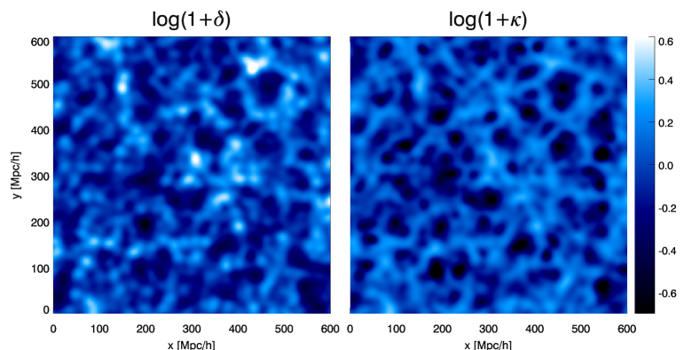
Figure 1: The left panel shows a slice of the original density field $\delta(\bm{x})$ smoothed on 8 Mpc/$h$ in $x-y$ plane. The right panel shows the corresponding slice of the reconstructed density field $\kappa(\bm{x})$, also smoothed on 8 Mpc/$h$.

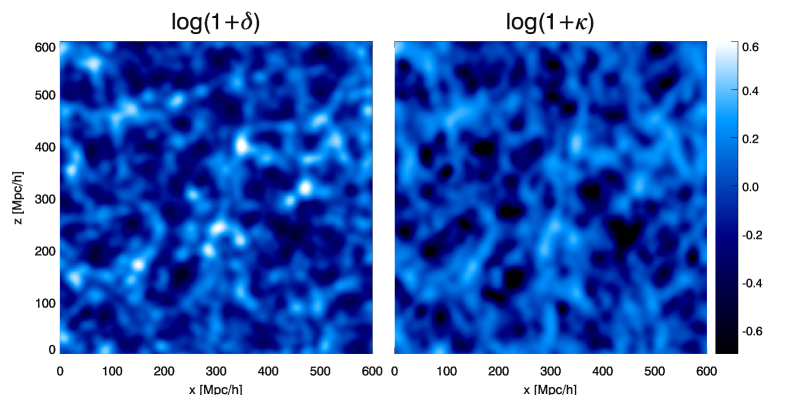
Figure 2: The left panel shows a slice of the original density field $\delta(\bm{x})$ smoothed on 8 Mpc/$h$ in $x-z$ plane. The right panel shows the corresponding slice of the reconstructed density field $\kappa(\bm{x})$, also smoothed on 8 Mpc/$h$.

In Fig. 1, we show a $1.17\ \mathrm{Mpc/}h$ slice of the original density field in the $x-y$ plane in the left panel and a slice of the reconstructed density field in the right panel, both smoothed on $8\ \mathrm{Mpc}/h$ to reduce the small-scale noise in order to make visual comparisons. In Fig. 2 we show the similar slices in the $x-z$ plane. We find in both cases the reconstructed density fields resemble the original ones. However, the strong peaks in the original density field are less prominent in the reconstructed field. The peaks in the original density field correspond to strongly nonlinear structures, like some very massive halos. In deriving Eq.(31), we assume that the small-scale density fluctuations undergo linear evolutions and the local anisotropies are due to the long-wavelength tidal field. However, the self-gravitational interaction is very strong around these nonlinear structures, so they change little under the weak gravitational interaction with the long-wavelength tidal field. Equation (31) does not hold in these regimes. The reconstruction exploits the nonlinear coupling between the long-wavelength tidal field and the small-scale density fluctuations but limited by the strong nonlinear gravitational clustering on small scales during structure formation, which leads to non-Gaussianity. Indeed, the original density field needs to be smoothed and Gaussianized to reduce the weighting of such contributions in order to obtain good reconstruction results.

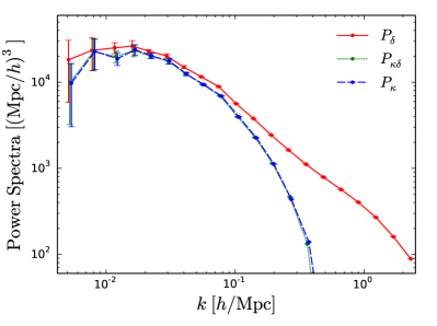
Figure 3: The auto and cross power spectra of the original and reconstructed density fields.

In Fig. 3, we show the auto power spectra of the original field $\delta$, the reconstructed field $\kappa$ and the cross power spectrum between $\kappa$ and $\delta$. Data points in the same $k$-bin are shifted slightly for clarity of display. The large errors at $k\sim 0.005\ h/{\rm Mpc}$ are due to finite modes on the largest scales. We see a good cross correlation between the original and reconstructed density fields over a wide range of wave numbers, $0.008\ h/{\rm Mpc}\lesssim k\lesssim 0.1\ h/{\rm Mpc}$. The general shape of $P_{\kappa}$ is similar to that of $P_{\delta}$. The power spectrum for $\kappa$ and the cross power spectrum between $\kappa$ and $\delta$ are nearly the same in this range because after we apply the Wiener filter to the reconstructed noisy field $\kappa_{\mathrm{3D}}$, the part correlated with $\delta$ remains in the clean field $\kappa$. At $k>0.1{\rm Mpc}/h$, the auto power spectrum of $\kappa$ and the cross power spectrum drop more rapidly than the original density field.

In Fig. 4, we plot the cross-correlation coefficient between the original density field and reconstructed density field,

$$r_{\kappa\delta}={P_{\kappa\delta}}/{\sqrt{P_{\delta}P_{\kappa}}}.$$ (61)

The error bars are estimated by the bootstrap resampling method. The cross-correlation coefficient $r_{\kappa\delta}$ is larger than 0.9 for $0.008\ h/{\rm Mpc}\lesssim k\lesssim 0.1\ h/{\rm Mpc}$. The cross-correlation coefficient drops rapidly at $k>0.1\ {\rm Mpc}/h$ because the reconstruction ceases to work on small scales.

IV.2 Dependence on smoothing scales and Gaussianization methods

To quantify the dependence on the smoothing scale, we perform reconstruction with three more smoothing scales, $R=2.5$, 5, and $10\ \mathrm{Mpc}/h$. Figure 4 shows the cross-correlation coefficients. The cross-correlation coefficients decrease when the smoothing scales are increased. We are using the small-scale structures to reconstruct the large-scale density field. When we increase the smoothing scale, we are losing the small-scale structures that can be used to provide cosmological information about the large-scale density field. However, the reconstruction results do not degrade significantly until the smoothing scale goes beyond $5\ \mathrm{Mpc}/h$, roughly the scale on which the structure growth transits from linear to nonlinear. The reconstruction is not sensitive to the smoothing scale unless we smooth on the linear scales.

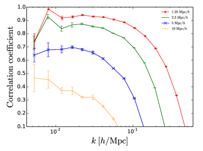
Figure 4: The cross-correlation coefficients for four different smoothing scales, $R=1.25$, 2.5, 5, and 10 $\mathrm{Mpc}/h$. The cross-correlation coefficients decrease when the smoothing scales are increased.

The logarithmic transform plays an important role in the cosmic tidal reconstruction. In Fig. 5, we also plot the result for a reconstruction without the logarithmic transform. The cross-correlation of the reconstructed field with the original field is much weaker than the one with the logarithmic transform and quickly drops to nearly zero when the wave number increases. Then, we adopt a different Gaussianization method by ranking the original density fluctuations into a Gaussian distribution Neyrinck et al. (2009) and perform tidal reconstruction using this normal density field. The cross-correlation coefficient is almost the same as that using the logarithmic transform. Apparently, the non-Gaussianity limits the shear reconstruction. The tidal shear estimators derived under the Gaussian assumption are not necessarily optimal for the non-Gaussian density field. The logarithmic transform reduces the non-Gaussianity of the density field so that a better result is achieved. It also fixes the displacement-density relation significantly as shown in Ref. Falck et al. (2012).

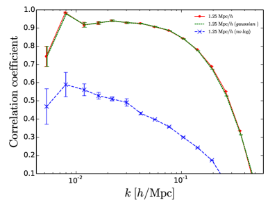
Figure 5: The cross-correlation coefficients for different Gaussianization methods. The solid line shows the reconstruction with the logarithmic transform. The dotted line shows the reconstruction using the normal density field. The dashed line shows the reconstruction without the logarithmic transform. The cross-correlation coefficients for the reconstruction with the logarithmic transform and the normal density field are almost the same.

IV.3 The anisotropic noise

The noise of $\kappa_{\mathrm{3D}}(\bm{k})$ is anisotropic as we discussed earlier. We show the anisotropic noise power spectrum in Fig. 6. The noises for modes with large $k_{\parallel}$ and small $k_{\perp}$ are orders of magnitude larger than other modes. This result confirms the estimate of noise derived from theory, $\sigma^{2}_{\kappa_{\mathrm{3D}}}\propto(k^{2}/k_{\perp}^{2})^{2}$, which diverges for small $k_{\perp}$. In Fig. 7, we show the anisotropic cross-correlation coefficient $r_{\kappa\delta}(k_{\parallel},k_{\perp})=P_{\kappa\delta}(k_{\parallel},k_{\perp})/\sqrt{P_{\delta}(k_{\parallel},k_{\perp})P_{\kappa}(k_{\parallel},k_{\perp})}$. The correlation between the original and reconstructed fields is better at the lower right corner, which can be close to 1 for modes with small $k_{\parallel}$, but drops quickly when $k_{\parallel}$ increases; the modes with large $k_{\parallel}$ and small $k_{\perp}$ are poorly reconstructed.

In Fig. 8, we show the anisotropic bias factor. The bias factor is nearly constant except for modes with very large $k_{\parallel}$ and very small $k_{\perp}$. Here, $b(k_{\parallel},k_{\perp})$ saturates at the upper left corner. Since these modes are noisy, the extremely large values of the bias at that corner are not reliable. This constancy of the bias factor shows that our reconstructed density field is a faithful representation of the original density field. It is also encouraging for applying the reconstructed density field to do cross correlations with other tracers for beating down cosmic variances Seljak (2009); McDonald and Seljak (2009).

The anisotropy in reconstruction is due to the fact we only use tidal shear fields in the tangential plane. The changes of the long-wavelength density field $\delta_{L}$ along the line of sight are inferred indirectly from the variations of tidal shear fields $\gamma_{1}(\bm{x})$ and $\gamma_{2}(\bm{x})$ along $x_{\parallel}$ axis, so we cannot capture the rapid changes of the density field along $x_{\parallel}$ axis. By including tidal shear fields containing derivatives with respect to $x_{\parallel}$ axis, the reconstruction will be improved. However, redshift space distortions will inevitably affect the reconstruction result. We leave the detailed study of this to a future paper.

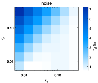
Figure 6: The anisotropic noise power spectrum $P_{n}(k_{\parallel},k_{\perp})$. The noises for modes with large $k_{\parallel}$ and small $k_{\perp}$ are orders of magnitude larger than other modes.

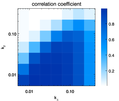
Figure 7: The cross-correlation coefficient $r_{\kappa\delta}(k_{\parallel},k_{\perp})$. The cross-correlation is better at the lower right corner, which can be close to 1 for modes with small $k_{\parallel}$, but drops quickly when $k_{\parallel}$ increases; the modes with large $k_{\parallel}$ and small $k_{\perp}$ are poorly reconstructed.

V Discussions

In this paper, we show how the long-wavelength tidal field $t_{ij}$ can be reconstructed from the local small-scale power spectrum. To reconstruct $t_{ij}$ from the anisotropic small-scale density perturbations, we need to learn the interaction process clearly. In this paper, we follow the treatments in Ref. Schmidt et al. (2014), only considering the coupling between $\mathbf{s}_{1s}$ and $\mathbf{s}_{1t}$, which is the leading-order effect from $t_{ij}$. However, unlike weak lensing, where the interaction is weak so that the linearized calculation is good enough for most cases, the tidal interaction is inherently a nonlinear process. Higher-order terms of form $(\mathbf{s}_{1s})^{n}\mathbf{s}_{1t}$ $(n>1)$ also play important roles in the tidal interaction, as the nonlinearities on small scales are quite strong. The proportional coefficient in Eq. (32) will change if we include terms like $(\mathbf{s}_{1s})^{n}\mathbf{s}_{1t}$ $(n>1)$. The tidal shear estimators we used in this paper are biased since we do not know the tidal interaction process accurately. However, even if we include some higher-order terms, the constructed estimators might still be biased, as this still does not describe the full nonlinear process. In this paper, we assume that the nonlinearities only change the proportional coefficient $f(k,\tau)$. The tidal distortion of the local power spectrum is still proportional to $\hat{k}^{i}\hat{k}^{j}t_{ij}^{(0)}$, and the proportional coefficient does not vary significantly over different wave numbers. Then, we can absorb the unknown coefficient into the bias factor introduced in Eq. (43). The bias factor can be solved from $N$-body simulations. The proportional constant from the Poisson equation and the normalization constant $Q$ in the tidal shear estimators can also be absorbed in this bias factor. The integral for $Q$ in Eq.(53) would diverge at large $k$ if there were no noise in the power spectrum $P(k)$, i.e., $P(k)=P_{\mathrm{tot}}(k)$. This happens when we use the dark matter density field from high precision $N$-body simulations to reconstruct the large-scale density field. The bias factor solves this problem. The result can be improved in the future by including the higher-order perturbations. Nevertheless, the reconstruction works well even at this leading order, with the cross-correlation coefficient larger than 0.9 until $k\gtrsim 0.1\mathrm{Mpc}/h$. The reconstruction should work even better at higher redshifts since Eq. (31) holds better when the small-scale density fluctuations undergo less nonlinear evolutions.

Figure 8: The bias factor $b(k_{\parallel},k_{\perp})$. The bias factor is almost scale independent in this plane. $b(k_{\parallel},k_{\perp})$ saturates at the upper left corner. Since these modes are noisy, the extremely large values of the bias at that corner are not reliable.

The $\hat{\gamma}_{1}$ and $\hat{\gamma}_{2}$ estimators are optimal under the Gaussian assumption, while this is not the real case. The non-Gaussian density field is treated as a Gaussian random field throughout the reconstruction. So we need to Gaussianize the non-Gaussian density field or the correlation would be rather weak. It would be worthwhile to investigate the optimal estimators for non-Gaussian sources, which can be constructed from $N$-body simulations.

There is still one more limitation in the reconstruction. The $\hat{\gamma}_{1}$ and $\hat{\gamma}_{2}$ estimators are unbiased and of minimum variance in the long-wavelength limit, providing optimal tidal shear reconstructions. However, at larger wave numbers, the tidal shear field would be underestimated by a scale-dependent multiplicative bias factor which needs to be corrected Lu and Pen (2008); Bucher et al. (2012). In this paper, we find the estimator derived in the long-wavelength limit still works well if we only use the reconstruction modes with scale larger than the smoothing scale. However, when there is an overlap between these two scales, the reconstruction result would degrade. A more sophisticated method is needed in that case.

In this paper, we use the dark matter density field directly to reconstruct the large-scale density field. However, the actual tracers would be galaxies, which are located inside dark matter halos which are in turn distributed in the underlying dark matter density field. Due to the discreteness of the galaxy (halo) field, the tidal reconstruction may not be as good as that of the dark matter field. The scale-dependent galaxy (halo) bias may also complicate the reconstruction procedure. Further, the reconstruction will be affected by the tidal galaxy (halo) bias. These effects can be quantified using the halo density fields from $N$-body simulations. We plan to study these in the future.

The reconstruction method developed in this paper has great potential applications. The reconstructed field $\kappa$ gives the distribution of dark matter on large scales. By cross correlating with the original galaxy (halo) field, we can measure the logarithmic growth rate without sample variance McDonald and Seljak (2009). This can potentially provide high precision measurements of neutrino masses and tests of gravity. The reconstructed field $\kappa$ is also important for measuring the dark matter-neutrino cross-correlation dipole Zhu et al. (2014). Moreover, it is also important in the case where the measurement of long-wavelength modes is missing or has large noise. In the 21cm intensity mapping survey Chang et al. (2008), modes with small radial wave numbers are seriously contaminated by foreground radiation and are often subtracted in data analysis. This makes it difficult or even impossible to do cross correlations with surveys which only probe the long-wavelength radial modes, including weak lensing, photo-$z$ galaxies, integrated Sachs-Wolf effect and kinetic Sunyaev-Zel’dovich effect. Since cosmic tidal reconstruction can recover the long-wavelength radial modes, it enables the cross correlations of the 21cm intensity survey with other cosmic probes. For 21cm intensity mapping experiments such as Tianlai Chen (2012); Xu et al. (2015) and CHIME Bandura et al. (2014), the cosmic tidal reconstruction method can be very useful.

References

- Schmidt et al. (2014) F. Schmidt, E. Pajer, and M. Zaldarriaga, Phys. Rev. D 89, 083507 (2014), eprint 1312.5616.
- Li et al. (2014) Y. Li, W. Hu, and M. Takada, Phys. Rev. D 90, 103530 (2014), eprint 1408.1081.
- Pen et al. (2012) U.-L. Pen, R. Sheth, J. Harnois-Deraps, X. Chen, and Z. Li, ArXiv e-prints (2012), eprint 1202.5804.
- Lu and Pen (2008) T. Lu and U.-L. Pen, MNRAS 388, 1819 (2008), eprint 0710.1108.
- Lu et al. (2010) T. Lu, U.-L. Pen, and O. Doré, Phys. Rev. D 81, 123015 (2010), eprint 0905.0499.
- Furlanetto and Lidz (2007) S. R. Furlanetto and A. Lidz, ApJ 660, 1030 (2007), eprint astro-ph/0611274.
- Adshead and Furlanetto (2008) P. J. Adshead and S. R. Furlanetto, MNRAS 384, 291 (2008), eprint 0706.3220.
- Morales et al. (2012) M. F. Morales, B. Hazelton, I. Sullivan, and A. Beardsley, ApJ 752, 137 (2012), eprint 1202.3830.
- Masui and Pen (2010) K. W. Masui and U.-L. Pen, Physical Review Letters 105, 161302 (2010), eprint 1006.4181.
- Jeong and Kamionkowski (2012) D. Jeong and M. Kamionkowski, Physical Review Letters 108, 251301 (2012), eprint 1203.0302.
- Falck et al. (2012) B. L. Falck, M. C. Neyrinck, M. A. Aragon-Calvo, G. Lavaux, and A. S. Szalay, ApJ 745, 17 (2012), eprint 1111.4466.
- Eardley et al. (1973) D. M. Eardley, D. L. Lee, A. P. Lightman, R. V. Wagoner, and C. M. Will, Physical Review Letters 30, 884 (1973).
- Li et al. (2016) Y. Li, W. Hu, and M. Takada, Phys. Rev. D 93, 063507 (2016), eprint 1511.01454.
- Lazeyras et al. (2016) T. Lazeyras, C. Wagner, T. Baldauf, and F. Schmidt, J. Cosmology Astropart. Phys 2, 018 (2016), eprint 1511.01096.
- Baldauf et al. (2015) T. Baldauf, U. Seljak, L. Senatore, and M. Zaldarriaga, ArXiv e-prints (2015), eprint 1511.01465.
- Kaiser and Squires (1993) N. Kaiser and G. Squires, ApJ 404, 441 (1993).
- Zaldarriaga and Seljak (1999) M. Zaldarriaga and U. Seljak, Phys. Rev. D 59, 123507 (1999), eprint astro-ph/9810257.
- Bucher et al. (2012) M. Bucher, C. S. Carvalho, K. Moodley, and M. Remazeilles, Phys. Rev. D 85, 043016 (2012), eprint 1004.3285.
- Harnois-Déraps et al. (2013) J. Harnois-Déraps, U.-L. Pen, I. T. Iliev, H. Merz, J. D. Emberson, and V. Desjacques, MNRAS 436, 540 (2013), eprint 1208.5098.
- Neyrinck et al. (2009) M. C. Neyrinck, I. Szapudi, and A. S. Szalay, ApJ 698, L90 (2009), eprint 0903.4693.
- Seljak (2009) U. Seljak, Physical Review Letters 102, 021302 (2009), eprint 0807.1770.
- McDonald and Seljak (2009) P. McDonald and U. Seljak, J. Cosmology Astropart. Phys 10, 007 (2009), eprint 0810.0323.
- Zhu et al. (2014) H.-M. Zhu, U.-L. Pen, X. Chen, D. Inman, and Y. Yu, Physical Review Letters 113, 131301 (2014), eprint 1311.3422.
- Chang et al. (2008) T.-C. Chang, U.-L. Pen, J. B. Peterson, and P. McDonald, Physical Review Letters 100, 091303 (2008), eprint 0709.3672.
- Chen (2012) X. Chen, International Journal of Modern Physics Conference Series 12, 256 (2012), eprint 1212.6278.
- Xu et al. (2015) Y. Xu, X. Wang, and X. Chen, ApJ 798, 40 (2015), eprint 1410.7794.
- Bandura et al. (2014) K. Bandura, G. E. Addison, M. Amiri, J. R. Bond, D. Campbell-Wilson, L. Connor, J.-F. Cliche, G. Davis, M. Deng, N. Denman, et al., in Society of Photo-Optical Instrumentation Engineers (SPIE) Conference Series (2014), vol. 9145 of Society of Photo-Optical Instrumentation Engineers (SPIE) Conference Series, p. 22, eprint 1406.2288.