Constructing functions with prescribed
pathwise quadratic variation

Abstract

We construct rich vector spaces of continuous functions with prescribed curved or linear pathwise quadratic variations. We also construct a class of functions whose quadratic variation may depend in a local and nonlinear way on the function value. These functions can then be used as integrators in Föllmer’s pathwise Itō calculus. Our construction of the latter class of functions relies on an extension of the Doss–Sussman method to a class of nonlinear Itō differential equations for the Föllmer integral. As an application, we provide a deterministic variant of the support theorem for diffusions. We also establish that many of the constructed functions are nowhere differentiable.

Keywords: Pathwise quadratic variation, Föllmer integral, pathwise Itō differential equation, Doss–Sussman method, support theorem, nowhere differentiability

1 Introduction

In the seminal paper [14], H. Föllmer provided a strictly pathwise approach to Itō’s formula. The formula is “pathwise” in the sense that integrators are fixed, nonstochastic functions $x:[0,1]\to\mathbb{R}$ that do not need to arise as typical sample paths of a semimartingale. It thus became clear that Itō’s formula is essentially a second-order extension of the fundamental theorem of calculus for Stieltjes integrals. A systematic introduction to pathwise Itō calculus, including an English translation of [14], is provided in [30].

In recent years, there has been an increased interest in pathwise Itō calculus. On the one hand, this increase is due to a growing sensitivity to model risk in mathematical finance and economics and the ensuing aspiration to construct dynamic trading strategies without reliance on a probabilistic model. As a matter of fact, a number of recent case studies have shown that some nontrivial results of this type can be obtained by means of pathwise Itō calculus; see, e.g., [1; 2; 6; 15; 23; 26; 28; 34]. On the other hand, the recent functional extension of Föllmer’s pathwise Itō formula by Dupire [9] and Cont and Fournié [4; 5] facilitated new and exciting mathematical developments such as the theory of viscosity solution of partial differential equations on infinite-dimensional path space [10; 11].

A function $x\in C[0,1]$ can be used as an integrator in Föllmer’s pathwise Itō calculus if it admits a continuous pathwise quadratic variation $t\mapsto\langle x\rangle_{t}$ along a given refining sequence of partitions of $[0,1]$. It is, however, not entirely straightforward to construct functions with a given, nontrivial quadratic variation. Of course, one can use the sample paths of a continuous semimartingale, but these will satisfy the requirement only in an almost sure sense, and it will not be possible to determine whether a particular sample path will be as desired or belong to the nullset of trajectories for which the quadratic variation does not exist. Based on results by Gantert [17; 18], a set $\mathscr{X}\subset C[0,1]$ was constructed in [27] for which each element $x\in\mathscr{X}$ has the linear quadratic variation $\langle x\rangle_{t}=t$. This set, however, has the disadvantage that the quadratic variation of the sum of $x,y\in\mathscr{X}$ need not exist. The existence of $\langle x+y\rangle$ is equivalent to the existence of the covariation $\langle x,y\rangle$ and is crucial for multidimensional pathwise Itō calculus.

In this note, our goal is to construct rich classes of functions with prescribed pathwise quadratic variation so that these functions can serve as test integrators for pathwise Itō calculus. More precisely, we will construct the following three classes of functions.

1. A vector space of functions $x$ with the (curved) quadratic variation $\langle x\rangle_{t}=\int_{0}^{t}f^{2}(s)\,ds$ for all $t$, where $f$ is a certain Riemann integrable function associated with $x$.

2. A vector space of functions $y$ with the (linear) quadratic variation $\langle y\rangle_{t}=t\int_{0}^{1}f^{2}(s)\,ds$ for all $t$, where $f$ is again a certain Riemann integrable function associated with $y$.

3. A class of functions $z$ with the “local” quadratic variation $\langle z\rangle_{t}=\int_{0}^{t}\sigma^{2}(s,z(s))\,ds$ for some sufficiently regular “volatility” function $\sigma$.

The class in (C) was first postulated and used by Bick and Willinger [2]; see also  [23; 29]. Our corresponding result now establishes a path-by-path construction of such functions without the need to rely on selection from the sample paths of a diffusion process.

Note that, unlike in the case of stochastic processes, it is not possible to construct the functions in (A) and (C) from functions with linear quadratic variation via time change, because a time-changed function will generally only admit a quadratic variation with respect to a time-changed sequence of partitions. By contrast, our construction of the vector spaces in (A) and (B) relies on Proposition 2.1, which combines an observation by Gantert [17; 18] with the Stolz–Cesaro theorem so as to characterize the existence of quadratic variation along the sequence of dyadic partitions by means of the convergence of certain Riemann sums. This argument yields the set in (A) relatively directly, while the set in (B) requires the additional use of an ergodic shift and Weyl’s equidistribution theorem. We also prove that many functions in (A) and (B) are nowhere differentiable. The set in (C) will be constructed by solving a pathwise Itō differential equation for the Föllmer integral by means of the Doss–Sussman method, where the Itō differential equation is driven by a function from the set in (B). We will then show that the set in (C) is sufficiently rich in the sense that it is dense in $C[0,1]$ and that its members can connect any two points within any given time interval. This latter result can be regarded as a deterministic variant of a support theorem for diffusion processes as in [31].

This paper is structured as follows. Preliminary definitions and results, including the above-mentioned Proposition 2.1, are collected in Section 2.1. The sets in (A) and (B) are constructed in Section 2.2. The existence and uniqueness theorem for pathwise Itō differential equations, from which the functions in (C) can be obtained, and the corresponding “support theorem” are stated in Section 2.3. All proofs are deferred to Section 3.

2 Main results

2.1 Preliminaries

A partition of the interval $[0,1]$ will be a finite set $\mathbb{T}=\{t_{0},t_{1},\dots,t_{n}\}$ such that $0=t_{0}<t_{1}<\cdots<t_{n}=1$. Now let $(\mathbb{T}_{n})_{n\in\mathbb{N}}$ be an increasing sequence of partitions $\mathbb{T}_{1}\subset\mathbb{T}_{2}\subset\cdots$ of the interval $[0,1]$ such that the mesh of $\mathbb{T}_{n}$ tends to zero; such a sequence $(\mathbb{T}_{n})_{n\in\mathbb{N}}$ will be called a refining sequence of partitions. A typical example will be the sequence of dyadic partitions,

$$\mathbb{T}_{n}:=\{k2^{-n}\,|\,n\in\mathbb{N},k=0,\dots,2^{n}\},\qquad n=0,1,\dots$$ (2.1)

It will be convenient to denote by $s^{\prime}$ the successor of $s$ in $\mathbb{T}_{n}$, i.e.,

$$s^{\prime}=\begin{cases}\min\{t\in\mathbb{T}_{n}\,|\,t>s\}&\text{if $s<1$,}\\ 1&\text{if $s=1$.}\end{cases}$$

For $x\in C[0,1]$ one then defines the sequence

$$\langle x\rangle_{t}^{n}:=\sum_{s\in\mathbb{T}_{n},\,s\leq t}(x(s^{\prime})-x(s))^{2}.$$

We will say that $x$ admits the quadratic variation $\langle x\rangle_{t}$ along $(\mathbb{T}_{n})$ and at $t\in[0,1]$ if the limit

$$\langle x\rangle_{t}:=\lim_{n\uparrow\infty}\langle x\rangle^{n}_{t}$$ (2.2)

exists. Since the sequence $\langle x\rangle^{n}_{t}$ need not be monotone in $n$, it is not clear a priori whether the limit in (2.2) exists for any fixed $t\in[0,1]$. Moreover, even if the limit exists, it may depend strongly on the particular choice of the underlying sequence of partitions; see, e.g., [16, p. 47] and [27, Proposition 2.7]. For $x,y\in C[0,1]$, let

$$\langle x,y\rangle_{t}^{n}:=\sum_{s\in\mathbb{T}_{n},\,s\leq t}(x(s^{\prime})-x(s))(y(s^{\prime})-y(s))$$

and observe that

$$\langle x,y\rangle_{t}^{n}=\frac{1}{2}\Big{(}\langle x+y\rangle_{t}^{n}-\langle x\rangle_{t}^{n}-\langle y\rangle_{t}^{n}\Big{)}.$$ (2.3)

If $x$ and $y$ admit the quadratic variations $\langle x\rangle_{t}$ and $\langle y\rangle_{t}$, then it follows from (2.3) that the covariation of $x$ and $y$,

$$\langle x,y\rangle_{t}:=\lim_{n\uparrow\infty}\langle x,y\rangle_{t}^{n},$$

exists at $t$ if and only if $\langle x+y\rangle_{t}$ exists. This, however, need not be the case even if both $\langle x\rangle_{t}$ and $\langle y\rangle_{t}$ exist; see [27, Proposition 2.7] for an example. It follows in particular that the class of all functions $x$ that admit the quadratic variation $\langle x\rangle_{t}$ along $(\mathbb{T}_{n})_{n\in\mathbb{N}}$ is not a vector space. The main goal of this paper will be to construct sufficiently large classes of functions with prescribed quadratic variation and such that $\langle x,y\rangle_{t}$ exists for all $t$ and all $x,y$ in this class so that this class is indeed a vector space.

As observed by Gantert [17; 18], the quadratic variation of a function $x\in C[0,1]$ along the sequence of dyadic partitions (2.1) is closely related to its development in terms of the Faber–Schauder functions, which are defined as

$$e_{\emptyset}(t):=t,\qquad e_{0,0}(t):={\max\{0,\min\{t,1-t\}\}},\qquad e_{n,k}(t):=2^{-n/2}e_{0,0}(2^{n}t-k)$$

for $t\in\mathbb{R}$, $n=1,2,\dots$, and $k\in\mathbb{Z}$. The graph of $e_{n,k}$ looks like a wedge with height $2^{-\frac{n+2}{2}}$, width $2^{-n}$, and center at $t=(k+\frac{1}{2})2^{-n}$. In particular, the functions $e_{n,k}$ have disjoint support for distinct $k$ and fixed $n$. It is well known that every $x\in C[0,1]$ can be uniquely represented by means of the following uniformly convergent series,

$$x=x(0)+{(x(1)-x(0))}e_{\emptyset}+\sum_{m=0}^{\infty}\sum_{k=0}^{2^{m}-1}\theta_{m,k}e_{m,k},$$ (2.4)

where the coefficients $\theta_{m,k}$ are given as

$$\theta_{m,k}=2^{m/2}\bigg{(}2x\Big{(}\frac{2k+1}{2^{m+1}}\Big{)}-x\Big{(}\frac{k}{2^{m}}\Big{)}-x\Big{(}\frac{k+1}{2^{m}}\Big{)}\bigg{)};$$

see, e.g., [22, p.3]. Since in this note we are only dealing with functions on $[0,1]$, we will only need the Faber–Schauder functions $e_{n,k}$ for $k=0,\dots,2^{n}-1$ and their domain of definition can be restricted to $[0,1]$. For $t=1$, the equivalence of conditions (a) and (b) in the following proposition was stated in [18, Lemma 1.1 (ii)].

Proposition 2.1.

Let $x\in C[0,1]$ have Faber–Schauder development (2.4) and let $(\mathbb{T}_{n})$ be the sequence of dyadic partitions. Then, for $t\in\bigcup_{n}\mathbb{T}_{n}$, the following conditions are equivalent.

1. The quadratic variation $\langle x\rangle_{t}$ exists.

2. The following limit exists,

   $$\ell_{1}(t):=\lim_{n\uparrow\infty}\frac{1}{2^{n}}\sum_{m=0}^{n-1}\sum_{k=0}^{\lfloor(2^{m}-1)t\rfloor}\theta_{m,k}^{2}.$$

3. The following limit exists,

   $$\ell_{2}(t):=\lim_{n\uparrow\infty}\frac{1}{2^{n}}\sum_{k=0}^{\lfloor(2^{n}-1)t\rfloor}\theta_{n,k}^{2}.$$

In this case, we furthermore have $\langle x\rangle_{t}=\ell_{1}(t)=\ell_{2}(t)$.

Remark 2.2.

Let $y\in C[0,1]$ have the Faber–Schauder development

$$y=y(0)+{(y(1)-y(0))}e_{\emptyset}+\sum_{m=0}^{\infty}\sum_{k=0}^{2^{m}-1}\vartheta_{m,k}e_{m,k}.$$ (2.5)

Then it follows from Proposition 2.1 and polarization (2.3) that the covariation $\langle x,y\rangle_{t}$ exists along the sequence of dyadic partitions and for $t\in\bigcup_{n}\mathbb{T}_{n}$ if and only if the limit

$$\ell(t)=\lim_{n\uparrow\infty}\frac{1}{2^{n}}\sum_{k=0}^{\lfloor(2^{n}-1)t\rfloor}\theta_{n,k}\vartheta_{n,k}$$

exists and that, in this case, $\langle x,y\rangle_{t}=\ell(t)$.

We emphasize that the formulas for $\langle x\rangle_{t}$ and $\langle x,y\rangle_{t}$ obtained in Proposition 2.1 and Remark 2.2 are only valid if quadratic variation is considered along the sequence $(\mathbb{T}_{n})$ of dyadic partitions (2.1), because it is naturally related to the Faber–Schauder development of continuous functions. In principle, it should be possible to obtain similar results also for other wavelet expansions, which would correspond to other sequences of partitions, such as general $p$-adic partitions. Such an analysis is, however, beyond the scope of this paper.

Remark 2.3.

Let $x,y\in C[0,1]$ have Faber–Schauder developments (2.4) and (2.5) with coefficients $\theta_{n,k},\vartheta_{n,k}\in\{-1,+1\}$ for all $n$ and $k$. Then

$$\frac{1}{2^{n}}\sum_{k=0}^{\lfloor(2^{n}-1)t\rfloor}\theta_{n,k}\vartheta_{n,k}=\frac{{\lfloor(2^{n}-1)t\rfloor+1}}{2^{n}}-\frac{2}{2^{n}}\sum_{k=0}^{\lfloor(2^{n}-1)t\rfloor}1_{\{\theta_{n,k}\neq\vartheta_{n,k}\}}=\frac{{\lfloor(2^{n}-1)t\rfloor+1}}{2^{n}}-2\nu_{n}(t),$$

where

$$\nu_{n}(t):=\frac{1}{2^{n}}\text{card}\big{\{}0\leq k\leq\lfloor(2^{n}-1)t\rfloor\,\big{|}\,\theta_{n,k}\neq\vartheta_{n,k}\big{\}}$$

is the frequency of non-coincidence. Since ${\lfloor(2^{n}-1)t\rfloor}{2^{-n}}\to t$, it follows that $\langle x,y\rangle_{t}$ exists if and only if the frequency $\nu_{n}(t)$ converges to a limit $\nu(t)\in[0,1]$.

2.2 Constructing vector spaces of functions with prescribed curved and linear quadratic variation

We start by constructing a vector space of functions with curved quadratic variation along the sequence (2.1) of dyadic partitions. To this end, we let $\mathscr{F}$ denote the class of all sequences $\bm{f}=(f_{n})_{n=0,1,\dots}$ of bounded functions $f_{n}:[0,1]\to\mathbb{R}$ that converge uniformly to a Riemann integrable function $f_{\infty}:=\lim_{n}f_{n}$. For $\bm{f}\in\mathscr{F}$, we define

$$\theta_{n,k}(\bm{f}):=f_{n}(k2^{-n})$$

and

$$x_{\bm{f}}:=\sum_{n=0}^{\infty}\sum_{k=0}^{2^{n}-1}\theta_{n,k}(\bm{f})e_{n,k}.$$

The preceding sum converges absolutely since the coefficients $\theta_{n,k}(\bm{f})$ are uniformly bounded. As a matter of fact, the boundedness of the coefficients implies that $x_{\bm{f}}$ is even Hölder continuous with exponent $1/2$; see  [3, Theorem 1]. It follows in particular that the class $\{x_{\bm{f}}\,|\,\bm{f}\in\mathscr{F}\}$ does not contain the typical sample paths of a continuous semimartingale with nonvanishing quadratic variation.

Proposition 2.4.

Let $(\mathbb{T}_{n})$ be the sequence (2.1) of dyadic partitions. Then the following assertions hold.

1. If $\bm{f}\in\mathscr{F}$, then $x_{\bm{f}}$ admits the continuous quadratic variation $\langle x_{\bm{f}}\rangle_{t}=\int_{0}^{t}f^{2}_{\infty}(s)\,ds$ for all $t\in[0,1]$.

2. If $\bm{f},\bm{g}\in\mathscr{F}$, then $x_{\bm{f}}$ and $x_{\bm{g}}$ admit the continuous covariation $\langle x_{\bm{f}},x_{\bm{g}}\rangle_{t}=\int_{0}^{t}f_{\infty}(s)g_{\infty}(s)\,ds$ for all $t\in[0,1]$.

In particular, the class $\{x_{\bm{f}}\,|\,\bm{f}\in\mathscr{F}\}$ is a vector space of functions admitting a continuous quadratic variation.

See Figure 1 for an illustration of functions in $x_{\bm{f}}$. We continue with a non-differentiability result. Recall that, by Lebesgue’s criterion [25, Theorem 11.33], a function $f:[0,1]\to\mathbb{R}$ is Riemann integrable if and only if it is bounded and continuous almost everywhere.

Proposition 2.5.

For any $\bm{f}\in\mathscr{F}$, the function $x_{\bm{f}}$ is not differentiable at any continuity point, $t$, of $f_{\infty}$ for which $f_{\infty}(t)\neq 0$. In particular, $x_{\bm{f}}$ is not differentiable almost everywhere on $\{f_{\infty}\neq 0\}$.

Now we will construct a rich vector space of functions possessing a linear quadratic variation. It was shown in [27] that all functions $x$ whose Faber–Schauder coefficients take only the values $\pm 1$ have the linear quadratic variation $\langle x\rangle_{t}=t$ for all $t$, but the corresponding class, $\mathscr{X}$, is not a vector space. For our construction, we let

$$t\text{\,mod\,}1:=t-\lfloor t\rfloor$$

denote the fractional part of $t\geq 0$. For $\bm{f}\in\mathscr{F}$ and $\alpha>0$, we define

$$\vartheta_{n,k}(\alpha,\bm{f}):=f_{n}\big{(}\alpha k\text{\,mod\,}1\big{)}$$

and

$$y_{\alpha}^{\bm{f}}:=\sum_{n=0}^{\infty}\sum_{k=0}^{2^{n}-1}\vartheta_{n,k}(\alpha,\bm{f})e_{n,k}.$$

Again, the preceding sum converges absolutely, as all coefficients $\vartheta_{n,k}(\alpha,\bm{f})$ are bounded. Moreover, $y_{\alpha}^{\bm{f}}$ is Hölder continuous with exponent $1/2$.

Proposition 2.6.

Let $(\mathbb{T}_{n})$ be the sequence of dyadic partitions and $\alpha>0$ be irrational and fixed. Then the following assertions hold.

1. If $\bm{f}\in\mathscr{F}$, then $y_{\alpha}^{\bm{f}}$ admits the linear quadratic variation $\langle y_{\alpha}^{\bm{f}}\rangle_{t}=t\int_{0}^{1}f_{\infty}^{2}(s)\,ds$ for $t\in[0,1]$.

2. If $\bm{f},\bm{g}\in\mathscr{F}$, then $y_{\alpha}^{\bm{f}}$ and $y_{\alpha}^{\bm{g}}$ admit the linear covariation $\langle y_{\alpha}^{\bm{f}},y_{\alpha}^{\bm{g}}\rangle_{t}=t\int_{0}^{1}f_{\infty}(s)g_{\infty}(s)\,ds$ for $t\in[0,1]$.

In particular, the class $\{y_{\alpha}^{\bm{f}}\,|\,\bm{f}\in\mathscr{F}\}$ is a vector space of functions admitting a linear quadratic variation.

An illustration of functions $y_{\alpha}^{\mathbf{f}}$ for various choices of $\alpha$ and $\mathbf{f}$ is given in Figure 2. When comparing Figures 1 and 2, one can see that the functions $y_{\alpha}^{\mathbf{f}}$ exhibit a lower degree of regularity and look more “random" than the functions $x_{\mathbf{f}}$. This effect is due to the ergodic behavior of the shift $x\mapsto(x+\alpha)\text{\,mod\,}1$, which underlies the coefficients $\vartheta_{n,k}(\alpha,\mathbf{f})$. The following non-differentiability result can be proved in the same way as Proposition 2.5.

Proposition 2.7.

Suppose the $\alpha>0$ is irrational and $\bm{f}\in\mathscr{F}$ is such that $|f_{\infty}|$ is bounded away from zero. Then $y_{\alpha}^{\bm{f}}$ is nowhere differentiable.

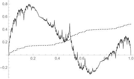
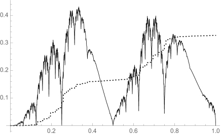
Figure 1: Plots of the functions $x_{\bm{f}}$ when $f_{n}(t):=\cos 2\pi t$ (left) and $f_{n}(t):=(\sin 7t)^{2}$ (right) for all $n$. The dotted lines correspond to $\langle x_{\bm{f}}\rangle^{7}$.

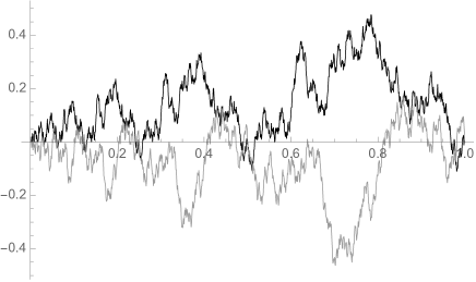
Figure 2: Plots of the functions $y_{\alpha}^{\bm{f}}$ when $\alpha=e$ (grey), $\alpha=10e$ (black), $f_{n}(t):=\sin 2\pi t$ (left), and $f_{n}(t):=\frac{10t-n}{1+n}\cos\frac{6\pi nt}{1+n}$ (right).

2.3 Constructing functions with local quadratic variation via pathwise Itō differential equations

In this section, $(\mathbb{T}_{n})$ may be any refining sequence of partitions; we do not insist that it is given by the dyadic partitions in (2.1). Bick’s and Willinger’s approach [2] to the strictly pathwise hedging of options relies on the following class of trajectories,

$$\Big{\{}z\in C[0,1]\,\Big{|}\,\text{$z$ admits the quadratic variation }\langle z\rangle_{t}=\int_{0}^{t}\beta(s,z(s))\,ds\text{ for all $t$}\Big{\}}.$$ (2.6)

Here, $\beta$ is a certain strictly positive function, playing the role of a squared local volatility. We will therefore refer to (2.6) as a set of functions with local quadratic variation. See also [23; 28; 29] for results involving sets of the form (2.6).

In the preceding sections and in [27], trajectories $x$ were constructed that have, e.g., the linear quadratic variation $\langle x\rangle_{t}=t$. A first guess how to construct a function in the set (2.6) from a given $x$ with linear quadratic variation could be to apply a time change as, e.g., in [12]. This does indeed yield a function with the desired quadratic variation—but a quadratic variation that is taken with respect to a time-changed sequence of partitions. It is not at all clear if the time-changed function $x$ will also admit a quadratic variation along the original refining sequence $(\mathbb{T}_{n})$, and even if it does, it is not clear if it is as desired. Thus, a time change is not an appropriate means of constructing functions in (2.6). Instead, our approach will be to set up and solve a corresponding Itō differential equation, whose solution will then belong to the set in (2.6).

The discussion of pathwise Itō differential equations is also interesting in its own right. It is based on Föllmer’s theory [14] of pathwise Itō integration for integrators that admit a continuous quadratic variation. By Föllmer’s pathwise Itō formula, the integral $\int_{0}^{t}\eta(s)\,dx(s)$ exists as a limit of non-anticipative Riemann sums for all $\eta$ from the class of admissible integrands, defined below. This pathwise integral is sometimes called the Föllmer integral. By $\text{\it CBV}[0,1]$ we will denote the class of continuous functions on $[0,1]$ that are of bounded variation. The following definition is taken from [26, Definition 11]; see [26, Section 3] for further details.

Definition 2.8.

Let $x\in C[0,1]$ be a function with continuous quadratic variation along $(\mathbb{T}_{n})$. A function $t\mapsto\eta(t)$ is called an admissible integrand for $x$ if there exist $n\in\mathbb{N}$, a continuous function $\mathbf{A}:[0,1]\to\mathbb{R}^{n}$ whose components belong to $\text{\it CBV}[0,1]$, an open set $U\subset\mathbb{R}^{n}\times\mathbb{R}$ with $(\mathbf{A}(t),x(t))\in U$ for all $t$, and a continuously differentiable function $f:U\to\mathbb{R}$ for which, for all $\bm{a}\in\{\bm{b}\in\mathbb{R}^{n}\,|\,\exists\xi\in\mathbb{R}\text{ s.th.\leavevmode\nobreak\ }(\bm{\mathbf{b}},\xi)\in U\}$, the function $\xi\mapsto f(\mathbf{a},\xi)$ is twice continuously differentiable on its domain, such that $\eta(t)=\frac{\partial}{\partial\xi}f(\mathbf{A}(t),x(t))$.

Remark 2.9.

Suppose that $x$ and $\mathbf{A}$ are as in Definition 2.8 and that $g\in C^{1}(\mathbb{R}^{n}\times\mathbb{R})$. Then $\eta(t):=g(\mathbf{A}(t),x(t))$ is an admissible integrand for $x$. This follows by taking $f(\mathbf{a},\xi):=\int_{0}^{\xi}g(\mathbf{a},y)\,dy$ in Definition 2.8. In particular, $\eta(t)=\exp\{\mu t+\sigma x(t)\}$, $\eta(t)=x^{n}(t)$, $\eta(t)=\exp\{x^{n}(t)\}$, $\eta(t)=\log(1+x^{2n}(t))$, or smooth functions thereof are admissible integrands for $\mu,\sigma\in\mathbb{R}$ and $n\in\mathbb{N}$.

We can now define the concept of a solution to a pathwise Itō differential equation.

Definition 2.10.

Suppose that $x\in C[0,1]$ is a function with continuous quadratic variation along $(\mathbb{T}_{n})$, $A$ belongs to $\text{\it CBV}[0,1]$, $\sigma:[0,1]\times\mathbb{R}\to\mathbb{R}$ and $b:[0,1]\times\mathbb{R}\to\mathbb{R}$ are continuous functions, and $z_{0}\in\mathbb{R}$. A function $z\in C[0,1]$ is called a solution of the Itō differential equation

$$dz(t)=\sigma(t,z(t))\,dx(t)+b(t,z(t))\,dA(t)$$ (2.7)

with initial condition $z(0)=z_{0}$ if $t\mapsto\sigma(t,z(t))$ is an admissible integrand for $x$ and $z$ satisfies the integral form of (2.7),

$$z(t)=z_{0}+\int_{0}^{t}\sigma(s,z(s))\,dx(s)+\int_{0}^{t}b(s,z(s))\,dA(s),\qquad 0\leq t\leq 1.$$

The following result explains why solutions of (2.7) provide the desired functions in the class (2.6) of functions with local quadratic variation. It is an immediate consequence of [26, Proposition 12] and Lemma 3.2 below.

Proposition 2.11.

Suppose that $z$ is a solution of (2.7). Then $z$ has the local quadratic variation

$$\langle z\rangle_{t}=\int_{0}^{t}\sigma^{2}(s,z(s))\,d\langle x\rangle_{s}$$

along $(\mathbb{T}_{n})$.

We now extend arguments from Doss [8] and Sussmann [32] to show existence and uniqueness of solutions to the Itō differential equation (2.7) when $\sigma$ and $b$ satisfy certain regularity conditions. As a matter of fact, the same method was used by Klingenhöfer and Zähle [20] to construct strictly pathwise solutions of (2.7) when $x$ is Hölder continuous with exponent $\alpha>1/2$ and hence satisfies $\langle x\rangle_{t}=0$. Our subsequent Theorem 2.12 can thus also be regarded as an extension of [20] to the case of nonvanishing quadratic variation. In addition to the arguments used in [8; 32; 20], we will also need the associativity theorem for the Föllmer integral as established in [26, Theorem 13] and several auxiliary results on nonlinear Stieltjes integral equations, which we have collected in Section 3.3. As in [8], the basic idea is to consider the flow $\phi(\tau,\xi,t)$ associated with $\sigma(\tau,\cdot)$ for fixed $\tau\in[0,1]$, assuming that this flow exists for all $\xi,t\in\mathbb{R}$, and $\tau\in[0,1]$. That is, $\phi(\tau,\xi,t)=u(t)$ if $u$ solves the ordinary differential equation $\dot{u}(t)=\sigma(\tau,u(t))$ with initial condition $u(0)=\xi$. In particular,

$$\phi(\tau,\xi,0)=\xi\qquad\text{and}\qquad\phi_{t}(\tau,\xi,t)=\sigma(\tau,\phi(\tau,\xi,t)).$$ (2.8)

Here and and in the sequel, $\phi_{t}(\tau,\xi,t):=\partial\phi(\tau,\xi,t)/\partial t$, and the partial derivatives $\phi_{\tau}$, $\phi_{\xi}$, $\phi_{tt}$ etc. are defined analogously. We now assume without loss of generality that $x(0)=0$ and define $z$ as

$$z(t):=\phi(t,B(t),x(t)),$$

where $B\in CBV[0,1]$ will be determined later. Applying Föllmer’s pathwise Itō’s formula, e.g., in the form of [26, Theorem 9], and using (2.8) yields

$$z(t) {=\phi(t,B(t),x(t))}$$

$${=\phi(0,B(0),x(0))+\int_{0}^{t}\phi_{t}(s,B(s),x(s))\,dx(s)+\int_{0}^{t}\phi_{\tau}(s,B(s),x(s))\,ds}$$

$${\qquad+\int_{0}^{t}\phi_{\xi}(s,B(s),x(s))\,dB(s)+\frac{1}{2}\int_{0}^{t}\phi_{tt}(s,B(s),x(s))\,d\langle x\rangle_{s}}$$

$$=B(0)+\int_{0}^{t}\sigma(s,z(s))\,dx(s)+\int_{0}^{t}\phi_{\tau}(s,B(s),x(s))\,ds$$

$$\qquad+\int_{0}^{t}\phi_{\xi}(s,B(s),x(s))\,dB(s)+\frac{1}{2}\int_{0}^{t}\phi_{tt}(s,B(s),x(s))\,d\langle x\rangle_{s},$$

provided that the function $\phi$ is sufficiently smooth. So $z$ will solve (2.7) if $B$ satisfies the initial condition $B(0)=z_{0}$ and the sum of three rightmost integrals agrees with $\int_{0}^{t}b(s,z(s))\,dA(s)$. Both conditions will be satisfied if $B$ solves the following Stieltjes integral equation:

$$\begin{split}B(t)&=z_{0}+\int_{0}^{t}\frac{b(s,\phi(s,B(s),x(s)))}{\phi_{\xi}(s,B(s),x(s))}\,dA(s)-\int_{0}^{t}\frac{\phi_{\tau}(s,B(s),x(s))}{\phi_{\xi}(s,B(s),x(s))}\,ds\\ &\qquad-\frac{1}{2}\int_{0}^{t}\frac{\phi_{tt}(s,B(s),x(s))}{\phi_{\xi}(s,B(s),x(s))}\,d\langle x\rangle_{s}.\end{split}$$ (2.9)

For the sake of precise statements, let us now introduce the following standard terminology. Let $f$ be a real-valued function on $[0,1]\times\mathbb{R}$. We will say that $f$ satisfies a local Lipschitz condition if for all $p>0$ there is $L_{p}\geq 0$ such that

$$|f(t,\xi)-f(t,\zeta)|\leq L_{p}|\xi-\zeta|\quad\text{ for $\xi,\zeta\in[-p,p]$ and $t\in[0,1]$.}$$ (2.10)

Moreover, we will say that $f$ satisfies a linear growth condition if

$$|f(t,\xi)|\leq c(1+|\xi|)\qquad\text{for some constant $c\geq 0$ and all $t\in[0,1]$, $\xi\in\mathbb{R}$.}$$ (2.11)

Theorem 2.12.

Suppose that $x\in C[0,1]$ satisfies $x(0)=0$ and admits the continuous quadratic variation $\langle x\rangle$ along $(\mathbb{T}_{n})$, $A\in\text{\it CBV}[0,1]$, and $b\in C([0,1]\times\mathbb{R})$ satisfies both a local Lipschitz condition (2.10) and a linear growth condition (2.11). Suppose moreover that there exists some open interval $I\supset[0,1]$ such that $\sigma(t,\xi)$ is defined for $(t,\xi)\in I\times\mathbb{R}$, belongs to $C^{2}(I\times\mathbb{R})$, and has bounded first derivatives in $t$ and $\xi$. Then the flow $\phi(\tau,t,\xi)$ defined in (2.8) is well-defined for all $\tau\in I$ and $\xi,t\in\mathbb{R}$, $\phi$ and $\phi_{t}$ are twice continuously differentiable, the Stieltjes integral equation (2.9) admits a unique solution $B$ for every $z_{0}\in\mathbb{R}$, and $z(t):=\phi(t,B(t),x(t))$ is the unique solution of the Itō differential equation

$$dz(t)=\sigma(t,z(t))\,dx(t)+b(t,z(t))\,dA(t)$$ (2.12)

with initial condition $z(0)=z_{0}$.

It follows from the preceding theorem and Proposition 2.11 that the solution of (2.12) belongs to the set

$$\Sigma:=\Big{\{}z\in C[0,1]\,\Big{|}\,\text{$z$ admits the quadratic variation }\langle z\rangle_{t}=\int_{0}^{t}\sigma^{2}(s,z(s))\,{d\langle x\rangle_{s}}\Big{\}}.$$

The following result implies in particular that in the case of linear quadratic variation, $\langle x\rangle_{t}=t$, the set $\Sigma$ is dense in $C[0,1]$ and that its members can connect any two points within any given time interval. In this sense, the result can be regarded as a deterministic analogue of a support theorem for diffusion processes as in [31]. The assumption $\langle x\rangle_{t}=t$ is not essential and can easily be relaxed. We impose it here because because it is the relevant case for the applications mentioned at the beginning of this section and because it allows us to base the proof of Corollary 2.13 on standard results from the theory of ordinary differential equations. It is also not difficult to prove variants of Corollary 2.13 for functions $x$ with general quadratic variation and other drift terms in (2.13) and (2.14).

Corollary 2.13.

Suppose that $\sigma$ satisfies the conditions of Theorem 2.12. Let moreover $x\in C[0,1]$ be a fixed function that satisfies $x(0)=0$ and admits the linear quadratic variation $\langle x\rangle_{t}=t$ along $(\mathbb{T}_{n})$. Then the following two assertions hold.

1. Let $z_{0},z_{1}\in\mathbb{R}$ and $t_{0}\in(0,1]$ be given. Then there exists $b\in\mathbb{R}$ such that the solution $z$ of the Itō differential equation

   $$dz(t)=\sigma(t,z(t))\,dx(t)+b\,dt,\qquad z(0)=z_{0},$$ (2.13)

   satisfies $z(t_{0})=z_{1}$.

2. The set of solutions to the Itō differential equations

   $$dz(t)=\sigma(t,z(t))\,dx(t)+b(t)\,dt$$ (2.14)

   where $b(\cdot)$ ranges over $C[0,1]$ and $x$ is fixed is dense in $C[0,1]$.

In particular, the set (2.6) is dense in $C[0,1]$ and its members can connect any two points within any given nondegenerate time interval.

Let us now give three concrete examples for Theorem 2.12. We start with two elementary cases of linear Itō differential equations. The general linear Itō differential equation can be solved in a similar manner. Our third example is a nonlinear Itō differential equation.

Example 2.14.

We take $A(t)=t$ and $x\in C[0,1]$ satisfying $x(0)=0$ and $\langle x\rangle_{t}=t$ along $(\mathbb{T}_{n})$.

1. (Langevin equation). We consider the Itō differential equation

   $$dz(t)=\sigma\,dx(t)+bz(t)\,dt,\qquad z(0)=z_{0},$$ (2.15)

   where $\sigma$ and $b$ are real constants. The corresponding flow $\phi(\tau,\xi,t)$ is independent of $\tau$ and has the form $\phi(\xi,t)=\xi+\sigma t$. The equation (2.9) is a linear ordinary differential equation (ODE) with unique solution

   $$B(t)=z_{0}e^{bt}+\sigma b\int_{0}^{t}e^{b(t-s)}x(s)\,ds.$$

   Therefore, the unique solution of (2.15) has the form

   $$z(t)=z_{0}e^{bt}+\sigma b\int_{0}^{t}e^{b(t-s)}x(s)\,ds+\sigma x(t).$$

2. (Time-inhomogeneous Black–Scholes dynamics). Consider the following linear Itō differential equation

   $$dz(t)=\sigma(t)z(t)\,dx(t)+b(t)z(t)\,dt,\qquad z(0)=z0,$$ (2.16)

   where $b\in C[0,1]$ and $\sigma\in C^{2}(I)$ for some open interval $I\supset[0,1]$. The corresponding flow has the form $\phi(\tau,\xi,t)=\xi e^{\sigma(\tau)t}$. The equation (2.9) becomes equivalent to the ODE $B^{\prime}(t)=(b(t)-\sigma^{\prime}(t)x(t)-\frac{1}{2}\sigma^{2}(t))B(t)$ with initial condition $B(0)=z_{0}$, whence

   $$B(t)=z_{0}\exp\bigg{(}\int_{0}^{t}\Big{(}b(s)-\sigma^{\prime}(s)x(s)-\frac{1}{2}\sigma^{2}(s)\Big{)}\,ds\bigg{)}.$$

   Therefore, the unique solution of (2.16) is

   $$\begin{gathered}z(t)=\phi(t,B(t),x(t))=B(t)e^{\sigma(t)x(t)}\\ =z_{0}\exp\bigg{(}\sigma(t)x(t)+\int_{0}^{t}\Big{(}b(s)-\sigma^{\prime}(s)x(s)-\frac{1}{2}\sigma^{2}(s)\Big{)}\,ds\bigg{)}.\end{gathered}$$

   When using the fact that

   $$\sigma(t)x(t)=\int_{0}^{t}\sigma(s)\,dx(s)+\int_{0}^{t}\sigma^{\prime}(s)x(s)\,ds,$$

   which follows from the assumption $x(0)=0$ and Föllmer’s pathwise Itō formula applied to the function $f(t,x(t))=\sigma(t)x(t)$, we arrive at the more common representation

   $$z(t)=z_{0}\exp\bigg{(}\int_{0}^{t}\sigma(s)\,dx(s)+\int_{0}^{t}\Big{(}b(s)-\frac{1}{2}\sigma^{2}(s)\Big{)}\,ds\bigg{)}.$$

3. (A square-root equation) The function $\sigma(\xi):=\sqrt{1+\xi^{2}}$ clearly satisfies the conditions of Theorem 2.12. The corresponding flow is given by $\phi(t,\xi)=\sinh\big{(}t+\sinh^{-1}(\xi)\big{)}$. For given drift term $b$, the equation (2.9) implies the following ordinary differential equation,

   $$B^{\prime}(t)=\frac{\sqrt{1+B(t)^{2}}}{\cosh\big{(}x(t)+\sinh^{-1}(B(t))\big{)}}\Big{(}b(t,\phi(B(t),x(t))-\frac{1}{2}\phi(B(t),x(t))\Big{)}.$$ (2.17)

   Its right-hand side vanishes for $b(t,\xi)=\frac{1}{2}\xi$, and so $z(t):=\sinh(x(t)+\sinh^{-1}z_{0})$ solves

   $$dz(t)=\sqrt{1+z(t)^{2}}\,dx(t)+\frac{1}{2}z(t)\,dt,\qquad z(0)=z_{0}.$$

   Solutions for other choices of $b$ can be obtained by solving (2.17) numerically.

3 Proofs

3.1 Two auxiliary results and the proof of Proposition 2.1

For the proof of Proposition 2.1, we will need two auxiliary lemmas. The first is a simple converse to the Stolz–Cesaro theorem [24, Theorem 1.22].

Lemma 3.1.

Let $(a_{n})$ and $(b_{n})$ be real sequences such that $b_{n}>0$, $b_{n+1}/b_{n}\to\beta\neq 1$, and $a_{n}/b_{n}\to\ell$. Then also

$$\frac{a_{n+1}-a_{n}}{b_{n+1}-b_{n}}\longrightarrow\ell.$$

Proof.

We may write

$$\frac{a_{n+1}-a_{n}}{b_{n+1}-b_{n}} =\frac{1}{\frac{b_{n+1}}{b_{n}}-1}\Big{(}\frac{a_{n+1}}{b_{n+1}}\cdot\frac{b_{n+1}}{b_{n}}-\frac{a_{n}}{b_{n}}\Big{)}.$$

Sending $n$ to infinity and using our assumptions thus gives the result. ∎

The following lemma can easily be deduced from Propositions 2.2.2, 2.2.9, and 2.3.2 in [30].

Lemma 3.2.

Let $f\in C[0,1]$ be such that $\langle f\rangle_{1}=0$. Then, for $x\in C[0,1]$ and $t\in[0,1]$, the quadratic variation $\langle x\rangle_{t}$ exists if and only if $\langle x+f\rangle_{t}$ exists. In this case, we have $\langle x\rangle_{t}=\langle x+f\rangle_{t}$ and $\langle x,f\rangle_{t}=0$.

Note that we have $\langle f\rangle_{1}=0$ whenever $f$ is continuous and of bounded variation.

Proof of Proposition 2.1.

We show first that (a) and (b) are equivalent. To this end, we may assume without loss of generality that $x(0)=x(1)$. Indeed, the function $f(s):=-x(0)-sx(1)$ is clearly of bounded variation and hence satisfies $\langle f\rangle_{1}=0$, so that Lemma 3.2 justifies our assumption.

Next, we let $x^{t}(s):=x(t\wedge s)$,

$$\widetilde{\theta}_{n,k}:=\begin{cases}\theta_{n,k}&\text{if $k\leq\lfloor(2^{n}-1)t\rfloor$,}\\ 0&\text{otherwise,}\end{cases}$$

and

$$\widetilde{x}:=\sum_{m=0}^{\infty}\sum_{k=0}^{2^{m}-1}\widetilde{\theta}_{m,k}e_{m,k}.$$

Since $t\in\bigcup_{n}\mathbb{T}_{n}$, the two functions $x^{t}$ and $\widetilde{x}$ differ only by a piecewise linear function, $f$, which hence satisfies $\langle f\rangle_{1}=0$. Lemma 3.2 therefore yields that $\langle x\rangle_{t}=\langle x^{t}\rangle_{1}=\langle\widetilde{x}\rangle_{1}$. Furthermore, it was stated in [18, Lemma 1.1 (ii)] that

$$\langle\widetilde{x}\rangle_{1}^{n}={\frac{1}{2^{n}}\sum_{m=0}^{n-1}}\sum_{k=0}^{2^{m}-1}\widetilde{\theta}_{m,k}^{2}=\frac{1}{2^{n}}\sum_{m=0}^{n-1}\sum_{k=0}^{\lfloor(2^{m}-1)t\rfloor}\theta_{m,k}^{2}.$$

This proves the equivalence of (a) and (b).

Now we prove the equivalence of (b) and (c). To this end, we let

$$a_{n}:=\sum_{m=0}^{n-1}\sum_{k=0}^{\lfloor(2^{m}-1)t\rfloor}\theta_{m,k}^{2}\qquad\text{and}\qquad b_{n}:=2^{n}.$$

The existence of the limit in (b) means that $a_{n}/b_{n}$ converges to $\ell_{1}(t)$, whereas the existence of the limit in (c) is equivalent to the convergence of $(a_{n+1}-a_{n})/(b_{n+1}-b_{n})$ to $\ell_{2}(t)$. The latter convergence implies the convergence of $a_{n}/b_{n}$ to $\ell_{2}(t)$ by means of the Stolz–Cesaro theorem in the form of [24, Theorem 1.22]. On the other hand, the convergence of $a_{n}/b_{n}$ to $\ell_{1}(t)$ entails also the convergence of $(a_{n+1}-a_{n})/(b_{n+1}-b_{n})$ to $\ell_{1}(t)$ by way of Lemma 3.1. This concludes the proof. ∎

3.2 Proofs of results from Section 2.2

Proof of Proposition 2.4.

Note first that the class of Riemann integrable functions is clearly an algebra, as can, e.g., be seen from Lebesgue’s criterion for Riemann integrability [25, Theorem 11.33]. Thus, $f^{2}_{\infty}$ is Riemann integrable.

Next, due to the continuity of the function $t\mapsto\int_{0}^{t}f_{\infty}^{2}(s)\,ds$ and the monotonicity of $t\mapsto\langle x_{\bm{f}}\rangle_{t}^{n}$, it is enough to prove the assertion for $t\in\bigcup_{n}\mathbb{T}_{n}$. Now let $\varepsilon>0$ be given, and take $n_{0}\in\mathbb{N}$ such that $|f_{n}(s)-f_{\infty}(s)|<\varepsilon$ for all $s\in[0,1]$ and $n\geq n_{0}$. Then, for all $n\geq n_{0}$,

$$\frac{1}{2^{n}}\sum_{k=0}^{\lfloor(2^{n}-1)t\rfloor}\theta_{n,k}(\bm{f})^{2}=\frac{1}{2^{n}}\sum_{k=0}^{\lfloor(2^{n}-1)t\rfloor}f_{n}(k2^{-n})^{2}$$ (3.1)

has a distance of at most $\varepsilon$ to a Riemann sum for $\int_{0}^{t}f_{\infty}^{2}(s)\,ds$. It follows that the sums in (3.1) converge to $\int_{0}^{t}f_{\infty}^{2}(s)\,ds$, and so part (a) of the assertion follows from Proposition 2.1. Part (b) follows by polarization as in Remark 2.2. ∎

Proof of Proposition 2.5.

Our proof uses ideas from [7], where the non-differentiability of the classical Takagi function was shown. Let $t\in[0,1)$ be a continuity point of $f_{\infty}$ such that $f_{\infty}(t)\neq 0$ (the case $t=1$ can be reduced to the case $t=0$ by symmetry). Then there exists $\varepsilon,\delta>0$ such that $|f_{\infty}(s)|\geq 2\varepsilon$ if $|s-t|\leq\delta$. It follows that there exists $n_{0}\in\mathbb{N}$ such that $|f_{n}(s)|\geq\varepsilon$ if $|s-t|\leq\delta$ and $n\geq n_{0}$. For $n\in\mathbb{N}$, we denote by $s_{n}$ the largest $s\in\mathbb{T}_{n}$ such that $s\leq t$. Its successor, $s^{\prime}_{n}$, will then satisfy $s_{n}^{\prime}>t$, and we clearly have $s_{n},s^{\prime}_{n}\to t$ as $n\uparrow\infty$. In particular, $|f_{n}(s_{n})|\geq\varepsilon$ and $|f_{n}(s_{n}^{\prime})|\geq\varepsilon$ if $n\geq n_{1}:=n_{0}\vee\lceil-\log_{2}\delta\rceil$. We write $x:=x_{\bm{f}}$ and denote

$$x^{n}:=\sum_{m=0}^{n-1}\sum_{k=0}^{2^{m}-1}\theta_{m,k}(\bm{f})e_{m,k}.$$

Let us assume by way of contradiction that $x$ is differentiable at $t$. Then we must have that

$$d_{n}:=\frac{x({s_{n}^{\prime}})-x({s_{n}})}{s^{\prime}_{n}-s_{n}}=2^{n}(x({s_{n}^{\prime}})-x({s_{n}}))$$

converges to a finite limit. Since $e_{p,k}(s_{n})=e_{p,k}(s_{n}^{\prime})=0$ for $p\geq n$, we have

$$x({s_{n}^{\prime}})-x({s_{n}})=x^{n}(s_{n}^{\prime})-x^{n}(s_{n})=x^{n-1}({s_{n}^{\prime}})-x^{n-1}({s_{n}})+f_{n}(s_{n})\Delta_{n},$$

where $\Delta_{n}=2^{-(n+1)/2}$ is the maximal amplitude of a Faber–Schauder function $e_{n-1,k}$. Now we note that

$$x^{n-1}({s_{n}^{\prime}})-x^{n-1}({s_{n}})=\frac{1}{2}\big{(}x^{n-1}({s_{n-1}^{\prime}})-x^{n-1}({s_{n-1}})\big{)},$$

because $s_{n}^{\prime}-s_{n}=\frac{1}{2}(s^{\prime}_{n-1}-s_{n-1})$, the interval $[s_{n},s^{\prime}_{n}]$ is contained in $[s_{n-1},s_{n-1}^{\prime}]$, and each Schauder function $e_{m,k}$ with $m\leq n-2$ is linear on the latter interval. We thus arrive at the recursive relation

$$\begin{gathered}d_{n}=2^{n}\big{(}x({s_{n}^{\prime}})-x({s_{n}})\big{)}=2^{n-1}\big{(}x^{n-1}({s_{n-1}^{\prime}})-x^{n-1}({s_{n-1}})\big{)}+2^{n}f_{n}(s_{n})\Delta_{n}\\ =d_{n-1}+f_{n}(s_{n})2^{(n-1)/2}.\end{gathered}$$

Hence, $|d_{n}-d_{n-1}|\geq\varepsilon 2^{(n-1)/2}$, which contradicts the convergence of the sequence $(d_{n})$. ∎

Proof of Proposition 2.6.

(a) As in the proof of Proposition 2.4, it is enough to prove our formula for $\langle y^{\bm{f}}_{\alpha}\rangle_{t}$ for the case in which $t\in\bigcup_{n}\mathbb{T}_{n}$. By Proposition 2.1, we need to investigate the limiting behavior of

$$\frac{1}{2^{n}}\sum_{k=0}^{{\lfloor(2^{m}-1)t\rfloor}}\vartheta_{n,k}^{2}(\alpha,\bm{f})=\frac{{\lfloor(2^{m}-1)t\rfloor+1}}{2^{n}}\cdot\frac{1}{{\lfloor(2^{m}-1)t\rfloor+1}}\sum_{k=0}^{{\lfloor(2^{m}-1)t\rfloor}}f^{2}_{n}\big{(}\alpha k\,\text{mod}\,1\big{)}.$$

We clearly have $(\lfloor(2^{m}-1)t\rfloor+1)2^{-n}\to t$. Moreover, since $f^{2}_{\infty}$ is Riemann integrable, Weyl’s equidistribution theorem [21, p. 3] states that

$$\frac{1}{n}\sum_{k=0}^{n-1}f^{2}_{\infty}\big{(}\alpha k\,\text{mod}\,1\big{)}\longrightarrow\int_{0}^{1}f_{\infty}^{2}(s)\,ds.$$

The result thus follows from Proposition 2.1 and by using the uniform convergence $f_{n}\to f_{\infty}$. Part (b) follows as in Proposition 2.4.∎

3.3 An auxiliary result on Stieltjes integral equations

In this section, we state and prove an auxiliary result on Stieltjes integral equations, which is needed for the proof of Theorem 2.12. Without doubt, this result is well known, but we have not found a reference for exactly the version that we need, and so we include it here for the convenience of the reader. It is also not difficult to formulate and prove extensions of this result to the case in which both drivers and solutions are multidimensional and possess discontinuities. For the sake of simplicity, however, we confine ourselves to continuous, though $d$-dimensional, drivers and one-dimensional solutions, as needed for the proof of Theorem 2.12.

Proposition 3.3.

Suppose that ${A_{1},\dots,A_{d}}\in\text{\it CBV}[0,1]$, $f\in C[0,1]$, and ${g_{1},\dots,g_{d}}\in C([0,1]\times\mathbb{R})$ satisfy the linear growth condition (2.11). Then there exists at least one solution $B\in C[0,1]$ of the following Stieltjes integral equation,

$$B(t)=f(t)+{\sum_{i=1}^{d}\int_{0}^{t}g_{i}(s,B(s))\,dA_{i}(s)},\qquad 0\leq t\leq 1.$$ (3.2)

Moreover, the solution (3.2) is unique if $g_{1},\dots,g_{d}$ satisfy in addition a local Lipschitz condition as in (2.10).

Proof.

Consider the following Tonelli sequence $(B^{(n)})_{n\in\mathbb{N}}$,

$$B^{(n)}(t)=\begin{cases}f(t)&\text{if $t\in[0,\frac{1}{n}]$,}\\ \displaystyle f(t)+{\sum_{i=1}^{d}}\int_{0}^{t-1/n}g_{i}(s,B^{(n)}(s))\,dA_{i}(s)&\text{if $t\in(\frac{1}{n},1]$.}\end{cases}$$ (3.3)

Clearly, the solution $B^{(n)}$ to (3.3) can be constructed inductively on each interval $(\frac{k}{n},\frac{k+1}{n}]$. As in the proof of the classical Peano theorem, the idea is to show that the sequence $(B^{(n)})_{n\in\mathbb{N}}$ has an accumulation point with respect to uniform convergence in $C[0,1]$. To this end, we show first that $B^{(n)}(t)$ is bounded uniformly in $t$ and $n$. Let $m$ be an upper bound for $|f(t)|$, $t\in[0,1]$, and let $V_{i}(t)$ denote the total variation of $A_{i}$ on $[0,t]$ and $V(t):=\sum_{i=1}^{d}V_{i}(t)$. Let moreover $c\geq 0$ be such that $|g_{i}(t,y)|\leq c(1+|y|)$ for all $i$, $t$, and $y$. Then, by a standard estimate for Riemann–Stieltjes integrals (e.g., Theorem 5b on p. 8 of [35]),

$$|B^{(n)}(t)|\leq m+\int_{0}^{t-1/n}c(1+|B^{(n)}(s)|)\,dV(s)\leq m+cV(1)+c\int_{0}^{t}|B^{(n)}(s)|\,dV(s).$$

Groh’s generalized Gronwall inequality [19] (see also Theorem 5.1 in Appendix 5 of [13]) yields

$$|B^{(n)}(t)|\leq\big{(}m+cV(1)\big{)}e^{cV(t)}\leq\big{(}m+cV(1))\big{)}e^{cV(1)}=:M$$

for all $t\in[0,1]$. Hence $(B^{(n)}(t))_{n\in\mathbb{N}}$ is indeed uniformly bounded in $n$ and $t$. In the next step we show that it is also uniformly equicontinuous. To this end, let

$$K:=\max\Big{\{}|g_{i}(t,y)|\,\Big{|}\,{i=1,\dots,d},\ t\in[0,1],\ |y|\leq M\Big{\}}.$$

Then one sees as above that, for $0\leq t\leq u\leq 1$,

$$|B^{(n)}(u)-B^{(n)}(t)|\leq|f(u)-f(t)|+K\Big{(}V\big{(}{\max\{0,u-1/n\}}\big{)}-V\big{(}{\max\{0,t-1/n\}}\big{)}\Big{)}.$$

Since $V$ is continuous [35, Theorem I.3b], and hence uniformly continuous, it follows that $(B^{(n)})_{n\in\mathbb{N}}$ is indeed uniformly equicontinuous. The Arzela–Ascoli theorem therefore implies the existence of a subsequence $(B^{(n_{k})})_{k\in\mathbb{N}}$ that converges uniformly toward some continuous limiting function $B$. The continuity of the Riemann–Stieltjes integral with respect to uniform convergence of integrands thus yields that $B$ solves (3.2).

Now suppose that $g_{1},\dots,g_{d}$ satisfy local Lipschitz conditions in the form of (2.10) and let $L_{p}$ be the maximum of the corresponding Lipschitz constants for given $p>0$. Next, let $B$ and $\widetilde{B}$ be two solutions of (3.2). Then there exists $p>0$ such that both $B$ and $\widetilde{B}$ take values in $[-p,p]$. Using again the above-mentioned standard estimate for Riemann–Stieltjes integrals yields

$$|B(t)-\widetilde{B}(t)| =\bigg{|}{\sum_{i=1}^{d}}\int_{0}^{t}\big{(}g_{i}(s,B(s))-g_{i}(s,\widetilde{B}(s))\big{)}\,dA_{i}(s)\bigg{|}$$

$$\leq{\sum_{i=1}^{d}}\int_{0}^{t}\big{|}g_{i}(s,B(s))-g(s,\widetilde{B}(s))\big{|}\,dV_{i}(s)$$

$$\leq{L_{p}}\int_{0}^{t}|B(s)-\widetilde{B}(s)|\,dV(s).$$

The generalized Gronwall inequality that was cited above now yields $B=\widetilde{B}$. ∎

3.4 Proof of the results from Section 2.3

Our proof of Theorem 2.12 follows along the lines of [8], but several supplementary arguments are needed because of the time dependence of $\sigma$, the fact that $x$ is not a typical Brownian sample path, and because $A$ is not linear. We will also need the associativity property of the Föllmer integral that was established in [26, Theorem 13]. We first collect some properties of the flow $\phi$ in the following lemma. Throughout this section, we will use the notation introduced in Theorem 2.12. Recall in particular that $I$ denotes an open interval containing $[0,1]$.

Lemma 3.4.

Under the assumptions of Theorem 2.12, the following assertions hold for all $\tau\in I$ and $\xi,s,t\in\mathbb{R}$.

1. $\phi(\tau,\xi,t)$ is well-defined for all $\tau\in I$ and $\xi,t\in\mathbb{R}$.

2. $\phi\in C^{2}(I\times\mathbb{R}\times\mathbb{R})$ and $\phi_{t}\in C^{2}(I\times\mathbb{R}\times\mathbb{R})$.

3. $\phi(\tau,\phi(\tau,\xi,s),t)=\phi(\tau,\xi,s+t)$.

4. $\phi_{t}(\tau,\xi,t)=\sigma(\tau,\phi(\tau,\xi,t))$.

5. $\phi_{tt}(\tau,\xi,t)=\sigma_{\xi}(\tau,\phi(\tau,\xi,t))\sigma(\tau,\phi(\tau,\xi,t))$.

6. $\phi_{\xi}(\tau,\xi,t)=v(t)$ solves the linear ordinary differential equation

   $$\dot{v}(t)=\sigma_{\xi}(\tau,\phi(\tau,\xi,t))v(t)$$

   with initial condition $v(0)=1$ and so

   $$\phi_{\xi}(\tau,\xi,t)=e^{\int_{0}^{t}\sigma_{\xi}(\tau,\phi(\tau,\xi,s))\,ds}.$$ (3.4)

7. $\phi_{\tau}(\tau,\xi,t)=w(t)$ solves the linear ordinary differential equation

   $$\dot{w}(t)=\sigma_{\tau}(\tau,\phi(\tau,\xi,t))+\sigma_{\xi}(\tau,\phi(\tau,\xi,t))w(t)$$

   with initial condition $w(0)=0$ and is hence given by

   $$\phi_{\tau}(\tau,\xi,t)=\int_{0}^{t}e^{\int_{s}^{t}\sigma_{\xi}(\tau,\phi(\tau,\xi,r))\,dr}\sigma_{\tau}(\tau,\phi(\tau,\xi,s))\,ds.$$ (3.5)

8. $\phi_{t}(\tau,\xi,-t)=\phi_{\xi}(\tau,\xi,-t)\sigma(\tau,\xi)$.

9. $\phi_{\xi\xi}(\tau,\xi,-t)\sigma(\tau,\xi)^{2}-2\phi_{\xi t}(\tau,\xi,-t)\sigma(\tau,\xi)+\phi_{tt}(\tau,\xi,-t)=-\phi_{\xi}(\tau,\xi,-t)\phi_{tt}(\tau,\phi(\tau,\xi,-t),t)$.

Proof.

Since $\sigma_{\xi}$ is bounded by assumption, $\sigma(\tau,\xi)$ satisfies both a linear-growth and a Lipschitz condition in $\xi$. Therefore the ordinary differential equation $\dot{y}(t)=\sigma(\tau,y(t))$ admits a unique global solution for all initial values $y(0)$ and all $\tau\in[0,1]$. This implies assertions (a) and (d).

To show the remaining assertions, we introduce a two-dimensional extension of $\sigma$ by letting $\bm{\sigma}(t,\xi):=(0,\sigma(t,\xi))^{\top}$. Then the solution $\bm{y}(t)$ of the two-dimensional autonomous ordinary differential equation $\dot{\bm{y}}(t)=\bm{\sigma}(\bm{y}(t))$ with initial condition $\bm{y}(0)=(\tau,\xi)^{\top}$ is given by $(\tau,y(t))^{\top}$, where $y(t)$ is as above. Thus, $\bm{\phi}(\tau,\xi,t):=(\tau,\phi(\tau,\xi,t))^{\top}$ is equal to the flow of the autonomous equation $\dot{\bm{y}}(t)=\bm{\sigma}(\bm{y}(t))$. In view of (a), assertions (b), (c), 3.4, and 3.5 therefore follow from Theorems 2.10 and 6.1 in [33]. Assertion (e) follows by applying (d) twice.

To prove (h), let $y:=\phi(\tau,\xi,-t)$ so that $\xi=\phi(\tau,y,t)$ and $\phi(\tau,\phi(\tau,y,t),-t)=y$ by (c). It follows that

$$0=\frac{\partial}{\partial t}\phi(\tau,\phi(\tau,y,t),-t)=\phi_{\xi}(\tau,\phi(\tau,y,t),-t)\phi_{t}(\tau,y,t)-\phi_{t}(\tau,\phi(\tau,y,t),-t)$$ (3.6)

Inserting $\xi=\phi(\tau,y,t)$ and using (d) yields (h).

To prove (i) we let once again $y:=\phi(\tau,\xi,-t)$ and take the derivative of (3.6) with respect to $t$. This yields

$$0 =\phi_{\xi\xi}(\tau,\phi(\tau,y,t),-t)\phi_{t}(\tau,y,t)^{2}-\phi_{t\xi}(\tau,\phi(\tau,y,t),-t)\phi_{t}(\tau,y,t)$$

$$+\phi_{\xi}(\tau,\phi(\tau,y,t),-t)\phi_{tt}(\tau,y,t)+\phi_{tt}(\tau,\phi(\tau,y,t),-t)-\phi_{t\xi}(\tau,\phi(\tau,y,t),-t)\phi_{t}(\tau,y,t).$$

Using again $\xi=\phi(\tau,y,t)$ and (d) gives

$$\phi_{\xi\xi}(\tau,\xi,-t)\sigma(\tau,\xi)^{2}-2\phi_{\xi t}(\tau,\xi,-t)\sigma(\tau,\xi)+\phi_{tt}(\tau,\xi,-t)=-\phi_{\xi}(\tau,\xi,-t)\phi_{tt}(\tau,\phi(\tau,\xi,t),-t).$$

Assertion (i) will thus follow if we can show that

$$\phi_{tt}(\tau,\phi(\tau,\xi,t),-t)=\phi_{tt}(\tau,\phi(\tau,\xi,-t),t).$$ (3.7)

By (e) and (c), the left-hand side of (3.7) is equal to

$$\sigma_{\xi}(\tau,\phi(\tau,\phi(\tau,\xi,t),-t))\sigma(\tau,\phi(\tau,\phi(\tau,\xi,t),-t))=\sigma_{\xi}(\tau,\xi)\sigma(\tau,\xi),$$

and the same argument gives that also the right-hand side of (3.7) is equal to $\sigma_{\xi}(\tau,\xi)\sigma(\tau,\xi)$. This implies (3.7) and in turn (i).∎

Proof of Theorem 2.12.

Since $\sigma_{\xi}$ is bounded by assumption, it follows from (3.4) that there are constants $c,\varepsilon>0$ such that $\varepsilon\leq\phi_{\xi}(\tau,\xi,t)\leq c$ for all $\tau$, $\xi$, and $t$. In particular, $\phi$ satisfies a linear growth condition in its second argument. It follows that

$$g_{1}(t,y):=\frac{b(t,\phi(t,y,x(t)))}{\phi_{\xi}(t,y,x(t))}$$

is continuous in $t$ and satisfies a linear growth condition in $y$, uniformly in $t\in[0,1]$. Since $\phi\in C^{2}(I\times\mathbb{R}\times\mathbb{R})$ and $b$ satisfies a local Lipschitz condition, $g_{1}$ also satisfies a local Lipschitz condition uniformly in $t\in[0,1]$. Next, we consider

$$g_{2}(t,y):=-\frac{\phi_{\tau}(t,y,x(t))}{\phi_{\xi}(t,y,x(t))}.$$

It follows from (3.5) that the numerator is bounded in $y\in\mathbb{R}$, uniformly in $t\in[0,1]$. Moreover, $g_{2}(t,y)$ satisfies a local Lipschitz condition as $\phi\in C^{2}(I\times\mathbb{R}\times\mathbb{R})$. We now consider

$$g_{3}(t,y):=-\frac{1}{2}\frac{\phi_{tt}(t,y,x(t))}{\phi_{\xi}(t,y,x(t))}.$$

Since both $\phi$ and $\sigma$ satisfy linear growth conditions in their second arguments and $\sigma_{\xi}$ is bounded, it follows from part (e) of Lemma 3.4 that $g_{3}(t,y)$ satisfies a linear growth condition in $y$, uniformly in $t\in[0,1]$. As moreover $\phi_{t}\in C^{2}(I\times\mathbb{R}\times\mathbb{R})$, it follows that $g_{3}(t,y)$ satisfies a local Lipschitz condition uniformly in $t\in[0,1]$. When letting $A_{1}(t):=A(t)$, $A_{2}(t):=t$, and $A_{3}(t):=\langle x\rangle_{t}$, we see that the Stieltjes integral equation (2.9) satisfies the assumptions of Proposition 3.3 so that (2.9) admits a unique solution $B$ for each initial value $y\in\mathbb{R}$. Using Itō’s formula as in the motivation of Theorem 2.12 thus yields that $z(t):=\phi(t,B(t),x(t))$ is indeed a solution of (2.12). This establishes the existence of solutions.

To show uniqueness of solutions to (2.12), we let $\widetilde{z}$ be an arbitrary solution with initial condition $\widetilde{z}(0)=z_{0}$ and define

$$\widetilde{B}(t):=\phi(t,\widetilde{z}(t),-x(t)).$$ (3.8)

It follows from part (c) of Lemma 3.4 that then $\phi(t,\widetilde{B}(t),x(t))=\widetilde{z}(t)$. We will show that $\widetilde{B}$ solves the Stieltjes integral equation (2.9) and hence must coincide with $B$ due to the already established uniqueness of solutions to (2.9), and then $\widetilde{z}(t)=z(t)$. We clearly have $\widetilde{B}(0)=z_{0}$. To analyze the dynamics of $\widetilde{B}$, we want to apply Itō’s formula. To this end, we note first that, by definition, $\sigma(t,\widetilde{z}(t))$ is an admissible integrand for $x$ and that ${\langle\widetilde{z}\rangle_{t}}=\int_{0}^{t}\sigma(s,\widetilde{z}(s))^{2}\,d\langle x\rangle_{s}$ as well as $\langle\widetilde{z},x\rangle_{t}=\int_{0}^{t}\sigma(s,\widetilde{z}(s))\,d\langle x\rangle_{s}$ by Proposition 2.11 and polarization (2.3). Thus, Itō’s formula yields that

$$\widetilde{B}(t)-\widetilde{B}(0)$$

$$=\int_{0}^{t}\phi_{\tau}(s,\widetilde{z}(s),-x(s))\,ds+\int_{0}^{t}\phi_{\xi}(s,\widetilde{z}(s),-x(s))\,d\widetilde{z}(s)-\int_{0}^{t}\phi_{t}(s,\widetilde{z}(s),-x(s))\,dx(s)$$

$$\qquad+\frac{1}{2}\int_{0}^{t}\phi_{\xi\xi}(s,\widetilde{z}(s),-x(s))\,d\langle\widetilde{z}\rangle_{s}+\frac{1}{2}\int_{0}^{t}\phi_{tt}(s,\widetilde{z}(s),-x(s))\,d\langle x\rangle_{s}$$ (3.9)

$$\qquad-\int_{0}^{t}\phi_{\xi t}(s,\widetilde{z}(s),-x(s))\,d\langle\widetilde{z},x\rangle_{s}.$$

Applying the fact that $\widetilde{z}$ solves (2.12), the associativity theorems for Stieltjes and Itō integrals, [35, Theorem I.5c] and [26, Theorem 13], and part (h) of Lemma 3.4 give that

$$\int_{0}^{t}\phi_{\xi}(s,\widetilde{z}(s),-x(s))\,d\widetilde{z}(s)$$

$$=\int_{0}^{t}\phi_{\xi}(s,\widetilde{z}(s),-x(s))\sigma(s,\widetilde{z}(s))\,dx(s)+\int_{0}^{t}\phi_{\xi}(s,\widetilde{z}(s),-x(s))b(s,\widetilde{z}(s))\,dA(s)$$

$$=\int_{0}^{t}\phi_{t}(s,\widetilde{z}(s),-x(s))\,dx(s)+\int_{0}^{t}\phi_{\xi}(s,\widetilde{z}(s),-x(s))b(s,\widetilde{z}(s))\,dA(s).$$

In particular in (3.9) all Itō integrals with respect to $dx(s)$ cancel out. Next, the sum of the integrals involving $d\langle\widetilde{z}\rangle_{s}$, $d\langle x\rangle_{s}$, or $d\langle\widetilde{z},x\rangle_{s}$ in (3.9) is equal to

$$\frac{1}{2}\int_{0}^{t}\bigg{(}\phi_{\xi\xi}(s,\widetilde{z}(s),-x(s))\sigma(s,\widetilde{z}(s))^{2}+\phi_{tt}(s,\widetilde{z}(s),-x(s))-2\phi_{\xi t}(s,\widetilde{z}(s),-x(s))\sigma(s,\widetilde{z}(s))\bigg{)}\,d\langle x\rangle_{s}$$

$$=-\frac{1}{2}\int_{0}^{t}\phi_{\xi}(s,\widetilde{z}(s),-x(s))\phi_{tt}(s,\widetilde{B}(s),x(s))\,d\langle x\rangle_{s},$$

where we have used part (i) of Lemma 3.4 and (3.8).

Next, differentiating the identity $\xi=\phi(\tau,\phi(\tau,\xi,t),-t)$ with respect to $\xi$ and $\tau$ yields

$$\phi_{\xi}(\tau,\phi(\tau,\xi,t),-t)=\frac{1}{\phi_{\xi}(\tau,\xi,t)}$$

and

$$\phi_{\tau}(\tau,\phi(\tau,\xi,t),-t)=-\phi_{\xi}(\tau,\phi(\tau,\xi,t),-t)\phi_{\tau}(\tau,\xi,t)=-\frac{\phi_{\tau}(\tau,\xi,t)}{\phi_{\xi}(\tau,\xi,t)}.$$

Since $\phi(s,\widetilde{B}(s),x(s))=\widetilde{z}(s)$ we hence get

$$\phi_{\xi}(s,\widetilde{z}(s),-x(s))=\frac{1}{\phi_{\xi}(s,\widetilde{B}(s),x(s))},\qquad\phi_{\tau}(s,\widetilde{z}(s),-x(s))=-\frac{{\phi_{\tau}(s,\widetilde{B}(s),x(s))}}{\phi_{\xi}(s,\widetilde{B}(s),x(s))}.$$

Putting all this back into (3.9) yields that

$$\widetilde{B}(t)-{z_{0}}=-\int_{0}^{t}\frac{{\phi_{\tau}(s,\widetilde{B}(s),x(s))}}{\phi_{\xi}(s,\widetilde{B}(s),x(s))}\,ds+\int_{0}^{t}\frac{b(s,\widetilde{z}(s))}{\phi_{\xi}(s,\widetilde{B}(s),x(s))}\,dA(s)-\frac{1}{2}\int_{0}^{t}\frac{\phi_{tt}(s,\widetilde{B}(s),x(s))}{\phi_{\xi}(s,\widetilde{B}(s),x(s))}\,d\langle x\rangle_{s}.$$

That is, $\widetilde{B}$ solves (2.9). ∎

Proof of Corollary 2.13.

(a): As observed in the proof of Theorem 2.12, the derivative $\phi_{\xi}$ is bounded away from zero and from above. It is therefore sufficient to show that for every $\beta\in\mathbb{R}$ there exists $b\in\mathbb{R}$ such that the solution of the integral equation (2.9) with constant term $b\in\mathbb{R}$ is such that $B(t_{0})=\beta$.

Let us denote the solution of (2.9) with given $b\in\mathbb{R}$ by $B_{b}$. Since $\langle x\rangle_{t}=t$ and $A(t)=t$, the equation (2.9) is in fact an ordinary differential equation of the form

$$B^{\prime}_{b}(t)=bg(t,B_{b}(t))+f(t,B_{b}(t)),$$

where $f$ and $g$ are continuous and satisfy local Lipschitz conditions in $\xi$. In addition, $g>0$ is bounded and bounded away from zero, and $f(t,\xi)$ has at most linear growth in $\xi$. A standard argument using Gronwall’s inequality therefore yields the continuity of the map $b\mapsto B_{b}(t_{0})$. Moreover, there are constants $c_{g}^{\pm}$ and $c_{f}^{\pm}$ such that $c_{g}^{\pm}>0$ and

$$B^{\prime}_{b}(t) \leq bc_{g}^{+}+c_{f}^{+}B_{b}(t),$$

$$B^{\prime}_{b}(t) \geq bc_{g}^{-}+c_{f}^{-}B_{b}(t).$$

A standard comparison result for ordinary differential equations [33, Theorem 1.3] yields that $B_{b}(t)$ is bounded from above and from below by the respective solutions of the ordinary differential equations

$$y^{\prime}(t)=bc_{g}^{\pm}+c_{f}^{\pm}y(t),\qquad y(0)=z_{0}.$$

Since the values of these solutions at $t_{0}$ range through all of $\mathbb{R}$ as $b$ varies between $-\infty$ and $+\infty$, it follows that $\inf_{b\in\mathbb{R}}B_{b}(t_{0})=-\infty$ and $\sup_{b\in\mathbb{R}}B_{b}(t_{0})=+\infty$. The already established continuity of $b\mapsto B_{b}(t_{0})$ therefore yields the result.

(b): Let $U$ be an open subset of $C[0,1]$ and take $z_{0}:=f(0)$ for some $f\in U$. Since $\phi_{\xi}$ is bounded away from zero and from above, it is not difficult to construct a continuously differentiable function $B$ such that $z(t):=\phi(t,B(t),x(t))\in U$ for all $t$. But when letting

$$b(t):=\phi_{\xi}(t,B(t),x(t))B^{\prime}(t)+\phi_{\tau}(t,B(t),x(t))+\frac{1}{2}\phi_{tt}(t,B(t),x(t)),$$

it follows that $B$ solves (2.9) for this choice of $b$. Hence, $z$ solves (2.14), which completes the proof of part (b).

The final assertion of the corollary follows from the fact that the solutions of (2.13) and (2.14) belong to the set (2.6) according to to Lemma 3.2. ∎

Acknowledgement. The authors thank two anonymous referees for comments that helped to improve a previous version of the manuscript.

References

• [1] C. Bender, T. Sottinen, and E. Valkeila. Pricing by hedging and no-arbitrage beyond semimartingales. Finance Stoch., 12(4):441–468, 2008.
• [2] A. Bick and W. Willinger. Dynamic spanning without probabilities. Stochastic Process. Appl., 50(2):349–374, 1994.
• [3] Z. Ciesielski. On the isomorphisms of the spaces $H_{\alpha}$ and $m$. Bull. Acad. Polon. Sci. Sér. Sci. Math. Astronom. Phys., 8:217–222, 1960.
• [4] R. Cont and D.-A. Fournié. Change of variable formulas for non-anticipative functionals on path space. J. Funct. Anal., 259(4):1043–1072, 2010.
• [5] R. Cont and D.-A. Fournié. Functional Itô calculus and stochastic integral representation of martingales. Ann. Probab., 41(1):109–133, 2013.
• [6] M. Davis, J. Obłój, and V. Raval. Arbitrage bounds for prices of weighted variance swaps. Math. Finance, 24(4):821–854, 2014.
• [7] G. de Rham. Sur un exemple de fonction continue sans dérivée. Enseign. Math, 3:71–72, 1957.
• [8] H. Doss. Liens entre équations différentielles stochastiques et ordinaires. Ann. Inst. H. Poincaré Sect. B (N.S.), 13(2):99–125, 1977.
• [9] B. Dupire. Functional Itô calculus. Bloomberg Portfolio Research Paper, 2009.
• [10] I. Ekren, C. Keller, N. Touzi, and J. Zhang. On viscosity solutions of path dependent PDEs. Ann. Probab., 42(1):204–236, 2014.
• [11] I. Ekren, N. Touzi, and J. Zhang. Viscosity solutions of fully nonlinear parabolic path dependent pdes: Part ii. arXiv preprint arXiv:1210.0007, 2012.
• [12] H. J. Engelbert and W. Schmidt. On solutions of one-dimensional stochastic differential equations without drift. Z. Wahrsch. Verw. Gebiete, 68(3):287–314, 1985.
• [13] S. N. Ethier and T. G. Kurtz. Markov processes. Wiley Series in Probability and Mathematical Statistics: Probability and Mathematical Statistics. John Wiley & Sons, Inc., New York, 1986. Characterization and convergence.
• [14] H. Föllmer. Calcul d’Itô sans probabilités. In Seminar on Probability, XV (Univ. Strasbourg, Strasbourg, 1979/1980), volume 850 of Lecture Notes in Math., pages 143–150. Springer, Berlin, 1981.
• [15] H. Föllmer. Probabilistic aspects of financial risk. In European Congress of Mathematics, Vol. I (Barcelona, 2000), volume 201 of Progr. Math., pages 21–36. Birkhäuser, Basel, 2001.
• [16] D. Freedman. Brownian motion and diffusion. Springer-Verlag, New York, second edition, 1983.
• [17] N. Gantert. Einige grosse Abweichungen der Brownschen Bewegung. Dissertation, Rheinische Friedrich-Wilhelms-Universität Bonn; Bonner Mathematische Schriften, 224. 1991.
• [18] N. Gantert. Self-similarity of Brownian motion and a large deviation principle for random fields on a binary tree. Probab. Theory Related Fields, 98(1):7–20, 1994.
• [19] J. Groh. A nonlinear Volterra-Stieltjes integral equation and a Gronwall inequality in one dimension. Illinois Journal of Mathematics, 24(2):244–263, 1980.
• [20] F. Klingenhöfer and M. Zähle. Ordinary differential equations with fractal noise. Proc. Amer. Math. Soc., 127(4):1021–1028, 1999.
• [21] L. Kuipers and H. Niederreiter. Uniform distribution of sequences. Wiley-Interscience [John Wiley & Sons], New York-London-Sydney, 1974. Pure and Applied Mathematics.
• [22] J. Lindenstrauss and L. Tzafriri. Classical Banach spaces. I, volume Ergebnisse der Mathematik und ihrer Grenzgebiete, Vol. 92. Springer-Verlag, Berlin, 1977.
• [23] T. J. Lyons. Uncertain volatility and the risk-free synthesis of derivatives. Applied Mathematical Finance, 2(2):117–133, 1995.
• [24] M. Mureşan. A concrete approach to classical analysis. CMS Books in Mathematics/Ouvrages de Mathématiques de la SMC. Springer, New York, 2009.
• [25] W. Rudin. Principles of mathematical analysis. McGraw-Hill Book Co., New York-Auckland-Düsseldorf, third edition, 1976. International Series in Pure and Applied Mathematics.
• [26] A. Schied. Model-free CPPI. J. Econom. Dynam. Control, 40:84–94, 2014.
• [27] A. Schied. On a class of generalized Takagi functions with linear pathwise quadratic variation. Journal of Mathematical Analysis and Applications, 433:974–990, 2016.
• [28] A. Schied and M. Stadje. Robustness of delta hedging for path-dependent options in local volatility models. J. Appl. Probab., 44(4):865–879, 2007.
• [29] A. Schied and I. Voloshchenko. Pathwise no-arbitrage in a class of Delta hedging strategies. Probability, Uncertainty and Quantitative Risk, 1, 2016.
• [30] D. Sondermann. Introduction to stochastic calculus for finance, volume 579 of Lecture Notes in Economics and Mathematical Systems. Springer-Verlag, Berlin, 2006.
• [31] D. W. Stroock and S. R. S. Varadhan. On the support of diffusion processes with applications to the strong maximum principle. In Proceedings of the Sixth Berkeley Symposium on Mathematical Statistics and Probability (Univ. California, Berkeley, Calif., 1970/1971), Vol. III: Probability theory, pages 333–359. Univ. California Press, Berkeley, Calif., 1972.
• [32] H. J. Sussmann. On the gap between deterministic and stochastic ordinary differential equations. Ann. Probability, 6(1):19–41, 1978.
• [33] G. Teschl. Ordinary Differential Equations and Dynamical Systems, volume 140 of Graduate Studies in Mathematics. American Mathematical Society, Providence, Rhode Island, 2012.
• [34] V. Vovk. Continuous-time trading and the emergence of probability. Finance Stoch., 16(4):561–609, 2012.
• [35] D. V. Widder. The Laplace Transform. Princeton Mathematical Series, v. 6. Princeton University Press, Princeton, N. J., 1941.