Three-loop hard-thermal-loop perturbation theory thermodynamics at finite temperature and finite baryonic and isospin chemical potential

Abstract

In a previous paper (JHEP 05 (2014) 27), we calculated the three-loop thermodynamic potential of QCD at finite temperature $T$ and quark chemical potentials $\mu_{q}$ using the hard-thermal-loop perturbation theory (HTLpt) reorganization of finite temperature and density QCD. The result allows us to study the thermodynamics of QCD at finite temperature and finite baryon, strangeness, and isospin chemical potentials $\mu_{B}$, $\mu_{S}$, and $\mu_{I}$. We calculate the pressure at nonzero $\mu_{B}$ and $\mu_{I}$ with $\mu_{S}=0$, and the energy density, entropy density, the trace anomaly, and the speed of sound at nonzero $\mu_{I}$ with $\mu_{B}=\mu_{S}=0$. The second and fourth-order isospin susceptibilities are calculated at $\mu_{B}=\mu_{S}=\mu_{I}=0$. Our results can be directly compared to lattice QCD without Taylor expansions around $\mu_{q}=0$ since QCD has no sign problem at $\mu_{B}=\mu_{S}=0$ and finite isospin chemical potential $\mu_{I}$.

I Introduction

Quantum chromodynamics (QCD) in extreme conditions such as high temperature and high density has been a very active area of research for more than two decades. The interest in QCD at finite temperature has largely been spurred by the experimental programs in heavy-ion collisions at the Relativistic Heavy Ion Collider (RHIC) in Brookhaven and the Large Hadron Collider (LHC) at CERN. One of the goals of these programs is the creation and study of the quark-gluon plasma - the deconfined phase of QCD. The equation of state (EoS) of QCD is essential to the phenomenology of the quark-gluon plasma. Lattice gauge theory provides a first-principle method to calculate the thermodynamic functions of QCD at finite temperature and zero baryon chemical potential $\mu_{B}$. However, at finite $\mu_{B}$, QCD suffers from the so called sign problem, namely that the fermion determinant is complex. This prevents one from using standard lattice techniques involving importance sampling to calculate the partition function of QCD. One way to circumvent this problem, at least for small baryon chemical potentials, is to make a Taylor expansion of the thermodynamic functions around $\mu_{B}$. This requires the calculation of the quark-number susceptibilities evaluated at zero quark chemical potentials, $\mu_{q}=0$.

Perturbative QCD offers an alternative to lattice gauge theory for the calculations of thermodynamic functions in the deconfined phase. Invoking asymptotic freedom, one might expect that perturbation theory works at sufficiently high temperatures. However, one does not know a priori how large $T$ must be in order to obtain a sufficiently good approximation. Using the weak-coupling expansion in the strong coupling constant $g$, the calculation of the thermodynamic functions has been pushed to order $g^{6}\log g$ both at zero kajantie and finite chemical potential vuorinen1 ; vuorinen2 ; ipp . However, a strict perturbative expansion in $g$ does not converge at temperatures relevant for the heavy-ion collision experiments. It turns out that the convergence is very poor unless the temperature is many orders of magnitude larger than the critical temperature $T_{c}$ for the deconfinement transition. The source of the poor convergence is the contributions to the thermodynamic functions coming from soft momenta of order $gT$. The poor convergence of the weak-coupling expansion suggests that one needs to reorganize the perturbative series of thermal QCD. For scalar theories, screened perturbation theory (SPT) has been applied successfully up to four loops spt1 ; spt2 ; spt3 ; spt4 . SPT is in part inspired by variational perturbation theory vpt1 ; vpt2 ; vpt3 ; vpt4 ; vpt5 ; vpt6 , see also kneur for a renormalization-group improved reorganization of the perturbative series. In the case of gauge theories, using a local mass term for the gluons breaks gauge invariance and one needs to generalize SPT. Hard-thermal-loop perturbation theory (HTLpt) represents such a generalization and was developed over a decade ago andersen1 . Since its invention, HTLpt has been used to calculate thermodynamic functions through three loops at zero chemical potential 3loopglue1 ; 3loopglue2 ; 3loopqcd1 ; 3loopqcd2 ; 3loopqcd3 as well as finite chemical potential najmul3 ; complete . Depending on the thermodynamic function at hand, the agreement between lattice simulations and the results from HTLpt is very good down to temperatures of approximately $T\simeq 250$ MeV. Application of some HTL-motivated approaches can be found in Refs. purnendu1 ; purnendu2 ; purnendu3 ; najmul11 ; najmul12 ; najmul13 ; blaizot1 ; blaizotm1 ; blaizotm2 ; blaizotm3 ; blaizot2 ; blaizot3 .

While three-color QCD at finite baryon chemical potential has a sign problem, there are a number of other cases where the sign problem is absent. This includes QCD in a strong magnetic field $B$, two-color QCD at finite baryon chemical potential $\mu_{B}$ twocolor1 ; twocolor2 , and three-color QCD at finite isospin chemical potential $\mu_{I}$alfiso . In this paper, we will focus on three-color QCD at finite isospin density. There are a few papers on lattice QCD with finite isospin chemical potential latt0 ; latt1 ; latt2 ; allton ; ejiri ; forc ; detmold ; endiso , however, these mostly focus on the phase transitions themselves and not on the deconfined phase: In addition to the deconfinement transition, there is an additional transition to a Bose condensate of pions at sufficiently low temperature $T$ and sufficiently large isospin chemical potential $\mu_{I}$ stepson . For $T=0$, the critical chemical potential for pion condensation is $\mu_{I}^{c}=m_{\pi}$. Moreover, the results of forc seem to indicate that the first-order deconfinement transition at zero isospin density turns into a crossover at $\mu_{I}/T\simeq 2.5$. At sufficiently low temperature and high isospin chemical potential, i.e. around the phase boundary, HTLpt is unreliable. Thus, at this point in time, we cannot compare our HTLpt predictions with lattice Monte Carlo at finite $\mu_{I}$. Therefore, our results should be considered as predictions which can be checked by future lattice simulations. This is in contrast to three-color QCD at $\mu_{B}=0$, where there is a plethora of lattice results borsanyi1 ; borsanyi2 ; Borsanyi:2012uq ; borsanyi3 ; borsanyi4 ; borsanyi5 ; sayantan ; bnlb0 ; bnlb1 ; bnlb2 ; bnlb3 ; milc ; hotqcd1 ; hotqcd2 ; peter_review ; hotqcd15 ; dingrev ; bellwied ; ding on the thermodynamics of the deconfined phase.

The paper is organized as follows. In section II, we briefly discuss finite chemical potentials and the sign problem of QCD. In section III, we review hard-thermal-loop perturbation theory and the HTLpt thermodynamic potential through next-next-to-leading order (NNLO). In section IV, we present and discuss our numerical results for the thermodynamic functions. In section V, we summarize and conclude.

II Particle densities, chemical potentials, and the sign problem in QCD

In massless QCD with $N_{f}$ flavors there are $N_{f}^{2}$ conserved charges which corresponds to the number of generators of the group $SU(N_{f})\times U(1)$. For each conserved charge $Q_{i}$, we can introduce a nonzero chemical potential $\mu_{i}$. However, it is possible to specify the expectation values of different charges simultaneously, only if they commute. For $N_{f}=2$ and $N_{f}=3$, this implies that we can introduce two and three independent chemical potentials, respectively. These can conveniently be chosen as the quark chemical potentials $\mu_{q}$, which corresponds to the separate conservation of the number of $u$, $d$, and $s$ quarks. However, any other independent linear combination of $\mu_{q}$ is equivalent and it is customary to introduce chemical potentials for baryon number $n_{B}$, isospin $n_{I}$, and strangeness $n_{S}$.

After having introduced the chemical potentials in the Lagrangian, the partition function as well as all thermodynamic quantities are functions of the temperature and the chemical potentials. For example, the corresponding charge densities $n_{i}$ are given by

$$n_{i} = -{\partial{\cal F}\over\partial\mu_{i}}\;,$$ (1)

where $\cal F$ is the free energy density.

The baryon, isospin, and strangeness densities $n_{B}$, $n_{I}$, and $n_{S}$ can be expressed in terms of the quark densities $n_{f}$ as

$$n_{B} = {1\over 3}(n_{u}+n_{d}+n_{s})\;,$$ (2)

$$n_{I} = n_{u}-n_{d}\;,$$ (3)

$$n_{S} = -n_{s}\;.$$ (4)

Eqs. (2)–(4) can be used to derive relations between the corresponding chemical potentials $\mu_{B}$, $\mu_{I}$, and $\mu_{S}$ and the quark chemical potentials $\mu_{q}$. Eqs. (1) and (3) give

$$n_{I} = -{\partial{\cal F}\over\partial\mu_{I}}$$ (5)

$$= -\left({\partial{\cal F}\over\partial\mu_{u}}-{\partial{\cal F}\over\partial\mu_{d}}\right)$$

$$= -\left({\partial\mu_{u}\over\partial\mu_{I}}{\partial{\cal F}\over\partial\mu_{u}}+{\partial\mu_{d}\over\partial\mu_{I}}{\partial{\cal F}\over\partial\mu_{d}}\right)\>.$$

Comparing second and third line in Eq. (5), we infer that

$${\partial\mu_{u}\over\partial\mu_{I}}=-{\partial\mu_{d}\over\partial\mu_{I}}=1\;.$$ (6)

In the same manner, one can show that ${\partial\mu_{u}\over\partial\mu_{B}}={\partial\mu_{d}\over\partial\mu_{B}}={\partial\mu_{s}\over\partial\mu_{B}}={1\over 3}$, ${\partial\mu_{u}\over\partial\mu_{S}}={\partial\mu_{d}\over\partial\mu_{S}}=0$, and ${\partial\mu_{s}\over\partial\mu_{S}}=-1$. This gives the following relations between the chemical potentials $\mu_{B}$, $\mu_{I}$, and $\mu_{S}$ and the quark chemical potentials $\mu_{q}$

$$\mu_{u} = {1\over 3}\mu_{B}+\mu_{I}\;,$$ (7)

$$\mu_{d} = {1\over 3}\mu_{B}-\mu_{I}\;,$$ (8)

$$\mu_{s} = {1\over 3}\mu_{B}-\mu_{S}\;.$$ (9)

In the chiral (Weyl) representation, we can write the Dirac operator $(D\!\!\!\!/+m-\mu_{q}\gamma_{0})$ for three flavors as

$$\small\left(\begin{array}[]{cccccc}m&iX-{1\over 3}\mu_{B}-\mu_{I}&0&0&0&0\\ iX^{\dagger}-{1\over 3}\mu_{B}-\mu_{I}&m&0&0&0&0\\ 0&0&m&iX-{1\over 3}\mu_{B}+\mu_{I}&0&0\\ 0&0&iX^{\dagger}-{1\over 3}\mu_{B}+\mu_{I}&m&0&0\\ 0&0&0&0&m&iX-{1\over 3}\mu_{B}+\mu_{S}\\ 0&0&0&0&iX^{\dagger}-{1\over 3}\mu_{B}+\mu_{S}&m\\ \end{array}\right)\;,$$ (16)

where $iX=D_{0}+i{\bm{\sigma}}\cdot{\bf D}$ . The fermion determinant then becomes

$$\det(D\!\!\!\!/+m-\mu_{q}\gamma_{0}) = \det\left[\left(X^{\dagger}+\mbox{$1\over 3$}i\mu_{B}+i\mu_{I})(X+\mbox{$1\over 3$}i\mu_{B}+i\mu_{I}\right)+m^{2}\right]$$ (18)

$$\times\det\left[\left(X^{\dagger}+\mbox{$1\over 3$}i\mu_{B}-i\mu_{I})(X+\mbox{$1\over 3$}i\mu_{B}-i\mu_{I}\right)+m^{2}\right]$$

$$\times\det\left[\left(X^{\dagger}+\mbox{$1\over 3$}i\mu_{B}-i\mu_{S})(X+\mbox{$1\over 3$}i\mu_{B}-i\mu_{S}\right)+m^{2}\right]\;.$$

The terms proportional to $\mu_{B}$ and $\mu_{S}$ appear in the same way in combination with $X^{\dagger}$ and $X$. Consequently, the fermion determinant is real only for $\mu_{B}=\mu_{S}=0$. Using Eqs. (7)–(9), this yields the constraints

$$\mu_{u}+\mu_{d} = 0\;,$$ (19)

$$\mu_{s} = 0\;.$$ (20)

Given the two constraints, there is only one independent chemical potential, for example, the isospin chemical potential $\mu_{I}={1\over 2}(\mu_{u}-\mu_{d})$. The fermion determinant reduces to

$$\det(D\!\!\!\!/+m-\mu_{q}\gamma_{0}) = \det\left[\left(X^{\dagger}+i\mu_{I})(X+i\mu_{I}\right)+m^{2}\right]\det\left[\left(X^{\dagger}-i\mu_{I})(X-i\mu_{I}\right)+m^{2}\right]\det\left[X^{\dagger}X+m^{2}\right]\;.$$ (21)

We conclude that the fermion determinant is real even for nonzero isospin chemical potential and this proves that there is no sign problem for $\mu_{I}\neq 0$.

III Hard-thermal-loop perturbation theory

In this section, we briefly review hard-thermal-loop perturbation theory. For a detailed discussion, see for example Ref. complete . Hard-thermal-loop perturbation theory is a reorganization of perturbation theory for thermal QCD. The HTLpt Lagrangian density is written as

$${\cal L}=\left.({\cal L}_{\rm QCD}+{\cal L}_{\rm HTL})\right|_{g\rightarrow\sqrt{\delta}g}+\Delta{\cal L}_{\rm HTL}\,,$$ (22)

where the HTL improvement term is lagrangian

$${\cal L}_{\rm HTL}=(1-\delta)im_{q}^{2}\bar{\psi}\gamma^{\mu}\left\langle\frac{y_{\mu}}{y\cdot\!D}\right\rangle_{\!\hat{\bf y}}\psi-\frac{1}{2}(1-\delta)m_{D}^{2}{\rm Tr}\left(G_{\mu\alpha}\left\langle\frac{y^{\alpha}y_{\beta}}{(y\cdot\!D)^{2}}\right\rangle_{\!\hat{\bf y}}G^{\mu\beta}\right)\,,$$ (23)

and $\Delta{\cal L}_{\rm HTL}$ contains additional HTLpt counterterms. Here $y^{\mu}=(1,{\bf\hat{y}})$ is a light-like four-vector with ${\bf\hat{y}}$ being a three-dimensional unit vector and the angular bracket indicates an average over the direction of ${\bf\hat{y}}$. The two parameters $m_{D}$ and $m_{q}$ can be identified with the Debye screening mass and the thermal quark mass, respectively, and account for screening effects. HTLpt is defined by treating $\delta$ as a formal expansion parameter. The HTLpt Lagrangian (22) reduces to the QCD Lagrangian if we set $\delta=1$. Physical observables are calculated in HTLpt by expanding in powers of $\delta$, truncating at some specified order, and setting $\delta=1$ in the end. This defines a reorganization of the perturbative series in which the effects of $m_{D}^{2}$ and $m_{q}^{2}$ terms in (23) are included to leading order but then systematically subtracted out at higher orders. Note that HTLpt is gauge invariant order-by-order in the $\delta$ expansion and, consequently, the results obtained are independent of the gauge-fixing parameter $\xi$ (in the class of covariant gauges we are using). To zeroth order in $\delta$, HTLpt describes a gas of massive gluonic and quark quasiparticles. Thus, HTLpt systematically shifts the perturbative expansion from being around an ideal gas of massless particles to being around a gas of massive quasiparticles which are the appropriate physical degrees of freedom at high temperature and/or chemical potential.

Higher orders in $\delta$ describe the interaction among these quasiparticles and involve standard QCD Feynman diagrams as well new diagrams generated by the HTL improvement term. If the expansion in $\delta$ could be calculated to all orders, the final result would not depend on $m_{D}$ and $m_{q}$ when we set $\delta=1$. However, any truncation of the expansion in $\delta$ produces results that depend on $m_{D}$ and $m_{q}$. As a consequence, a prescription is required to determine $m_{D}$ and $m_{q}$ as a function of $T$, $\mu_{q}$, and $\alpha_{s}$. Several prescriptions were discussed in 3loopqcd2 at zero chemical potential and generalized to finite chemical potential in complete . We return to this issue below.

III.1 NNLO HTLpt thermodynamic potential

The QCD free energy to three-loop order in HTLpt for the case that each quark $f$ has a separate quark chemical potential $\mu_{f}$ was calculated in complete . The final result is

$$\frac{\Omega_{\rm NNLO}}{\Omega_{0}} = \frac{7}{4}\frac{d_{F}}{d_{A}}\frac{1}{N_{f}}\sum\limits_{f}\left(1+\frac{120}{7}\hat{\mu}_{f}^{2}+\frac{240}{7}\hat{\mu}_{f}^{4}\right)-\frac{s_{F}\alpha_{s}}{\pi}\frac{1}{N_{f}}\sum\limits_{f}\bigg{[}\frac{5}{8}\left(1+12\hat{\mu}_{f}^{2}\right)\left(5+12\hat{\mu}_{f}^{2}\right)$$ (24)

$$-\frac{15}{2}\left(1+12\hat{\mu}_{f}^{2}\right)\hat{m}_{D}-\frac{15}{2}\bigg{(}2\ln{\frac{\hat{\Lambda}}{2}-1-\aleph(z_{f})}\Big{)}\hat{m}_{D}^{3}+90\hat{m}_{q}^{2}\hat{m}_{D}\bigg{]}$$

$$+\frac{s_{2F}}{N_{f}}\left(\frac{\alpha_{s}}{\pi}\right)^{2}\sum\limits_{f}\bigg{[}\frac{15}{64}\bigg{\{}35-32\left(1-12\hat{\mu}_{f}^{2}\right)\frac{\zeta^{\prime}(-1)}{\zeta(-1)}+472\hat{\mu}_{f}^{2}+1328\hat{\mu}_{f}^{4}$$

$$+64\Big{(}-36i\hat{\mu}_{f}\aleph(2,z_{f})+6(1+8\hat{\mu}_{f}^{2})\aleph(1,z_{f})+3i\hat{\mu}_{f}(1+4\hat{\mu}_{f}^{2})\aleph(0,z_{f})\Big{)}\bigg{\}}$$

$$-\frac{45}{2}\hat{m}_{D}\left(1+12\hat{\mu}_{f}^{2}\right)\bigg{]}$$

$$+\left(\frac{s_{F}\alpha_{s}}{\pi}\right)^{2}\frac{1}{N_{f}}\sum\limits_{f}\frac{5}{16}\Bigg{[}96\left(1+12\hat{\mu}_{f}^{2}\right)\frac{\hat{m}_{q}^{2}}{\hat{m}_{D}}+\frac{4}{3}\left(1+12\hat{\mu}_{f}^{2}\right)\left(5+12\hat{\mu}_{f}^{2}\right)\ln\frac{\hat{\Lambda}}{2}$$

$$+\frac{1}{3}+4\gamma_{E}+8(7+12\gamma_{E})\hat{\mu}_{f}^{2}+112\hat{\mu}_{f}^{4}-\frac{64}{15}\frac{\zeta^{\prime}(-3)}{\zeta(-3)}-\frac{32}{3}(1+12\hat{\mu}_{f}^{2})\frac{\zeta^{\prime}(-1)}{\zeta(-1)}$$

$$-96\Big{\{}8\aleph(3,z_{f})+12i\hat{\mu}_{f}\aleph(2,z_{f})-2(1+2\hat{\mu}_{f}^{2})\aleph(1,z_{f})-i\hat{\mu}_{f}\aleph(0,z_{f})\Big{\}}\Bigg{]}$$

$$+\left(\frac{s_{F}\alpha_{s}}{\pi}\right)^{2}\frac{1}{N_{f}^{2}}\sum\limits_{f,g}\left[\frac{5}{4\hat{m}_{D}}\left(1+12\hat{\mu}_{f}^{2}\right)\left(1+12\hat{\mu}_{g}^{2}\right)+90\Bigg{\{}2\left(1+\gamma_{E}\right)\hat{\mu}_{f}^{2}\hat{\mu}_{g}^{2}\right.$$

$$-\Big{\{}\aleph(3,z_{f}+z_{g})+\aleph(3,z_{f}+z_{g}^{*})+4i\hat{\mu}_{f}\left[\aleph(2,z_{f}+z_{g})+\aleph(2,z_{f}+z_{g}^{*})\right]-4\hat{\mu}_{g}^{2}\aleph(1,z_{f})$$

$$-(\hat{\mu}_{f}+\hat{\mu}_{g})^{2}\aleph(1,z_{f}+z_{g})-(\hat{\mu}_{f}-\hat{\mu}_{g})^{2}\aleph(1,z_{f}+z_{g}^{*})-4i\hat{\mu}_{f}\hat{\mu}_{g}^{2}\aleph(0,z_{f})\Big{\}}\Bigg{\}}$$

$$-\left.\frac{15}{2}\left(1+12\hat{\mu}_{f}^{2}\right)\left(2\ln\frac{\hat{\Lambda}}{2}-1-\aleph(z_{g})\right)\hat{m}_{D}\right]$$

$$+\left(\frac{c_{A}\alpha_{s}}{3\pi}\right)\left(\frac{s_{F}\alpha_{s}}{\pi N_{f}}\right)\sum\limits_{f}\Bigg{[}\frac{15}{2\hat{m}_{D}}\left(1+12\hat{\mu}_{f}^{2}\right)-\frac{235}{16}\Bigg{\{}\bigg{(}1+\frac{792}{47}\hat{\mu}_{f}^{2}+\frac{1584}{47}\hat{\mu}_{f}^{4}\bigg{)}\ln\frac{\hat{\Lambda}}{2}$$

$$-\frac{144}{47}\left(1+12\hat{\mu}_{f}^{2}\right)\ln\hat{m}_{D}+\frac{319}{940}\left(1+\frac{2040}{319}\hat{\mu}_{f}^{2}+\frac{38640}{319}\hat{\mu}_{f}^{4}\right)-\frac{24\gamma_{E}}{47}\left(1+12\hat{\mu}_{f}^{2}\right)$$

$$-\frac{44}{47}\left(1+\frac{156}{11}\hat{\mu}_{f}^{2}\right)\frac{\zeta^{\prime}(-1)}{\zeta(-1)}-\frac{268}{235}\frac{\zeta^{\prime}(-3)}{\zeta(-3)}-\frac{72}{47}\Big{[}4i\hat{\mu}_{f}\aleph(0,z_{f})+\left(5-92\hat{\mu}_{f}^{2}\right)\aleph(1,z_{f})$$

$$+144i\hat{\mu}_{f}\aleph(2,z_{f})+52\aleph(3,z_{f})\Big{]}\Bigg{\}}+90\frac{\hat{m}_{q}^{2}}{\hat{m}_{D}}+\frac{315}{4}\Bigg{\{}\left(1+\frac{132}{7}\hat{\mu}_{f}^{2}\right)\ln\frac{\hat{\Lambda}}{2}$$

$$+\frac{11}{7}\left(1+12\hat{\mu}_{f}^{2}\right)\gamma_{E}+\frac{9}{14}\left(1+\frac{132}{9}\hat{\mu}_{f}^{2}\right)+\frac{2}{7}\aleph(z_{f})\Bigg{\}}\hat{m}_{D}\Bigg{]}+\frac{\Omega_{\rm NNLO}^{\rm YM}}{\Omega_{0}}\,,$$

where $\Omega_{0}=-\frac{d_{A}\pi^{2}T^{4}}{45}$, $\hat{\mu}_{f}=\mu_{f}/2\pi T$, $\hat{\Lambda}=\Lambda/2\pi T$, and $\hat{m}_{D}=m_{D}/2\pi T$. The QCD Casimir numbers are $c_{A}=N_{c}$, $d_{A}=N^{2}_{c}-1$, $s_{F}=N_{f}/2$, $d_{F}=N_{c}N_{f}$, and $s_{2F}=C_{F}s_{F}$ with $C_{F}=(N^{2}_{c}-1)/2N_{c}$. The sums over $f$ and $g$ include all quark flavors, $z_{f}=1/2-i\hat{\mu}_{f}$, and $\Omega_{\rm NNLO}^{\rm YM}$ is the pure-glue contribution

$$\frac{\Omega_{\rm NNLO}^{\rm YM}}{\Omega_{0}} = 1-\frac{15}{4}\hat{m}_{D}^{3}+\frac{c_{A}\alpha_{s}}{3\pi}\Bigg{[}-\frac{15}{4}+\frac{45}{2}\hat{m}_{D}-\frac{135}{2}\hat{m}_{D}^{2}-\frac{495}{4}\left(\ln\frac{\hat{\Lambda}_{g}}{2}+\frac{5}{22}+\gamma_{E}\right)\hat{m}_{D}^{3}\Bigg{]}$$ (25)

$$+ \left(\frac{c_{A}\alpha_{s}}{3\pi}\right)^{2}\Bigg{[}\frac{45}{4\hat{m}_{D}}-\frac{165}{8}\left(\ln\frac{\hat{\Lambda}_{g}}{2}-\frac{72}{11}\ln\hat{m}_{D}-\frac{84}{55}-\frac{6}{11}\gamma_{E}-\frac{74}{11}\frac{\zeta^{\prime}(-1)}{\zeta(-1)}+\frac{19}{11}\frac{\zeta^{\prime}(-3)}{\zeta(-3)}\right)$$

$$+ \frac{1485}{4}\left(\ln\frac{\hat{\Lambda}_{g}}{2}-\frac{79}{44}+\gamma_{E}+\ln 2-\frac{\pi^{2}}{11}\right)\hat{m}_{D}\Bigg{]}\,.$$

In Eq. (24), the functions $\aleph(z)$ and $\aleph(n,z)$ appear. These are defined as

$$\aleph(z) = \Psi(z)+\Psi(z^{*})\;,$$ (26)

$$\aleph(n,z) = \zeta^{\prime}(-n,z)+(-1)^{n+1}\zeta^{\prime}(-n,z^{*})\;,$$ (27)

where

$$\zeta^{\prime}(x,y) = \partial_{x}\zeta(x,y)\;,$$ (28)

$$\Psi(z) = {\Gamma^{\prime}(z)\over\Gamma(z)}\;.$$ (29)

Here $\zeta(x,y)$ is the Riemann zeta function and $\Gamma(z)$ is the digamma function.

III.2 Mass prescription

In order to complete a calculation in HTLpt, we must have a prescription for the mass parameters $m_{D}$ and $m_{q}$ appearing in the HTL Lagrangian. A variational prescription seems natural, i.e. one looks for solutions of

$${\partial\over\partial m_{D}}\Omega(T,\alpha_{s},m_{D},m_{q},\mu_{q},\delta=1) = 0\;,$$ (30)

$${\partial\over\partial m_{q}}\Omega(T,\alpha_{s},m_{D},m_{q},\mu_{q},\delta=1) = 0\;.$$ (31)

However, in some case the resulting gap equations only have complex solutions and one must look for other prescriptions. Inspired by dimensions reduction, one equates the mass parameter $m_{D}$ with the mass parameter of three-dimensional Electric QCD (EQCD) in braatennieto2 . This mass can be interpreted as the contribution to the Debye mass from the hard scale $T$and is well defined and gauge invariant order-by-order in perturbation theory. This prescription was used in Ref. complete and will be used in the remainder of the paper as well. Originally, the two-loop perturbative mass was calculated in Ref. braatennieto2 for zero chemical potential, however, Vuorinen has generalized it to finite chemical potential. The resulting expression for $\hat{m}_{D}^{2}$ is vuorinen1 ; vuorinen2

$$\hat{m}_{D}^{2} = \frac{\alpha_{s}}{3\pi}\Biggl{\{}c_{A}+\frac{c_{A}^{2}\alpha_{s}}{12\pi}\left(5+22\gamma_{E}+22\ln\frac{\hat{\Lambda}_{g}}{2}\right)+\frac{1}{N_{f}}\sum\limits_{f}\Biggl{[}s_{F}\left(1+12\hat{\mu}_{f}^{2}\right)$$ (32)

$$+\frac{c_{A}s_{F}\alpha_{s}}{12\pi}\left(\left(9+132\hat{\mu}_{f}^{2}\right)+22\left(1+12\hat{\mu}_{f}^{2}\right)\gamma_{E}+2\left(7+132\hat{\mu}_{f}^{2}\right)\ln\frac{\hat{\Lambda}}{2}+4\aleph(z_{f})\right)$$

$$+\frac{s_{F}^{2}\alpha_{s}}{3\pi}\left(1+12\hat{\mu}_{f}^{2}\right)\left(1-2\ln\frac{\hat{\Lambda}}{2}+\aleph(z_{f})\right)-\frac{3}{2}\frac{s_{2F}\alpha_{s}}{\pi}\left(1+12\hat{\mu}_{f}^{2}\right)\Biggr{]}\Biggr{\}}\,.$$

The effect of the in-medium quark mass parameter $m_{q}$ in thermodynamic functions is small and following Ref. 3loopqcd2 , we take $m_{q}=0$.

IV Numerical results

In this section, we present our results for the NNLO HTLpt thermodynamic functions at finite temperature $T$ and isospin chemical potential $\mu_{I}$, and $\mu_{B}=\mu_{S}=0$. We emphasize that all thermodynamic functions can be calculated for nonzero values of the three independent chemical potentials.

IV.1 Running coupling and scales

In Ref. 3loopqcd2 , we showed that the renormalization of the three-loop HTLpt free energy is consistent with the standard one-loop running of the strong coupling constant run1 ; run2 . Using a one-loop running is therefore self-consistent and will be used in the remainder of this paper. In this case, the running coupling $\alpha_{s}(\Lambda)$ is given by

$$\alpha_{s}(\Lambda) = \frac{1}{b_{0}t}\;,$$ (33)

with $t=\ln(\Lambda^{2}/\Lambda_{\overline{\rm MS}}^{2})$ and $b_{0}=(11c_{A}-2N_{f})/12\pi$. We fix the scale $\Lambda_{\overline{\rm MS}}$ by requiring that $\alpha_{s}({\rm 1.5\;GeV})=0.326$ which is obtained from independent lattice measurements latticealpha . For one-loop running, this procedure gives $\Lambda_{\overline{\rm MS}}=176$ MeV. MeV.

For the renormalization scale we use separate scales, $\Lambda_{g}$ and $\Lambda_{q}$, for purely-gluonic and fermionic graphs, respectively. We take the central values of these renormalization scales to be $\Lambda_{g}=2\pi T$ and $\Lambda=\Lambda_{q}=2\pi\sqrt{T^{2}+(\mu_{B}^{2}+2\mu_{I}^{2})/(N_{f}\pi^{2})}$. In all plots, the thick lines indicate the result obtained using these central values and the light-blue band indicates the variation of the result under variation of both of these scales by a factor of two, e.g. $\pi T\leq\Lambda_{g}\leq 4\pi T$. For all numerical results below we use $c_{A}=N_{c}=3$ and $N_{f}=3$.

Since our final result for the thermodynamic potential (24) and the thermodynamic functions that are derived from it, are expansions in $m_{D}/T$ and $m_{q}/T$, we cannot push our results to very high values of $\mu_{I}$; the Debye mass in Eq.(32) depends on the quark chemical potentials $\mu_{f}$. An estimate for the reliability of HTLpt is that $m_{D}\simeq gT$. If $T<\sqrt{3}\mu_{f}/\pi$, the $\mu_{f}$-dependent term of $m_{D}$ just starts to dominate over the $T$-dependent term. Thus we consider $\mu_{f}\lesssim\pi T$ as reasonable. For temperatures down to $150$ MeV, we decide to err on the safe side and use $\mu_{I}$ no larger than $400$ MeV.

IV.2 Pressure

The pressure of the quark-gluon plasma can be obtained directly from the thermodynamic potential (24)

$${\cal P}(T,\Lambda,\mu_{u},\mu_{d},\mu_{s}) = -\Omega(T,\Lambda,\mu_{u},\mu_{d},\mu_{s})\;,$$ (34)

where $\Lambda$ includes both $\Lambda_{g}$ and $\Lambda_{q}$. The pressure can be obtained using our general expression Eq. (24) for nonzero values of $\mu_{B}$ and $\mu_{I}$ and for $\mu_{S}=0$ using the Eqs. (7)-(9). For simplicity, we are presenting here the NNLO HTL pressure only at nonzero value of $\mu_{I}$ and for $\mu_{B}=\mu_{S}=0$ as

$$\frac{\mathcal{P}_{\rm NNLO}}{\mathcal{P}_{0}} = \frac{7}{4}\frac{d_{F}}{d_{A}}\frac{1}{N_{f}}\left(N_{f}+\frac{240}{7}\hat{\mu}_{I}^{2}+\frac{480}{7}\hat{\mu}_{I}^{4}\right)-\frac{s_{F}\alpha_{s}}{\pi}\frac{1}{N_{f}}\bigg{[}\frac{5}{8}\left(5N_{f}+144\hat{\mu}_{I}^{2}+288\hat{\mu}_{I}^{4}\right)$$

$$- \frac{15}{2}\left(N_{f}+24\hat{\mu}_{I}^{2}\right)\hat{m}_{D}-\frac{15}{2}\bigg{(}2N_{f}\ln{\frac{\hat{\Lambda}}{2}-N_{f}+2(2\log 2+\gamma_{E})-2\aleph(z_{I})}\Big{)}\hat{m}_{D}^{3}+90\hat{m}_{q}^{2}\hat{m}_{D}\bigg{]}$$

$$+ \frac{s_{2F}}{N_{f}}\left(\frac{\alpha_{s}}{\pi}\right)^{2}\bigg{[}\frac{15}{64}\bigg{\{}35N_{f}-32\log 2-32\left(N_{f}-1-24\hat{\mu}_{I}^{2}\right)\frac{\zeta^{\prime}(-1)}{\zeta(-1)}+944\hat{\mu}_{I}^{2}+2656\hat{\mu}_{I}^{4}$$

$$- 384\Big{(}12i\hat{\mu}_{I}\aleph(2,z_{I})-2(1+8\hat{\mu}_{I}^{2})\aleph(1,z_{I})-i\hat{\mu}_{I}(1+4\hat{\mu}_{I}^{2})\aleph(0,z_{I})\Big{)}\bigg{\}}-\frac{45}{2}\hat{m}_{D}\left(N_{f}+24\hat{\mu}_{I}^{2}\right)\bigg{]}$$

$$+ \left(\frac{s_{F}\alpha_{s}}{\pi}\right)^{2}\frac{1}{N_{f}}\frac{5}{16}\Bigg{[}96\left(N_{f}+24\hat{\mu}_{I}^{2}\right)\frac{\hat{m}_{q}^{2}}{\hat{m}_{D}}+\frac{4}{3}\left(5N_{f}+144\hat{\mu}_{I}^{2}+288\hat{\mu}_{I}^{4}\right)\ln\frac{\hat{\Lambda}}{2}+\frac{N_{f}}{3}\left(1+12\gamma_{E}\right)$$ (35)

$$+ 16(7+12\gamma_{E})\hat{\mu}_{I}^{2}+224\hat{\mu}_{I}^{4}-\frac{8}{15N_{f}}\left(8N_{f}^{2}-21N_{f}+54\right)\frac{\zeta^{\prime}(-3)}{\zeta(-3)}-\frac{16}{N_{f}}\left(N_{f}(1+16\hat{\mu}_{I}^{2})-12\hat{\mu}_{I}^{2}\right)\frac{\zeta^{\prime}(-1)}{\zeta(-1)}$$

$$- \frac{8}{5N_{f}}(11N_{f}+120\hat{\mu}_{I}^{2})\log 2-192\Big{\{}8\aleph(3,z_{I})+12i\hat{\mu}_{I}\aleph(2,z_{I})-2(1+2\hat{\mu}_{I}^{2})\aleph(1,z_{I})-i\hat{\mu}_{I}\aleph(0,z_{I})\Big{\}}\Bigg{]}$$

$$+ \left(\frac{s_{F}\alpha_{s}}{\pi}\right)^{2}\frac{1}{N_{f}^{2}}\Bigg{[}\frac{5}{4\hat{m}_{D}}\left(N_{f}+24\hat{\mu}_{I}^{2}\right)^{2}+360\Bigg{\{}2\left(1+\gamma_{E}\right)\hat{\mu}_{I}^{4}-\aleph(3,2z_{I})-2\aleph(3,z_{I}+z_{0})$$

$$- 4i\hat{\mu}_{I}\left[\aleph(2,2z_{I})+\aleph(2,z_{I}+z_{0})\right]+4\hat{\mu}_{I}^{2}\aleph(1,z_{I})+2\hat{\mu}_{I}^{2}(2\aleph(1,2z_{I})+\aleph(1,z_{I}+z_{0}))+4i\hat{\mu}_{I}^{3}\aleph(0,z_{I})\Bigg{\}}$$

$$- \frac{15}{2}\left(N_{f}+24\hat{\mu}_{I}^{2}\right)\left(2N_{f}\ln\frac{\hat{\Lambda}}{2}-N_{f}+2(2\log 2+\gamma_{E})-2\aleph(z_{I})\right)\hat{m}_{D}\Bigg{]}$$

$$+ \left(\frac{c_{A}\alpha_{s}}{3\pi}\right)\left(\frac{s_{F}\alpha_{s}}{\pi N_{f}}\right)\Bigg{[}\frac{15}{2\hat{m}_{D}}\left(N_{f}+24\hat{\mu}_{I}^{2}\right)-\frac{235}{16}\Bigg{\{}\bigg{(}N_{f}+\frac{1584}{47}\hat{\mu}_{I}^{2}+\frac{3168}{47}\hat{\mu}_{I}^{4}\bigg{)}\ln\frac{\hat{\Lambda}}{2}$$

$$- \frac{144}{47}\left(N_{f}+24\hat{\mu}_{I}^{2}\right)\log\hat{m}_{D}+\frac{319}{940}\left(N_{f}+\frac{4080}{319}\hat{\mu}_{I}^{2}+\frac{77280}{319}\hat{\mu}_{I}^{4}\right)-\frac{24\gamma_{E}}{47}\left(N_{f}+24\hat{\mu}_{I}^{2}\right)$$

$$- \frac{2}{47}\left(22N_{f}+15+624\hat{\mu}_{I}^{2}\right)\frac{\zeta^{\prime}(-1)}{\zeta(-1)}-\frac{1}{235}(268N_{f}-273)\frac{\zeta^{\prime}(-3)}{\zeta(-3)}+\frac{111}{235}\log 2$$

$$- \frac{144}{47}\Big{[}4i\hat{\mu}_{I}\aleph(0,z_{I})+\left(5-92\hat{\mu}_{I}^{2}\right)\aleph(1,z_{I})+144i\hat{\mu}_{I}\aleph(2,z_{I})+52\aleph(3,z_{I})\Big{]}\Bigg{\}}$$

$$+ 90\frac{\hat{m}_{q}^{2}}{\hat{m}_{D}}+\frac{315}{4}\Bigg{\{}\left(N_{f}+\frac{264}{7}\hat{\mu}_{I}^{2}\right)\ln\frac{\hat{\Lambda}}{2}+\frac{11}{7}\left(N_{f}+24\hat{\mu}_{I}^{2}-\frac{4}{11}\right)\gamma_{E}$$

$$+ \frac{9}{14}\left(N_{f}+\frac{264}{9}\hat{\mu}_{I}^{2}\right)+\frac{2}{7}\left(2\aleph(z_{I})-4\ln 2\right)\Bigg{\}}\hat{m}_{D}\Bigg{]}+\frac{\Omega_{\rm NNLO}^{\rm YM}}{\Omega_{0}}\,,$$

In Fig. 1, we show the NNLO pressure obtained using HTLpt as a function of $T$ normalized to that of an ideal gas of massless particles for $\mu_{I}=200$ MeV, $\mu_{B}=0$ (left) and $\mu_{I}=200$ MeV, $\mu_{B}=400$ Mev (right). The pressure is an increasing function of $T$, but stays well below the ideal-gas value even for the highest temperatures shown.

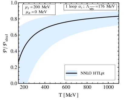
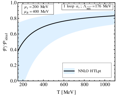
Figure 1: The pressure normalized to that of an ideal gas of massless particles as a function of $T$. Left figure is for $\mu_{I}=200$ Mev, $\mu_{B}=0$ and right figure is for $\mu_{I}=200$ MeV, $\mu_{B}=400$ MeV.

In Fig. 2, we show the normalized NNLO pressure of HTLpt as a function of $T$ for four different values of the isospin chemical potential $\mu_{I}$. We notice that the pressure is an increasing function of $\mu_{I}$ for fixed temperature and that the pressure curves converge at a temperature of approximately 800 MeV.

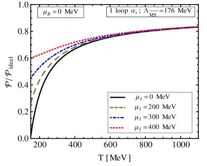
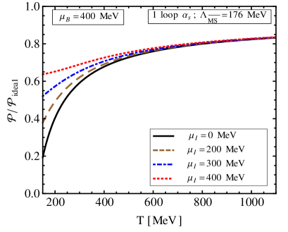
Figure 2: The pressure normalized to that of an ideal gas of massless particles as a function of $T$ for various values of the isospin chemical potential $\mu_{I}$ at $\mu_{B}=\mu_{S}=0$ (left) and $\mu_{B}=400$ MeV, $\mu_{S}=0$ (right). Here $\Lambda_{g}=2\pi T$ and $\Lambda_{q}=2\pi\sqrt{T^{2}+(\mu_{B}^{2}+2\mu_{I}^{2})/(3\pi^{2})}$ were used.

IV.3 Energy density

Once we know the pressure ${\cal P}$, we can calculate the energy density ${\cal E}$ by the Legendre transform

$${\cal E} = T{\partial{\cal P}\over\partial T}+\mu_{q}{\partial{\cal P}\over\partial\mu_{q}}-{\cal P}$$ (36)

$$= T{\partial{\cal P}\over\partial T}+\mu_{I}{\partial{\cal P}\over\partial\mu_{I}}-{\cal P}\;.$$

where we have used that $\mu_{I}={1\over 2}(\mu_{u}-\mu_{d})$ and $\mu_{s}=0$. In Fig. 3, we show the energy density as a function of the temperature for $\mu_{I}=0$ (left) and $\mu_{I}=200$ MeV (right). As in the case of the pressure, the energy density is an increasing function of $T$ and stays well below the ideal-gas value for all temperatures.

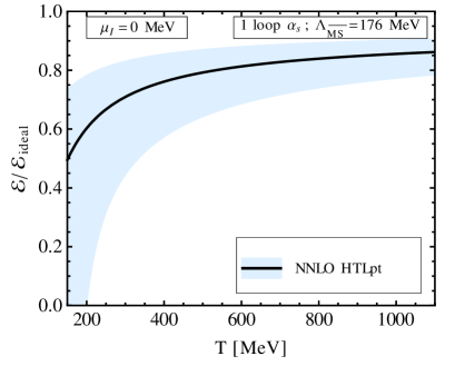
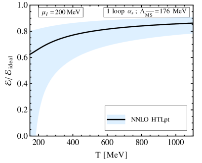
Figure 3: The energy density normalized to that of an ideal gas of massless particles as a function of $T$. Left figure is for $\mu_{I}=0$ and right figure is for $\mu_{I}=200$ MeV. $\mu_{B}=\mu_{S}=0$ in both plots.

In Fig. 4, we show the normalized energy density for four different values a of the isospin chemical potential $\mu_{I}$. For $\mu_{I}=0$ or $\mu_{I}=200$, the energy density is an increasing function of $T$. Note, however, that there is a minimum for the energy density for low temperatures and higher values of the isospin chemical potential. We would like to mention here that HTLpt probably cannot be trusted at these low temperatures with large chemical potential and one can not attribute any interesting physics to this nonmonotonic behavior.

Likewise, the curves converge at high temperatures, here already at approximately $T=600$ MeV.

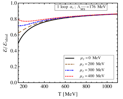
Figure 4: The energy density normalized to that of an ideal gas of massless particles as a function of $T$ for four different values of the isospin chemical potential and $\mu_{B}=\mu_{S}=0$. Here $\Lambda_{g}=2\pi T$ and $\Lambda_{q}=2\pi\sqrt{T^{2}+2\mu_{I}^{2}/(3\pi^{2})}$ were used.

IV.4 Trace anomaly

The trace anomaly or interaction measure ${\cal I}$ is defined by the difference

$${\cal I} = {\cal E}-3{\cal P}\;.$$ (37)

For an ideal gas of massless particles, the trace anomaly vanishes since ${\cal E}=3{\cal P}$. For massless particles and nonzero $g$, ${\cal I}$ is nonzero and is a measure of the interactions in the plasma. In Fig. 5, we show the interaction measure as a function of the temperature for two different values of the isospin chemical potential, $\mu_{I}=0$ (left) and $\mu_{I}=200$ MeV (right). The trace anomaly is a decreasing function of $T$ and it converges to zero for large values of $T$ due to asymptotic freedom.

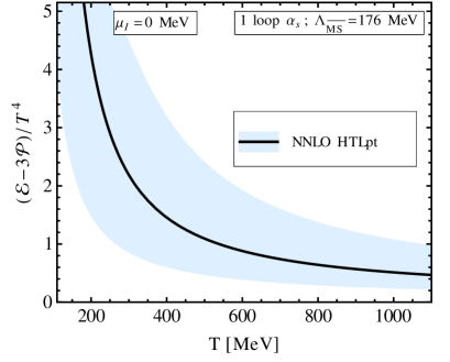
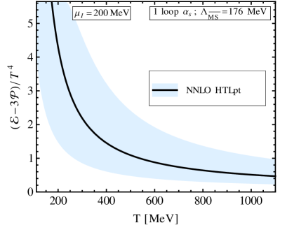
Figure 5: Trace anomaly divided by $T^{4}$ as a function of the temperature $T$. Left figure is for $\mu_{I}=0$ and right figure is for $\mu_{I}=200$ MeV. $\mu_{B}=\mu_{S}=0$ in both plots.

In Fig. 6, we show the normalized interaction measure as a function of the temperature $T$ for four different values of the isospin chemical potential $\mu_{I}$. As the figure demonstrates, the curves are essentially identical.

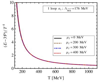
Figure 6: Trace anomaly divided by $T^{4}$ as a function of the temperature $T$ for four different values of the isospin chemical potential and $\mu_{B}=\mu_{S}=0$. Here $\Lambda_{g}=2\pi T$ and $\Lambda_{q}=2\pi\sqrt{T^{2}+2\mu_{I}^{2}/(3\pi^{2})}$ were used.

IV.5 Speed of sound

The speed of sound $c_{s}$ is defined by

$$c_{s}^{2} = {\partial{\cal P}\over\partial{\cal E}}\;.$$ (38)

In Fig. 7, we show the speed of sound squared $c_{s}^{2}$ for two different values of the isospin chemical potential, $\mu_{I}=0$ (left) and $\mu_{I}=200$ MeV (right). The horizontal dotted line is the ideal-gas value $c_{s}^{2}={1\over 3}$. As this figure demonstrates, the speed of sound is an increasing function of $T$.

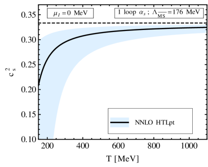
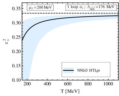
Figure 7: Speed of sound squared as a function of the temperature $T$. Left figure is for $\mu_{I}=0$ and right figure is for $\mu_{I}=200$ MeV. $\mu_{B}=\mu_{S}=0$ in both plots.

In Fig. 8, we show the speed of sound squared $c_{s}^{2}$ for four different values of the isospin chemical potential $\mu_{I}$. We notice that the speed of sound is an increasing function of $\mu_{I}$ for fixed $T$ and that the curves converge rather quickly, here at approximately $T=400$ MeV.

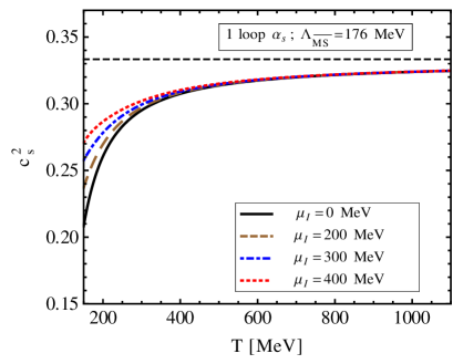
Figure 8: Speed of sound squared as a function of the temperature $T$ for different values of the isospin chemical potential $\mu_{I}$ and $\mu_{B}=\mu_{S}=0$. Here $\Lambda_{g}=2\pi T$ and $\Lambda_{q}=2\pi\sqrt{T^{2}+2\mu_{I}^{2}/(3\pi^{2})}$ were used.

IV.6 Susceptibilities

Using the thermodynamic potential given by Eq. (35), we can compute the quark-number susceptibilities. In the most general case, we have one quark chemical potential $\mu_{f}$ for each quark flavor $f$, which we can organize in an $N_{f}$-dimensional vector $\bm{\mu}=(\mu_{u},\mu_{d},\mu_{s},...,\mu_{N_{f}})$. The single quark susceptibilities are defined by

$$\chi_{ijk...}(T) = {\partial^{i+j+k+...}{\cal P}(T,{\bm{\mu}})\over\partial\mu_{u}^{i}\partial\mu_{d}^{j}\partial\mu_{s}^{k}...}\bigg{|}_{{\bm{\mu}}={\bm{\mu}_{0}}}\;,$$ (39)

where $\bm{\mu}_{0}$ is a configuration of quark chemical potentials. When computing the derivatives with respect to the chemical potential, we will use $\bm{\mu}_{0}=\bm{0}$. We treat $\Lambda_{q}$ as being a constant and only put the chemical potential dependence of $\Lambda_{q}$ in after the derivatives are taken. We have done this in order to more closely match the procedure used to compute the susceptibilities using resummed dimensional reduction vuorinen1 and to ensure that the susceptibilities vanish when $N_{f}=0$. In the following, we will use a shorthand notation for the quark susceptibilities by specifying derivatives by a string of quark flavors using superscript. For example, $\chi^{uu}_{2}=\chi_{200}$, $\chi^{ds}_{2}=\chi_{011}$, and $\chi^{uudd}_{4}=\chi_{220}$. For a three-flavor system with $(u,d,s)$ quarks with $\mu_{B}=\mu_{S}=0$ , the n’th-order isospin number susceptibility evaluated at $\mu_{I}=0$ is defined by

$$\chi^{I}_{n} \equiv {\partial^{n}{\cal P}\over\partial\mu_{I}^{n}}\bigg{|}_{\begin{subarray}{c}\hat{\mu}_{I}=0\end{subarray}}\;.$$ (40)

We can analytically express various order susceptibilities as

$$\chi^{I}_{2} = \frac{1}{48}T^{2}\left(32N_{c}-3d_{A}\hat{m}_{D}^{2}\hat{m}_{D}^{\prime\prime}\right)-\frac{d_{A}\alpha_{s}T^{2}}{96\pi}\Bigg{[}16(3-6\hat{m}_{D}+7\hat{m}_{D}^{3}\zeta(3))-\Bigg{\{}2(2c_{A}+N_{f})-24c_{A}\hat{m}_{D}$$

$$- \left(15c_{A}-36\gamma_{E}+66c_{A}\gamma_{E}+6N_{f}-72\log 2-36\ln\frac{\hat{\Lambda}}{2}+66c_{A}\ln\frac{\hat{\Lambda}}{2}\right)\hat{m}_{D}^{2}\Bigg{\}}\hat{m}_{D}^{\prime\prime}\Bigg{]}$$

$$+ \frac{d_{A}\alpha_{s}^{2}T^{2}}{144\pi^{2}}\Bigg{[}\frac{24(3+2c_{A})}{\hat{m}_{D}}+360-91c_{A}+105c_{F}+12c_{A}\gamma_{E}-146N_{f}+24\gamma_{E}N_{f}$$

$$+ (-504+144c_{A}+96c_{F}+168N_{f})\frac{\zeta^{\prime}(-1)}{\zeta(-1)}-(72+112c_{A}-48c_{F}+8N_{f})\log 2$$

$$- (132c_{A}-24N_{f})\log\frac{\hat{\Lambda}}{2}+288c_{A}\log\hat{m}_{D}-12\Big{(}36c_{F}+36\gamma_{E}-6N_{f}+72\log 2$$ (41)

$$- 6(11c_{A}-2N_{f})\log\frac{\hat{\Lambda}}{2}-21\zeta(3)-c_{A}(33+66\gamma_{E}+14\zeta(3))\Big{)}\hat{m}_{D}$$

$$- \Bigg{\{}\frac{(3+2c_{A})^{2}}{4\hat{m}_{D}^{2}}+\frac{6(3+2c_{A})}{\hat{m}_{D}}+\frac{3}{4}\Big{(}3c_{A}(9+14\gamma_{E}-16\log 2)-c_{A}^{2}(79-44\gamma_{E}+4\pi^{2}-44\log 2)$$

$$- 6(6c_{F}+6\gamma_{E}-N_{f}+12\log 2)+2(21c_{A}+22c_{A}^{2}-6N_{f})\ln\frac{\hat{\Lambda}}{2}\Big{)}\Bigg{\}}\hat{m}_{D}^{\prime}\Bigg{]}\;,$$

$$\chi^{I}_{4} = \frac{1}{\pi^{2}}\left(4N_{c}-\frac{d_{A}\hat{m}_{D}}{64}\left(6\hat{m}_{D}^{\prime\prime 2}+\hat{m}_{D}\hat{m}_{D}^{iv}\right)\right)-\frac{d_{A}\alpha_{s}}{384\pi^{3}}\Bigg{[}1152-5952\hat{m}_{D}^{3}\zeta(5)-\Big{(}576-2016\hat{m}_{D}^{2}\zeta(3)\Big{)}\hat{m}_{D}^{\prime\prime}$$ (42)

$$+\left\{72c_{A}-\left(216\gamma_{E}-90c_{A}-396c_{A}\gamma_{E}-36N_{f}+432\log 2+216\ln\frac{\hat{\Lambda}}{2}-396c_{A}\ln\frac{\hat{\Lambda}}{2}\right)\hat{m}_{D}\right\}\hat{m}_{D}^{\prime\prime 2}$$

$$-\left\{4c_{A}+2N_{f}-24c_{A}\hat{m}_{D}-\left(15c_{A}+6N_{f}-72\log 2-6(6-11c_{A})\left(\gamma_{E}+\ln\frac{\hat{\Lambda}}{2}\right)\right)\hat{m}_{D}^{2}\right\}\hat{m}_{D}^{iv}\Bigg{]}$$

$$+\frac{d_{A}\alpha_{s}^{2}}{24\pi^{4}}\Bigg{[}\frac{144}{\hat{m}_{D}}-36+21c_{F}(5+4\zeta(3))+72\gamma_{E}+2N_{f}\left(11+14\zeta(3)+12\ln\frac{\hat{\Lambda}}{2}\right)-576\log 2$$

$$-11c_{A}\left(17+12\gamma_{E}+24\log 2-7\zeta(3)+12\ln\frac{\hat{\Lambda}}{2}\right)+6\Big{(}168\zeta(3)-93\zeta(5)-62c_{A}\zeta(5)\Big{)}\hat{m}_{D}$$

$$+\Bigg{\{}-\frac{6(3+2cA)}{\hat{m}_{D}^{2}}+\frac{72c_{A}}{\hat{m}_{D}}+3(-36c_{F}-36\gamma_{E}+6N_{f}-72\log 2+6(11c_{A}-2N_{f})\ln\frac{\hat{\Lambda}}{2}$$

$$+21\zeta(3)+c_{A}(33+66\gamma_{E}+14\zeta(3))\Bigg{\}}\hat{m}_{D}^{\prime\prime}+\frac{(3+2c_{A})}{16\hat{m}_{D}^{3}}\Bigg{\{}(3+2c_{A})-12c_{A}\hat{m}_{D}\Bigg{\}}\hat{m}_{D}^{\prime\prime 2}$$

$$-\Bigg{\{}\frac{(3+2c_{A})^{2}}{96\hat{m}_{D}^{2}}-\frac{c_{A}(3+2c_{A})}{4\hat{m}_{D}}-\frac{1}{32}\Bigg{(}3c_{A}(9+14\gamma_{E}-16\log 2)+c_{A}^{2}(-79+44\gamma_{E}-4\pi^{2}+44\log 2)$$

$$-6(6c_{F}+6\gamma_{E}-N_{f}+12\log 2)+2(21c_{A}+22c_{A}^{2}-6N_{f})\ln\frac{\hat{\Lambda}}{2}\Bigg{)}\Bigg{\}}\hat{m}_{D}^{iv}\Bigg{]}\;,$$

where

$$\hat{m}_{D}^{\prime\prime} = \left.\frac{\partial^{2}\hat{m}_{D}}{\partial\hat{\mu}_{I}^{2}}\right|_{\begin{subarray}{c}\hat{\mu}_{I}=0\\ \hat{\mu}_{B}=0\end{subarray}}$$ (43)

$$= \frac{\alpha_{s}}{9\pi^{2}\hat{m}_{D}}\Bigg{[}36\pi+\alpha_{s}\Bigg{\{}6(11N_{c}-2N_{f})\ln\frac{\hat{\Lambda}}{2}-54c_{F}+N_{f}(6-12\gamma_{E}-24\log 2+7\zeta(3))$$

$$\hskip 56.9055pt+N_{c}(33+66\gamma_{E}+14\zeta(3))\Bigg{\}}\Bigg{]}\;,$$

$$\hat{m}_{D}^{iv} = \left.\frac{\partial^{4}\hat{m}_{D}}{\partial\hat{\mu}_{I}^{4}}\right|_{\begin{subarray}{c}\hat{\mu}_{I}=0\\ \hat{\mu}_{B}=0\end{subarray}}$$

$$= -\frac{\alpha_{s}^{2}}{54\pi^{4}\hat{m}_{D}^{3}}\Bigg{[}2\Bigg{\{}36\pi+\alpha_{s}\Big{(}6(11c_{A}-2N_{f})\ln\frac{\hat{\Lambda}}{2}-54c_{F}+N_{f}(6-12\gamma_{E}-24\log 2+7\zeta(3))$$

$$+c_{A}(33+66\gamma_{E}+14\zeta(3))\Big{)}\Bigg{\}}^{2}-\alpha_{s}\Bigg{\{}12\pi(2c_{A}+N_{f})+\alpha_{s}\Big{(}2(5+22\gamma_{E})c_{A}^{2}+3c_{A}(9+14\gamma_{E}-16\log 2)$$

$$-6(9c_{F}+N_{f}(-1+2\gamma_{E}+4\log 2))+2(21c_{A}+22c_{A}^{2}-6N_{f})\ln\frac{\hat{\Lambda}}{2}\Big{)}\Bigg{\}}\big{(}84N_{f}\zeta(3)-31(2c_{A}+N_{f})\zeta(5)\big{)}\Bigg{]}\;.$$

For a three-flavor system consisting of $(u,d,s)$ quarks, we can express the isospin susceptibilities in terms of the quark susceptibilities as

$$\chi^{I}_{2} = \left[\chi^{uu}_{2}+\chi^{dd}_{2}-2\chi^{ud}_{2}\right]\;,$$ (45)

$$\chi^{I}_{4} = \left[\chi^{uuuu}_{4}+\chi^{dddd}_{4}-4\chi^{uuud}_{4}-4\chi^{dddu}_{4}+6\chi^{uudd}_{4}\right]\;.$$ (46)

The isospin susceptibilities are expressed in terms of diagonal (same flavor on all indices) quark susceptibilities or off-diagonal (different flavor on some or all indices). In HTLpt, there are off-diagonal susceptibilities arising explicitly from some of the three-loop graphs 3loopqcd2 ; complete . There also potential off-diagonal contributions coming from all HTL terms since the mass parameter $m_{D}$ receives contributions from all quark flavors. However, these contributions vanish when we evaluate the susceptibilities at $\mu_{f}=0$. In this case, the HTLpt second and fourth-order isospin susceptibilities reduce to

$$\chi^{I}_{2} = 2\chi^{uu}_{2}\;,$$ (47)

$$\chi^{I}_{4} = \left[2\chi^{uuuu}_{4}+6\chi^{uudd}_{4}\right]\;.$$ (48)

In Fig. 9, we show the HTLpt predictions for the isospin second and fourth-order susceptibilities $\chi_{2}^{I}/T^{2}$ and $\chi_{4}^{I}$ as functions of $T$. The horizontal dotted lines are the corresponding isospin susceptibilities for an ideal gas, indicated by Stefan-Boltzmann limit. The central line for the second-order susceptibility is almost flat, while the central line for the and fourth-order susceptibility is slowly increasing.

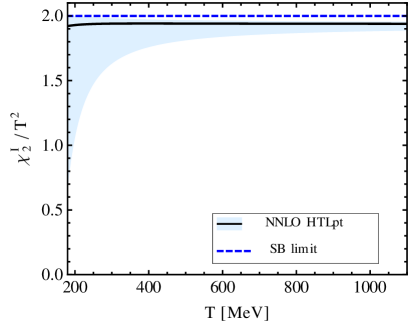
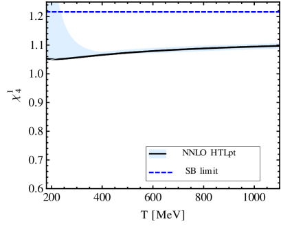
Figure 9: Second and fourth-order susceptibilities as functions of the temperature $T$ normalized to $T^{2}$ and one, respectively.

$\mu_{I}=\mu_{B}=\mu_{S}=0$ in both plots.

V Summary

In this paper, we presented results for a number of thermodynamic functions of QCD at finite temperature $T$ and finite isospin chemical potential $\mu_{I}$ using hard-thermal-loop perturbation theory. The pressure was also calculated at nonzero baryon chemical potential $\mu_{B}$. Our results were derived from the three-loop thermodynamic potential, which was computed in Ref. complete as a function of temperature and quark chemical potentials. Our final results depend on two renormalization scales $\Lambda_{g}$ and $\Lambda_{q}$ which are expected to be approximately $2\pi T$ and $2\pi\sqrt{T^{2}+(\mu_{B}^{2}+2\mu^{2}_{I})/(3\pi^{2})}$. In order to gauge the theoretical uncertainty associated with the scale choice, we varied both $\Lambda_{g}$ and $\Lambda_{q}$ by a factor of two (light-blue bands in some figures). We found that most quantities have a sizable scale variation and, at this moment in time, we do not have a method to reduce the size of the bands. A solution to this problem is suggested by the authors of Ref. kneur . In this approach, dubbed renormalization group optimized perturbation theory, the authors modify standard optimized perturbation theory or SPT. This is done by changing the added/subtraction mass term, including a finite vacuum term, and imposing renormalization group invariance on the pressure. In the case of $\phi^{4}$-theory, the result for the pressure up to two-loop order is very stable and with narrow bands under a scale variation. Note, however, that some quantities, e.g. $\chi_{4}^{I}$, have very small scale variation for temperatures $T\gtrsim$ 400 MeV and hence HTLpt provides testable predictions.

Given the relatively good agreement between lattice results and the predictions of NNLO HTLpt at zero and finite baryon chemical potential for $T\gtrsim 250$ MeV, we expect that the lattice results at finite $\mu_{I}$ should fall close to the central (black) lines predicted herein at high temperatures. We are looking forward to lattice measurements of QCD thermodynamics at finite $\mu_{I}$ and high temperatures (with $\mu_{B}=\mu_{S}=0$) in order to test the predictions made herein. Since the necessary lattice measurements can be done without Taylor expansion, they would provide a high-precision test of NNLO HTLpt.

References

- (1) K. Kajantie, M. Laine, K. Rummukainen and Y. Schroder, Phys. Rev. D 67, 105008 (2003).
- (2) A. Vuorinen, Phys. Rev. D 67, 074032 (2003).
- (3) A. Vuorinen, Phys. Rev. D 68, 054017 (2003).
- (4) A. Ipp, K. Kajantie, A. Rebhan, and A. Vuorinen, Phys. Rev. D74, 045016 (2006).
- (5) F. Karsch, A. Patkos and P. Petreczky, Phys. Lett. B 401, 69 (1997).
- (6) S. Chiku and T. Hatsuda, Phys. Rev. D 58, 076001 (1998).
- (7) J.O. Andersen, E. Braaten and M. Strickland, Phys. Rev. D 63, 105008 (2001).
- (8) J.O. Andersen and L. Kyllingstad, Phys. Rev. D 78, 076008 (2008).
- (9) V.I. Yukalov, Teor. Mat. Fiz. 26 403, (1976).
- (10) P.M. Stevenson, Phys. Rev. D 23, 2916 (1981).
- (11) A. Duncan and M. Moshe, Phys. Lett. B 215, 352 (1988).
- (12) A. Duncan and H.F. Jones, Phys. Rev. D 47, 2560 (1993).
- (13) A.N. Sisakian, I.L. Solovtsov, and O. Shevchenko, Int. J. Mod. Phys. A 9, 1929 (1994).
- (14) W. Janke and H. Kleinert, Phys. Rev. Lett. 75, 2787 (1995).
- (15) J. -L. Kneur and M.B. Pinto, Phys. Rev. Lett. 116, 031601 (2016). Phys.Rev. D 92, 116008 (2015).
- (16) J. O. Andersen, E. Braaten, and M. Strickland, Phys. Rev. Lett. 83, 2139 (1999).
- (17) N. Su., J. O. Andersen, and M. Strickland, Phys. Rev. Lett. 104, 122003 (2010).
- (18) J. O. Andersen, M. Strickland, and N. Su, JHEP 1008, 113 (2010).
- (19) J.O. Andersen, L.E. Leganger, M. Strickland and N. Su, Phys. Lett. B 696, 468 (2011).
- (20) J. O. Andersen, L. E. Leganger, M. Strickland and N. Su, JHEP 1108, 053 (2011).
- (21) J. O. Andersen, L. E. Leganger, M. Strickland and N. Su, Phys. Rev. D 84, 087703 (2011).
- (22) N. Haque, J. O. Andersen, M. G. Mustafa, M. Strickland, and N. Su, Phys. Rev. D 89, 061701 (2014).
- (23) N. Haque, A. Bandyopadhyay, J. O. Andersen, M. G. Mustafa, M. Strickland, and N. Su, JHEP 1405, 027 (2014).
- (24) P. Chakraborty, M. G. Mustafa, and M. H. Thoma, Eur. Phys. J. C. 23, 591 (2002).
- (25) P. Chakraborty, M. G. Mustafa, and M. H. Thoma, Phys. Rev. D 67, 114004 (2003).
- (26) P. Chakraborty, M. G. Mustafa, and M. H. Thoma, Phys. Rev. D 68, 085012 (2003).
- (27) N. Haque, M. G. Mustafa and M. H. Thoma, Phys. Rev. D 84, 054009 (2011).
- (28) N. Haque and M. G. Mustafa, Nucl. Phys. A 862-863, 271 (2011).
- (29) N. Haque and M. G. Mustafa, arXiv:1007.2076.
- (30) J.P. Blaizot, E. Iancu, and A. Rebhan, Eur. Phys. J. C 27, 433 (2003).
- (31) J.P. Blaizot, E. Iancu, and A. Rebhan Phys. Lett. B 523, 143 (2001).
- (32) J.P. Blaizot, E. Iancu, and A. Rebhan, Nucl. Phys. A 698, 404 (2002).
- (33) J.P. Blaizot, E. Iancu, and A. Rebhan, Phys. Rev. Lett. 83, 2906 (1999).
- (34) J.P. Blaizot, E. Iancu, and A. Rebhan, Phys. Lett. B 470, 181 (1999).
- (35) J.P. Blaizot, E. Iancu, and A. Rebhan, Phys. Rev. D 63, 065003 (2001).
- (36) E. Dagotto, F. Karsch, and A. Moreo, Phys. Lett. B 169, 421 (1986); E. Dagotto, A. Moreo, and U. Wolff, Phys. Rev. Lett. 57, 1292 (1986).
- (37) S. Hands, J.B. Kogut, M.-P. Lombardo, S. E. Morrison, Nucl. Phys. B 558, 327 (1999).
- (38) M. G. Alford, A. Kapustin, and F. Wilczek, Phys.Rev. D 59, 054502 (1999).
- (39) J. B. Kogut and D. K. Sinclair, Phys. Rev. D 66, 014508 (2002).
- (40) J. B. Kogut and D. K. Sinclair, Phys. Rev. D 66, 034505 (2002).
- (41) J. B. Kogut and D. K. Sinclair, Phys. Rev. D 70, 094501 (2004).
- (42) C. R. Allton, M. Doring, S. Ejiri, S. J. Hands, O. Kaczmarek, F. Karsch, E. Laermann, and K. Redlich, Phys. Rev. D 71, 054508 (2005).
- (43) S. Ejiri, F. Karsch, and K. Redlich, Phys. Lett. B 633, 275 (2006).
- (44) P. de Forcrand, M. A. Stephanov, and U. Wenger, PoS LAT2007, 237 (2007).
- (45) W. Detmold, K. Origonos, and Z. Shi, Phys. Rev. D 86, 05407 (2012).
- (46) G. Endrődi, Phys. Rev. D 90, 094501 (2014). forc
- (47) D. T. Son and M. A. Stephanov, Phys. Atom. Nucl. 64, 834 (2001).
- (48) S. Borsanyi, G. Endrodi, Z. Fodor, A. Jakovac, S. D. Katz, S. Krieg, C. Ratti and K. K. Szabo, JHEP 1011, 077 (2010).
- (49) S. Borsanyi, Z. Fodor, S. D. Katz, S. Krieg, C. Ratti and K. Szabo, JHEP 1201, 138 (2012)
- (50) S. Borsanyi, S. Durr, Z. Fodor, C. Hoelbling, S. D. Katz, S. Krieg, D. Nogradi and K. K. Szabo, B. C. Toth, and N. Trombitas, JHEP 1208, 126 (2012).
- (51) Sz. Borsányi, G. Endrődi, Z. Fodor, S.D. Katz, S. Krieg, C. Ratti and K.K. Szabó, JHEP 08, 053 (2012).
- (52) S. Borsanyi, Nucl. Phys. A904-905 2013, 270c (2013).
- (53) S. Borsanyi, Z. Fodor, S. D. Katz, S. Krieg, C. Ratti and K. K. Szabo, Phys. Rev. Lett. 111, 062005 (2013).
- (54) S. Sharma, Adv. High Energy Phys. 2013, 452978 (2013).
- (55) F. Karsch, B. -J. Schaefer, M. Wagner and J. Wambach, Phys. Lett. B 698, 256 (2011).
- (56) A. Bazavov, H. -T. Ding, P. Hegde, O. Kaczmarek, F. Karsch, E. Laermann, Y. Maezawa and S. Mukherjee et al., Phys. Rev. Lett. 111, 082301 (2013).
- (57) A. Bazavov, H. -T. Ding, P. Hegde, F. Karsch, C. Miao, S. Mukherjee, P. Petreczky and C. Schmidt, and A. Velytsky, Phys. Rev. D 88, 094021 (2013).
- (58) A. Bazavov, H. T. Ding, P. Hegde, O. Kaczmarek, F. Karsch, E. Laermann, S. Mukherjee and P. Petreczky et al., Phys. Rev. Lett. 109, 192302 (2012).
- (59) C. Bernard et al., Phys. Rev. D 71, 034504 (2005).
- (60) A. Bazavov, T. Bhattacharya, M. Cheng, N. H. Christ, C. DeTar, S. Ejiri, S. Gottlieb and R. Gupta et al., Phys. Rev. D 80, 014504 (2009).
- (61) A. Bazavov et al., Phys. Rev. D 86, 034509 (2012).
- (62) P. Petreczky, J. Phys. G 39, 093002 (2012).
- (63) HotQCD Collaboration (A. Bazavov (Iowa U.) et al.), Phys. Rev. D 90, 094503, (2014).
- (64) H.-T. Ding, F. Karsch, S. Mukherjee, Int. J. Mod. Phys. E 24, 1530007 (2015).
- (65) R. Bellwied, S. Borsanyi, Z. Fodor, S.D. Katz, A. Pasztor, C. Ratti, and K. K. Szabo, Phys. Rev. D 92, 114505 (2015).
- (66) H. -T. Ding, S. Mukherjee, H. Ohno, P. Petreczky, and H. -P. Schadler, Phys. Rev. D 92, 074043 (2015).
- (67) E. Braaten and R. D. Pisarski, Phys. Rev. D 45, R1827 (1992).
- (68) E. Braaten and A. Nieto, Phys. Rev. D 53, 3421 (1996).
- (69) D. J. Gross and F. Wilczek, Phys. Rev. Lett. 30, 1343 (1973).
- (70) H. D. Politzer, Phys. Rev. Lett. 30, 1346 (1973).
- (71) A. Bazavov, N. Brambilla, X. Garcia i Tormo, P. Petreczky, J. Soto and A. Vairo, Phys. Rev. D 86, 114031 (2012).