Superconvergence of Immersed Finite Element Methods for Interface Problems

Abstract

In this article, we study superconvergence properties of immersed finite element methods for the one dimensional elliptic interface problem. Due to low global regularity of the solution, classical superconvergence phenomenon for finite element methods disappears unless the discontinuity of the coefficient is resolved by partition. We show that immersed finite element solutions inherit all desired superconvergence properties from standard finite element methods without requiring the mesh to be aligned with the interface. In particular, on interface elements, superconvergence occurs at roots of generalized orthogonal polynomials that satisfy both orthogonality and interface jump conditions.

fourierlargesymbols147

1 Introduction

Immersed finite element (IFE) methods are a class of finite element methods (FEM) for solving differential equations with discontinuous coefficients, often known as interface problems. Unlike the classical FEM whose mesh is required to be aligned with the interface, IFE methods do not have such restriction. Consequently, IFE methods can use more structured, or even uniform meshes to solve interface problem regardless of interface location. This flexibility is advantageous for problems with complicated interfacial geometry [37] or for dynamic simulation involving a moving interface [22, 28, 29].

The main idea of IFE methods is to adapt approximating functions instead of meshes to fit the interface. On elements containing (part of) the interface, which we call interface elements, universal polynomials cannot approximate the solution accurately because of the low regularity of solution at the interface. A simple remedy is to construct piecewise polynomials as basis functions on interface elements in order to mimic the exact solution. The first IFE method was developed by Li [25] for solving the one-dimensional two-point boundary value problem. Piecewise linear shape functions were constructed on interface elements to incorporate the interface jump conditions. Following this idea, a family of quadratic IFE functions were introduced in [9]. Later in [1, 2], Adjerid and Lin extended the IFE approximation to arbitrary polynomial degree, and proved the optimal error estimates in the energy and the $L^{2}$-norms. In the past decade, IFE methods have also been extensively studied for a variety of interface problems in two dimension [19, 26, 27, 31, 32, 33] and three dimension [23, 37].

There have been many studies in the mathematical theories for IFE methods, for example [2, 17, 21, 25, 30]. Most of theoretical analysis focuses on error estimation in Sobolev $H^{1}$- and $L^{2}$- norms, but very few literature are concerned with the pointwise convergence. To the best of our knowledge, there is no systematic study on superconvergence phenomenon of IFE methods. Superconvergence theory for classical finite element methods [4, 18, 38] are invalid for IFE methods, unless the discontinuity of coefficient is resolved by the solution mesh.

Superconvergence phenomena of FEM were discussed as early as 1967 by Zienkiewicz and Cheung [45]. Later, Douglas and Dupont in [18] proved that the $p$-th order $C^{0}$ finite element method to the two-point boundary value problem converges with rate $O(h^{2p})$ at nodal points. Since then the superconvergence behavior of FEM has been studied intensively. We refer to [5, 6, 15, 24, 36, 38] for an incomplete list of references. In the mean time, there also has been considerable interest in studying superconvergence for other numerical methods, for example, spectral and spectral collocation methods [42, 43, 44], finite volume methods [8, 12, 14, 16, 40], discontinuous Galerkin and local discontinuous Galerkin methods [3, 10, 11, 13, 20, 39, 41].

In this article, we focus on the conforming $p$-th degree IFE methods for the prototypical one-dimensional elliptic interface problem. There are two major contributions in this article. First, we present a novel approach for developing IFE basis functions. The idea is completely different from classical approaches [1, 2], and the construction is based on the theory of orthogonal polynomials. Our new IFE bases accommodate interface jump conditions, and they satisfy certain orthogonality conditions which will be specified later. These basis functions can be explicitly constructed without solving linear systems. In an interface element, these IFE bases are either polynomials or piecewise polynomials, hence we call them generalized orthogonal polynomials.

Next, we analyze superconvergence properties of IFE methods. We will show that superconvergence phenomena occur at the roots of generalized orthogonal polynomials. To be more specific, the convergence rate of $p$-th degree IFE solutions is $O(h^{p+2})$ at nodal points. The accuracy at nodes can be improved to exact if the elliptic operator has only the diffusion term. The IFE solution converge to the exact solution with rate $O(h^{p+2})$ at the roots of generalized Lobatto polynomials, and the convergence rate of derivatives is escalated to $O(h^{p+1})$ at the roots of generalized Legendre polynomials. All the results can be viewed as an extension from the classic result for FEM [18].

The rest of the paper is organized as follows. In Section 2, we recall the IFE methods for interface problems and introduce some notations. In Section 3, we introduce the generalized orthogonal polynomials, based on which we present an explicit approach to construct IFE basis functions. In Section 4, we study the superconvergence properties of IFE methods for interface problems. In Section 5, we report some numerical results. A few concluding remarks are presented in Section 6.

2 Immersed Finite Element Methods

Let $\Omega=(a,b)$ be an open interval. Assume that $\alpha\in\Omega$ is an interface point such that $\Omega^{-}=(a,\alpha)$ and $\Omega^{+}=(\alpha,b)$. Consider the following one-dimensional elliptic interface problem

$$-(\beta u^{\prime})^{\prime}+\gamma u^{\prime}+cu=f,~{}~{}~{}x\in\Omega^{-}\cup\Omega^{+},$$ (2.1)

$$u(a)=u(b)=0.$$ (2.2)

The diffusion coefficient $\beta$ is assumed to have a finite jump across the interface $\alpha$. Without loss of generality, we assume that $\beta$ is a piecewise constant defined by

$$\beta(x)=\left\{\begin{array}[]{ll}\beta^{-},&\text{if}~{}x\in\Omega^{-},\\ \beta^{+},&\text{if}~{}x\in\Omega^{+},\end{array}\right.$$ (2.3)

where $\min\{\beta^{+},\beta^{-}\}>0$. The coefficients $\gamma$ and $c$ are assumed to be constants. At the interface $\alpha$, the solution is assumed to satisfy the interface jump conditions

$$\left[\!\left[u(\alpha)\right]\!\right]=0,~{}~{}~{}\left[\!\!\left[\beta u^{\prime}(\alpha)\right]\!\!\right]=0,$$ (2.4)

where $\left[\!\left[v(\alpha)\right]\!\right]:=v(\alpha^{+})-v(\alpha^{-})$. Denote the ratio of coefficient jump by $\rho=\frac{\beta_{\max}}{\beta_{\min}}$ where $\beta_{\max}=\max\{\beta^{+},\beta^{-}\}$, $\beta_{\min}=\min\{\beta^{+},\beta^{-}\}$

Throughout this article, we use standard notation of Sobolev spaces. We will also need to develop a few new spaces that characterize the interface problems. We define for $m\geq 1$ and $q\geq 1$ the Sobolev space

$$\tilde{W}_{\beta}^{m,q}(\Omega)=\Big{\{}v\in C(\Omega)\!\!\!\! : \!\!\!v|_{\Omega^{\pm}}\in W^{m,q}(\Omega^{\pm}),~{}v|_{\partial\Omega}=0,$$ (2.5)

$$\!\!\!\left[\!\!\left[\beta v^{(j)}(\alpha)\right]\!\!\right]=0,~{}j=1,2,\cdots,m\Big{\}},$$

equipped the norm and semi-norm

$$\|v\|_{m,q,\Omega}^{q}=\|v\|_{m,q,\Omega^{-}}^{q}+\|v\|_{m,q,\Omega^{+}}^{q},~{}~{}~{}|v|_{m,q,\Omega}^{q}=|v|_{m,q,\Omega^{-}}^{q}+|v|_{m,q,\Omega^{+}}^{q},$$

for $q<\infty$, and

$$\|v\|_{m,\infty,\Omega}=\max\{\|v\|_{m,\infty,\Omega^{-}},\|v\|_{m,\infty,\Omega^{+}}\},~{}~{}~{}|v|_{m,\infty,\Omega}=\max\{|v|_{m,\infty,\Omega^{-}},|v|_{m,\infty,\Omega^{+}}\}.$$

On a subset $\Lambda\subset\Omega$ that contains the interface point $\alpha$, we define

$$\|v\|_{m,q,\Lambda}^{q}=\|v\|_{m,q,\Lambda^{-}}^{q}+\|v\|_{m,q,\Lambda^{+}}^{q},\ \ |v|_{m,q,\Lambda}^{q}=|v|_{m,q,\Lambda^{-}}^{q}+|v|_{m,q,\Lambda^{+}}^{q},$$

where $\Lambda^{\pm}=\Lambda\cap\Omega^{\pm}$. If $\Lambda=\Omega$, we usually write $\|\cdot\|_{m,q}$ instead of $\|\cdot\|_{m,q,\Omega}$ for simplicity. In addition, if $q=2$, we simply write $\|\cdot\|_{m}$ instead of $\|\cdot\|_{m,q}$.

Next, we recall the main idea of the immersed finite element methods (IFEM) for interface problem (2.1) - (2.4). Consider the following interface-independent partition of $\Omega$:

$$a=x_{0}<x_{1}<\cdots<x_{k-1}\leq\alpha\leq x_{k}<\cdots<x_{N}=b.$$ (2.6)

Based on the partition (2.6), we define a mesh $\mathcal{T}_{h}=\{\tau_{i}\}_{i=1}^{N}$, where $\tau_{i}=(x_{i-1},x_{i})$. Denoted by $h_{i}=x_{i}-x_{i-1}$ the size of the element $\tau_{i}$, and by $h=\max\{h_{i},i=1,\cdots,N\}$ the mesh size of $\mathcal{T}_{h}$. Note that the interface $\alpha$ is located in the element $\tau_{k}$, which we call the interface element. The rest of elements $\tau_{i}$, $i\neq k$ are called noninterface elements. If the interface $\alpha$ coincides with the mesh point $x_{k-1}$ or $x_{k}$, then the partition (2.6) becomes interface-fitted; hence there is no difference between the IFEM and standard FEM.

Standard polynomials are used to as basis functions on all noninterface elements. To be more specific, we use the standard Lobatto polynomials as bases. The $p$-th degree FE space on the noninterface element $\tau_{i}$ is the standard polynomial space of degree $p$, denoted by ${\mathbb{P}}_{p}(\tau_{i})$. On the interface element $\tau_{k}$, we construct new IFE basis functions using the generalized Lobatto polynomials (will be defined in (3.8) - (3.12)). The corresponding $p$-th degree IFE space on $\tau_{k}$ is denoted by $\tilde{\mathbb{P}}_{p}(\tau_{k})$ shall be defined in (3.19) .

We define the $p$-th degree global IFE space on the mesh $\mathcal{T}_{h}$ by

$$S_{p}(\mathcal{T}_{h})=\{v\in H^{1}_{0}(\Omega):v|_{\tau_{i}}\in\mathbb{P}_{p}(\tau_{i}),\forall i\neq k;~{}v|_{\tau_{k}}\in\tilde{\mathbb{P}}_{p}(\tau_{k})\}$$

The IFEM for (2.1)-(2.4) is to find $u_{h}\in S_{p}(\mathcal{T}_{h})$ such that

$$(\beta u_{h}^{\prime},v_{h}^{\prime})+(\gamma u_{h}^{\prime},v_{h})+(cu_{h},v_{h})=(f,v_{h}),~{}~{}~{}\forall v_{h}\in S_{p}(\mathcal{T}_{h}),$$

where $(\cdot,\cdot)$ is the standard $L^{2}$ inner product on $(a,b)$.

3 Generalized Orthogonal Polynomials

In this section, we recall standard Legendre and Lobatto polynomials, and use them as basis functions on noninterface elements. Next, we construct the generalized orthogonal polynomials to be used as basis functions on interface elements.

3.1 Standard Orthogonal Polynomials

As usual, we construct basis functions on the reference interval $\tau=[-1,1]$, then map them to each physical element $\tau_{i}$ by appropriate affine mapping. Let $P_{n}(\xi)$ be the Legendre polynomial of degree $n$ on $\tau$ defined by

$$P_{n}(\xi)=\frac{1}{2^{n}n!}\frac{d^{n}}{d\xi^{n}}\big{[}(\xi^{2}-1)^{n}\big{]}$$

Legendre polynomials satisfy the following orthogonality

$$\int_{-1}^{1}P_{m}(\xi)P_{n}(\xi)d\xi=\frac{2}{2n+1}\delta_{mn}.$$ (3.1)

Define $\{\psi_{n}\}$ to be the family of Lobatto polynomials on $\tau=[-1,1]$,

$$\psi_{0}(\xi)=\frac{1-\xi}{2},~{}~{}~{}\psi_{1}(\xi)=\frac{1+\xi}{2},~{}~{}~{}\psi_{n}(\xi)=\int_{-1}^{\xi}P_{n-1}(t)dt,~{}~{}~{}n\geq 2.$$ (3.2)

3.2 Generalized Orthogonal Polynomials

On the interface element $\tau_{k}$ containing $\alpha$, we construct a sequence of polynomials satisfying both orthogonality and interface jump conditions. Again, we map $\tau_{k}$ to the reference interval $\tau=[-1,1]$ containing the reference interface point $\hat{\alpha}$. Let $\hat{\beta}(\xi)=\beta(x)$ such that $\hat{\beta}(\xi)=\beta^{-}$ on $\tau^{-}=(-1,\hat{\alpha})$ and $\hat{\beta}(\xi)=\beta^{+}$ on $\tau^{+}=(\hat{\alpha},1)$.

Define a sequence of orthogonal polynomials $\{L_{n}\}$ with the weight function $w(\xi)=\frac{1}{\hat{\beta}(\xi)}$, i.e.,

$$(L_{n},L_{m})_{w}:=\int_{-1}^{1}w(\xi)L_{n}(\xi)L_{m}(\xi)d\xi=c_{n}\delta_{mn},$$ (3.3)

where $c_{n}=\|L_{n}\|_{w}^{2}=(L_{n},L_{n})_{w}$. If we require $\{L_{n}\}$ to be monic polynomials, then they can be uniquely constructed via the following three-term recurrence formula ([35], Theorem 3.1):

Remark 3.1.

Let $\{{L}_{n}\}$ be the family of monic orthogonal polynomials satisfying (3.3). Then $\{{L}_{n}\}$ can be constructed as follows

$${L}_{0}(\xi)=1,~{}~{}~{}{L}_{1}(\xi)=\xi-a_{0},~{}~{}~{}$$ (3.4)

$${L}_{n+1}(\xi)=(\xi-a_{n}){L}_{n}(\xi)-b_{n}{L}_{n-1}(\xi),~{}~{}n\geq 1,$$ (3.5)

where

$$a_{n} = \frac{(\xi{L}_{n},{L}_{n})_{w}}{({L}_{n},{L}_{n})_{w}},~{}~{}~{}n\geq 0$$

$$b_{n} = \frac{({L}_{n},{L}_{n})_{w}}{({L}_{n-1},{L}_{n-1})_{w}},~{}~{}~{}n\geq 1.$$

The polynomials $\{L_{n}\}$ are generalized from standard Legendre polynomials $\{P_{n}\}$ by allowing the weight function to be discontinuous. Hence, we call $\{L_{n}\}$ the generalized Legendre polynomials.

Next, we define a sequence of piecewise polynomial $\{\phi_{n}\}$ in a similar manner as (3.2)

$$\phi_{0}(\xi) = \left\{\begin{array}[]{ll}\frac{(1-\hat{\alpha})\beta^{-}+(\hat{\alpha}-\xi)\beta^{+}}{(1-\hat{\alpha})\beta^{-}+(1+\hat{\alpha})\beta^{+}},&\text{in}~{}\tau^{-},\vspace{1mm}\\ \frac{(1-\xi)\beta^{-}}{(1-\hat{\alpha})\beta^{-}+(1+\hat{\alpha})\beta^{+}},&\text{in}~{}\tau^{+}.\end{array}\right.$$ (3.8)

$$\phi_{1}(\xi) = \left\{\begin{array}[]{ll}\frac{(1+\xi)\beta^{+}}{(1-\hat{\alpha})\beta^{-}+(1+\hat{\alpha})\beta^{+}},&\text{in}~{}\tau^{-},\vspace{1mm}\\ \frac{(\xi-\hat{\alpha})\beta^{-}+(1+\hat{\alpha})\beta^{+}}{(1-\hat{\alpha})\beta^{-}+(1+\hat{\alpha})\beta^{+}},&\text{in}~{}\tau^{+}.\end{array}\right.$$ (3.11)

$$\phi_{n}(\xi) = \int_{-1}^{\xi}w(t)L_{n-1}(t)dt,~{}~{}~{}n=2,3,\cdots$$ (3.12)

Note that $\phi_{0}$ and $\phi_{1}$ are constructed to fulfill nodal value conditions

$$\phi_{0}(-1)=1,~{}~{}\phi_{0}(1)=0,~{}~{}\phi_{1}(-1)=0,~{}~{}\phi_{1}(1)=1.$$

and the interface jump condition (2.4). In fact, $\phi_{0}$ and $\phi_{1}$ are piecewise linear polynomials, and they are exactly the two Lagrange type IFE nodal basis functions (see [2, 25]).

Theorem 3.1.

$\{\phi_{n}\}$ is a sequence of piecewise polynomials and satisfy

• the interface jump conditions

  $$\left[\!\left[\phi_{n}(\hat{\alpha})\right]\!\right]=0,~{}~{}~{}~{}\left[\!\!\left[\hat{\beta}\phi_{n}^{\prime}(\hat{\alpha})\right]\!\!\right]=0,~{}~{}~{}\forall n\geq 0,$$ (3.13)

• the weighted orthogonality condition

  $$\langle\phi_{m},\phi_{n}\rangle_{\hat{\beta}}:=\int_{-1}^{1}\hat{\beta}(\xi)\phi_{m}^{\prime}(\xi)\phi_{n}^{\prime}(\xi)d\xi=\tilde{c}_{n}\delta_{mn},~{}~{}~{}\forall m,n\geq 1,$$ (3.14)

  where $\tilde{c}_{n}$ is some nonzero constant.

Proof.

We first prove the interface jump conditions (3.13). It is true for $\phi_{0}$ and $\phi_{1}$ by direct verification using (3.8) and (3.11). For $n\geq 2$, we note that $\phi_{n}$ is continuous because it is defined through the integral (3.12). Moreover, since $\{L_{n}\}$ is a sequence of polynomials, then

$$\left[\!\!\left[\hat{\beta}\phi_{n}^{\prime}(\hat{\alpha})\right]\!\!\right]=\beta^{+}\phi_{n}^{\prime}(\hat{\alpha}+)-\beta^{-}\phi_{n}^{\prime}(\hat{\alpha}-)=L_{n-1}(\hat{\alpha}+)-L_{n-1}(\hat{\alpha}-)=0.$$

The orthogonality (3.14) follows from (3.3) and (3.12), i.e.,

$$\langle\phi_{m},\phi_{n}\rangle_{\hat{\beta}}=(L_{m-1},L_{n-1})_{w}=c_{n-1}\delta_{m-1,n-1}=\tilde{c}_{n}\delta_{mn}.$$

∎

The piecewise polynomials $\{\phi_{n}\}$ are generalized from standard Lobatto polynomials $\{\psi_{n}\}$ defined in (3.2). The construction (3.12) uses piecewise constant weight function $w(\xi)=\frac{1}{\hat{\beta}(\xi)}$ instead of a universal constant one. We call $\{\phi_{n}\}$ the generalized Lobatto polynomials.

The generalized Lobatto polynomials $\{\phi_{n}\}$ form a sequence of IFE basis functions satisfying both interface jump conditions and orthogonal conditions. In Figure 1, we plot a few generalized Legendre polynomials $L_{n}$ and generalized Lobatto polynomials $\phi_{n}$ for the configuration of $\hat{\alpha}=0.15$ and $\hat{\beta}=\{1,5\}$. In Figure 2, we plot the generalized polynomials for multiple (two) interface points $\hat{\alpha}=-0.15$ and $0.4$. The coefficient $\hat{\beta}$ has three pieces in this case, i.e., $\hat{\beta}=\{1,5,3\}$.

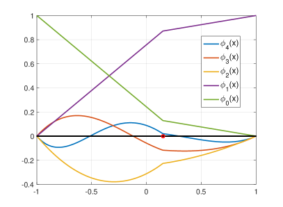
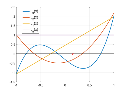
Figure 1: Generalized Lobatto (left) and Legendre (right) polynomials with one interface point

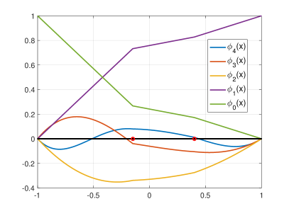
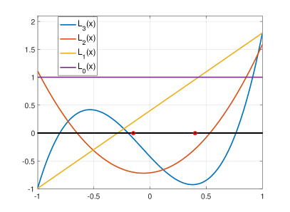
Figure 2: Generalized Lobatto (left) and Legendre (right) polynomials with two interface points

Remark 3.2.

The generalized Lobatto polynomials $\{\phi_{n}\}$ are identical (up to a multiple constant) to IFE basis functions introduced in [1]. However, the construction in this article is more explicit and does not require solving a linear system. This procedure is more advantageous when there are multiple discontinuities in an interval.

Remark 3.3.

In the construction procedure of $\phi_{n}$, we did not impose the extended interface jump conditions [1]:

$$\left[\!\!\left[\hat{\beta}\phi_{n}^{(j)}(\hat{\alpha})\right]\!\!\right]=0,~{}~{}~{}~{}\forall~{}j=2,3,\cdots,n.$$ (3.15)

However, it can be easily verified that all the generalized Lobatto polynomials $\{\phi_{n}\}$ satisfy (3.15) automatically.

We can obtain the local FE basis functions $\psi_{i,n}$ on each noninterface element $\tau_{i}$ and the IFE basic functions $\phi_{k,n}$ on the interface element $\tau_{k}$ by the following affine mappings,

$$\psi_{i,n}(x):=\psi_{n}(\xi)=\psi_{n}\left(\frac{2x-x_{i-1}-x_{i}}{h_{i}}\right),~{}~{}~{}~{}n\geq 0.$$ (3.16)

$$\phi_{k,n}(x):=\phi_{n}(\xi)=\phi_{n}\left(\frac{2x-x_{k-1}-x_{k}}{h_{k}}\right),~{}~{}~{}~{}n\geq 0.$$ (3.17)

Then the $p$-th degree local FE space $\mathbb{P}_{p}(\tau_{i})$ on noninterface elements $\tau_{i}$, $i\neq k$, and IFE space $\tilde{\mathbb{P}}_{p}(\tau_{k})$ on interface element $\tau_{k}$ are defined by

$$\mathbb{P}_{p}(\tau_{i})=\text{span}\{\psi_{i,n}:n=0,1,\cdots,p\}.$$ (3.18)

$$\tilde{\mathbb{P}}_{p}(\tau_{k})=\text{span}\{\phi_{k,n}:n=0,1,\cdots,p\}.$$ (3.19)

Finally, the $p$-th degree global IFE space is defined by

$$S_{p}(\mathcal{T}_{h}):=\{v\in H_{0}^{1}(\Omega):v|_{\tau_{i}}\in\mathbb{P}_{p}(\tau_{i}),~{}i\neq k,~{}\text{and}~{}v|_{\tau_{k}}\in\tilde{\mathbb{P}}_{p}(\tau_{k})\}.$$ (3.20)

The IFEM for the interface problem (2.1) - (2.4) is: find $u_{h}\in S_{p}(\mathcal{T}_{h})$ such that

$$a(u_{h},v_{h}):=(\beta u_{h}^{\prime},v_{h}^{\prime})+(\gamma u_{h}^{\prime},v_{h})+(cu_{h},v_{h})=(f,v_{h}),~{}~{}~{}~{}\forall v_{h}\in S_{p}(\mathcal{T}_{h}).$$ (3.21)

3.3 Properties of Generalized Orthogonal Polynomials

In this subsection, we investigate some fundamental properties of the generalized orthogonal polynomials.

First, it is interesting to know the number and distribution of zeros for the generalized Lobatto polynomials and generalized Legendre polynomials in the interval $[-1,1]$. To prove our main result, we need the following lemma.

Lemma 3.1.

(Generalized Rolle’s theorem) Assume that the function $f$ is real-valued and continuous on a closed interval $[a,b]$ with $f(a)=f(b)$. If for every $x$ in the open interval $(a,b)$, both of one side limits

$$f^{\prime}(x+)=\lim_{h\to 0^{+}}\frac{f(x+h)-f(x)}{h},~{}~{}~{}~{}f^{\prime}(x-)=\lim_{h\to 0^{-}}\frac{f(x+h)-f(x)}{h}$$

exist, then there is some number $c$ in the open interval $(a,b)$ such that one of the two limits $f^{\prime}(c+)$ and $f^{\prime}(c-)$ is $\geq 0$ and the other is $\leq 0$.

The above lemma generalizes the Rolle’s theorem to functions that are continuous on $[a,b]$, but not necessarily differentiable at all interior points of $(a,b)$. The proof is straightforward and similar to the standard Rolle’s theorem; hence we omit it in this article.

Theorem 3.2.

The generalized Legendre polynomials $\{L_{n}\}$ and generalized Lobatto polynomials $\{\phi_{n}\}$ have the same numbers of roots as the standard Legendre polynomials $\{P_{n}\}$ and Lobatto polynomials $\{\psi_{n}\}$, respectively, i.e.,

1. For $n\geq 1$, $L_{n}$ has $n$ simple roots in the open interval $(-1,1)$.

2. For $n\geq 1$, $\phi_{n+1}(\pm 1)=0$, and $\phi_{n+1}$ has $n-1$ simple “roots” in the open interval $(-1,1)$, i.e., the piecewise polynomial $\phi_{n+1}(\xi)$ crosses the $\xi$-axis $n-1$ times in $(-1,1)$.

Proof.

Note that $\{L_{n}\}$ is a family of orthogonal polynomials on $[-1,1]$. The weight function $w(\xi)=\hat{\beta}(\xi)^{-1}$ is positive and is a Lebesgue integrable function. Hence, the polynomial $L_{n}$ has $n$ simple roots in $(-1,1)$.

For the generalized Lobatto polynomial $\phi_{n+1}$, by its definition (3.11), it is obvious that $\phi_{n+1}(-1)=0$. The orthogonality condition (3.3) yields

$$\phi_{n+1}(1)=\int_{-1}^{1}w(\xi){L}_{n}(\xi)d\xi=\int_{-1}^{1}w(\xi){L}_{n}(\xi){L}_{0}(\xi)d\xi=0.$$

In the remaining of the proof, we will show that $\phi_{n+1}$ has exactly $n-1$ roots in the open interval $(-1,1)$. By (3.13) and (3.14), we have for $m\leq n$,

$$\int_{-1}^{1}\hat{\beta}\phi_{n+1}^{\prime}(\xi)\phi_{m}^{\prime}(\xi)d\xi = -\int_{-1}^{1}\phi_{n+1}(\xi)(\hat{\beta}\phi_{m}^{\prime})^{\prime}(\xi)d\xi$$

$$= -\int_{-1}^{1}\phi_{n+1}(\xi)L_{m-1}^{\prime}(\xi)d\xi=0.$$

Since $L_{m-1}^{\prime}\in\mathbb{P}_{m-2}(\tau)$, then

$$\int_{-1}^{1}\phi_{n+1}(\xi)v(\xi)d\xi=0,~{}~{}~{}\forall\ v\in\mathbb{P}_{n-2}(\tau).$$ (3.22)

In particular, choosing $v=1$ we have

$$\int_{-1}^{1}\phi_{n+1}(\xi)d\xi=0.$$

Since $\phi_{n+1}$ is continuous, and its average is zero over $(-1,1)$, therefore it must change signs at least once in $(-1,1)$. Let $\xi_{1}$, $\xi_{2}$, $\cdots$, $\xi_{k}$ be all points in $(-1,1)$ at which $\phi_{n+1}$ changes signs. We will show that $k=n-1$ by contradiction.

Suppose $k<n-1$. We choose $v(\xi)=(\xi-\xi_{1})(\xi-\xi_{2})\cdots(\xi-\xi_{k})\in\mathbb{P}_{n-2}(\tau)$ so that $\phi_{n+1}(\xi)v(\xi)$ does not change signs. The orthogonality (3.22) yields

$$\int_{-1}^{1}\phi_{n+1}(\xi)v(\xi)d\xi=0.$$ (3.23)

This contradicts (3.23).

Suppose $k>n-1$. Without loss of generality, we assume $-1<\xi_{1}<\cdots<\xi_{k}<1$ partitions $[-1,1]$ into $k+1$ subintervals, and $\hat{\alpha}\in(\xi_{i},\xi_{i+1})$. On all $k$ noninterface subintervals, applying standard Rolle’s theorem, we conclude that the derivative of $\phi_{n+1}(\xi)$ has at least one zero in each of these $k$ noninterface intervals. Hence, the weighted derivative $L_{n}(\xi)=\hat{\beta}\phi_{n+1}^{\prime}(\xi)$ has at least $k$ zeros on noninterface intervals.

On the interface subinterval $(\xi_{i},\xi_{i+1})$, $\phi_{n+1}$ is not differentiable at the interior point $\hat{\alpha}$, then by the generalized Rolle’s theorem (Lemma 3.1), there exists a point $c$ such that one of $\phi_{n+1}^{\prime}(c-)$ and $\phi_{n+1}^{\prime}(c+)$ is non-negative, and the other is non-positive. It can be directly verified that

$$L_{n}(c-)=\hat{\beta}(c-)\phi_{n+1}^{\prime}(c-),~{}~{}~{}~{}~{}L_{n}(c+)=\hat{\beta}(c+)\phi_{n+1}^{\prime}(c+)$$

are also one of each, because $\hat{\beta}$ is strictly positive. Also, $L_{n}$ is a polynomial, thus continuous everywhere including at $c$. Hence, $L_{n}(c)=0$. That is, the polynomial $L_{n}$ has a zero in $(\xi_{i},\xi_{i+1})$, which means $L_{n}(\xi)$ has at least $k+1(>n)$ zeros on $(-1,1)$. This contradicts the first part of the theorem.

In conclusion, $\phi_{n+1}$ has exactly $n-1$ roots on the open interval $(-1,1)$. ∎

Next we show the consistency of the generalized orthogonal polynomials with standard orthogonal polynomials.

Lemma 3.2.

If the interface coincides with the boundary i.e., $\hat{\alpha}=\pm 1$, or if there is no jump of coefficient, i.e., $\beta^{+}=\beta^{-}$, then $\{\phi_{n}\}$ and $\{L_{n}\}$ become standard Lobatto polynomial $\{\psi_{n}\}$ and Legendre polynomials $\{P_{n}\}$, respectively, up to a multiple constant.

Proof.

Suppose $\hat{\alpha}=-1$. The weight function $w(\xi)=\frac{1}{\beta^{+}}$ becomes a constant. By the recurrence formula (3.5), it is easy to see that ${L}_{n}=c_{n}{P}_{n}$, where $c_{n}$ is a constant. By (3.12) we have

$$\phi_{n}(\xi)=\int_{-1}^{\xi}\frac{1}{\beta^{+}}L_{n-1}(s)ds=\frac{1}{\beta^{+}}c_{n-1}\int_{-1}^{\xi}{P}_{n-1}(s)ds=\frac{1}{\beta^{+}}c_{n-1}\psi_{n}(\xi),$$

for some constant $c_{n-1}$.

When $\hat{\alpha}=1$, the argument is similar. When $\beta^{+}=\beta^{-}$, the weight function $w(\xi)=\frac{1}{\beta^{-}}$ becomes a constant. The corresponding result can be obtained following a similar argument as above. ∎

We define a class of differential operators $D_{x}^{j}$ and integral operators $D_{x}^{-j}$, $j\geq 1$:

$$(D_{x}^{1}v)\big{|}_{\tau_{i}}=(D_{x}v)\big{|}_{\tau_{i}}=v^{\prime}(x),~{}~{}(D_{x}^{j}v)\big{|}_{\tau_{i}}=D_{x}(D_{x}^{j-1}v)\big{|}_{\tau_{i}}$$ (3.24)

and $D_{x}^{-j}:\tilde{W}_{\beta}^{m,q}(\Omega)\rightarrow\tilde{W}_{\beta}^{m,q}(\Omega),j\geq 1$ by

$$(D_{x}^{-1}v)\big{|}_{\tau_{i}}=\int_{x_{i-1}}^{x}v(x)dx,\ \ (D_{x}^{-j}v)\big{|}_{\tau_{i}}=\int_{x_{i-1}}^{x}D_{x}^{-(j-1)}v(x)dx,\ \ j\geq 2.$$ (3.25)

Next we prove an important inverse inequality for generalized polynomials.

Lemma 3.3.

(Inverse Inequality) There exists a constant $C$, depending only on the polynomial degree $p$ such that

$$|v|_{l,q,\tau_{k}}\leq C\rho h^{m-l+\frac{1}{q}-\frac{1}{r}}|v|_{m,r,\tau_{k}},~{}~{}~{}\forall v\in\tilde{\mathbb{P}}_{p}(\tau_{k}),$$ (3.26)

where $1\leq q\leq\infty$, $1\leq r\leq\infty$, $0\leq m\leq l$, and $\rho=\frac{\beta_{max}}{\beta_{min}}$.

Proof.

First we consider $q<\infty$, and $r<\infty$.

$$|v|_{l,q,\tau_{k}}^{q} = \int_{\tau_{k}}|D_{x}^{l}v|^{q}dx$$ (3.27)

$$= \int_{\tau_{k}^{+}}\frac{1}{(\beta^{+})^{q}}|D_{x}^{l-1}(\beta^{+}v^{\prime})|^{q}dx+\int_{\tau_{k}^{-}}\frac{1}{(\beta^{-})^{q}}|D_{x}^{l-1}(\beta^{-}v^{\prime})|^{q}dx$$

$$\leq \frac{1}{(\beta_{min})^{q}}\int_{\tau_{k}}|D_{x}^{l-1}(\beta v^{\prime})|^{q}dx$$

$$= \frac{1}{(\beta_{min})^{q}}|\beta v^{\prime}|_{l-1,q,\tau_{k}}^{q}$$

Note that $\beta v^{\prime}$ is a polynomial for all $v\in\tilde{\mathbb{P}}_{p}(\tau_{k})$. In fact, $\beta v^{\prime}\in{\mathbb{P}}_{p-1}(\tau_{k})$. Standard inverse inequality [7] applied to $\beta v^{\prime}$ yields

$$|\beta v^{\prime}|_{l-1,q,\tau_{k}}\leq Ch^{m-l+\frac{1}{q}-\frac{1}{r}}|\beta v^{\prime}|_{m-1,r,\tau_{k}}$$ (3.28)

On the other hand,

$$|\beta v^{\prime}|_{m-1,r,\tau_{k}}^{r} = \int_{\tau_{k}}|D_{x}^{m-1}(\beta v^{\prime})|^{r}dx$$ (3.29)

$$= \int_{\tau_{k}^{+}}(\beta^{+})^{r}|D_{x}^{m}v|^{r}dx+\int_{\tau_{k}^{-}}(\beta^{-})^{r}|D_{x}^{m}v|^{r}dx$$

$$\leq (\beta_{max})^{r}\int_{\tau_{k}}|D_{x}^{m}v|^{r}dx$$

$$= (\beta_{max})^{r}|v|_{m,r,\tau_{k}}^{r}$$

Combining (3.27), (3.28), and (3.29) we have

$$|v|_{l,q,\tau_{k}}\leq C\rho h^{m-l+\frac{1}{q}-\frac{1}{r}}|v|_{m,r,\tau_{k}}$$ (3.30)

If $q=\infty$ (or $r=\infty$), we have

$$|v|_{l,\infty,\tau_{k}}=\lim_{q\to\infty}|v|_{l,q,\tau_{k}}~{}~{}~{}\forall v\in\tilde{\mathbb{P}}_{p}(\tau_{k}).$$

Thus, the estimate (3.30) holds true.

∎

4 Superconvergence Analysis

In this section, we analyze the superconvergence property for the IFE method (3.21). We first analyze the convergence estimates for interpolation. Then we discuss the superconvergence analysis for diffusion (only) interface problems i.e., $\gamma=c=0$ in (2.1). Finally, we consider the general elliptic interface problems, i.e., $\gamma\neq 0$, and $c\neq 0$.

4.1 IFE Interpolation

We consider the IFE interpolation using generalized Lobatto polynomials. For any $u\in\tilde{W}_{\beta}^{m,q}(\Omega),m\geq 1$, we have the following Lobatto expansion of $u$ on noninterface elements $\tau_{i}$

$$u(x)|_{\tau_{i}}=\sum_{n=0}^{\infty}u_{i,n}\psi_{i,n}(x),~{}~{}~{}i\neq k$$ (4.1)

where

$$u_{i,0}=u(x_{i-1}),\ \ u_{i,1}=u(x_{i}),\ \ u_{i,n}=\dfrac{\displaystyle\int_{\tau_{i}}u^{\prime}(x)\psi_{i,n}^{\prime}(x)dx}{\displaystyle\int_{\tau_{i}}\psi_{i,n}^{\prime}(x)\psi_{i,n}^{\prime}(x)dx},\ \ n\geq 2.$$ (4.2)

On the interface element $\tau_{k}$, since the flux $\beta u^{\prime}$ is continuous, then it can be expanded by generalized Legendre polynomials $\{L_{k,n}\}$

$$\beta u^{\prime}(x)=\sum_{n=0}^{\infty}u_{k,n}L_{k,n}(x){.}$$

Dividing by $\beta$ and then integrating on both sides yield the expansion for $u$

$$u(x)|_{\tau_{k}}=\sum_{n=0}^{\infty}u_{k,n}\int_{x_{k-1}}^{x}\frac{1}{\beta(t)}L_{k,n}(t)dt=\sum_{n=0}^{\infty}u_{k,n}\phi_{k,n}(x).$$ (4.3)

By the orthogonality (3.14) and the properties of generized Lobatto polynomials in Theorem 3.2, we have

$$u_{k,0}=u(x_{k-1}),\ \ u_{k,1}=u(x_{k}),\ \ u_{k,n}=\frac{\langle u,\phi_{k,n}\rangle_{\tau_{k}}}{\langle\phi_{k,n},\phi_{k,n}\rangle_{\tau_{k}}},~{}~{}~{}n\geq 2,$$ (4.4)

where

$$\langle u,v\rangle_{\tau_{k}}=\int_{x_{k-1}}^{x_{k}}\beta u^{\prime}(x)v^{\prime}(x)dx,~{}~{}~{}~{}\forall\ u,v\in\tilde{W}_{\beta}^{m,q}(\Omega).$$

Using the (generalized) Lobatto expansions (4.1) and (4.3) on noninterface and interface elements, we define the IFE interpolation $\mathcal{I}_{h}:\tilde{W}_{\beta}^{m,q}(\Omega)\to S_{p}{(\mathcal{T}_{h})}$ as follows

$$(\mathcal{I}_{h}u)|_{\tau_{i}}=\left\{\begin{array}[]{ll}\sum\limits_{n=0}^{p}u_{i,n}\psi_{i,n}(x),&\text{if}~{}i\neq k\vspace{1mm}\\ \sum\limits_{n=0}^{p}u_{i,n}\phi_{i,n}(x),&\text{if}~{}i=k.\end{array}\right.$$ (4.5)

Lemma 4.1.

There holds for all $j\leq n-2$

$$D_{x}^{-j}\phi_{k,n}(x_{k-1})=D_{x}^{-j}\phi_{k,n}(x_{k})=0$$ (4.6)

where $D_{x}^{-j}$ is the integral operator defined in (3.25).

Proof.

Note from (3.22) and Theorem 3.2 that

$$\phi_{k,n}(x_{k-1})=\phi_{k,n}(x_{k})=0,\ \ \ \int_{x_{k-1}}^{x_{k}}\phi_{k,n}(x)v(x)dx=0,\ \ \forall\ v\in\mathbb{P}_{n-3}(\tau_{k}).$$ (4.7)

Choosing $v=1$ in the above equation, we immediately obtain

$$D_{x}^{-1}\phi_{k,n}(x_{k})=\int_{x_{k-1}}^{x_{k}}\phi_{k,n}(x)dx=0=D_{x}^{-1}\phi_{k,n}(x_{k-1}),\ \ \forall\ n\geq 3.$$

Moveover, noticing that $D_{x}^{-1}v\in\mathbb{P}_{n-3}(\tau_{k})$ for all $v\in\mathbb{P}_{n-4}(\tau_{k})$, we have, from (4.7) and the integration by parts,

$$\int_{\tau_{k}}D_{x}^{-1}\phi_{k,n}(x)v(x)dx=-\int_{\tau_{k}}\phi_{k,n}(x)D_{x}^{-1}v(x)dx=0,\ \ \forall\ v\in\mathbb{P}_{n-4}(\tau_{k}).$$

In other words, $D_{x}^{-1}\phi_{k,n}$ shares the same properties of $\phi_{k,n}$, i.e.,

$$D_{x}^{-1}\phi_{k,n}(x_{k})=D_{x}^{-1}\phi_{k,n}(x_{k-1})=0,\ \ \ \int_{x_{k-1}}^{x_{k}}D_{x}^{-1}\phi_{k,n}(x)v(x)dx=0,\ \ v\in\mathbb{P}_{n-4}(\tau_{k}).$$

By recursion, there holds for all $j\leq n-3$

$$D_{x}^{-j}\phi_{k,n}(x_{k})=D_{x}^{-j}\phi_{k,n}(x_{k-1})=0,\ \ \ \int_{x_{k-1}}^{x_{k}}D_{x}^{-j}\phi_{k,n}(x)v(x)dx=0,\ \ v\in\mathbb{P}_{n-3-j}(\tau_{k}),$$

which yields

$$D_{x}^{-(j+1)}\phi_{k,n}(x_{k})=\int_{x_{k-1}}^{x_{k}}D_{x}^{-j}\phi_{k,n}(x)dx=0=D_{x}^{-(j+1)}\phi_{k,n}(x_{k-1}),\ \ j\leq n-3.$$

This finishes our proof. ∎

Now we are ready to show the approximation properties of the IFE interpolation $\mathcal{I}_{h}u$.

Lemma 4.2.

Assume that $u\in\tilde{W}_{\beta}^{p+2,\infty}(\Omega)$, and $\mathcal{I}_{h}u$ is the IFE interpolation of $u$ defined by (4.5). The following orthogonality and approximation properties hold true.

1. Orthogonality:

   $$\int_{\tau_{i}}\beta(u-\mathcal{I}_{h}u)^{\prime}v^{\prime}dx=0,\ \ \forall\ v\in S_{p}(\mathcal{T}_{h}),\ i=1,\ldots,N.$$ (4.8)

2. Superconvergence on noninterface elements $\tau_{i}$, $i\neq k$: There exists a constant $C$ depending only on the polynomial degree $p$ such that

   $$|(u-{\cal I}_{h}u)(l_{im})|\leq Ch^{p+2}|u|_{p+2,\infty,\tau_{i}},~{}~{}~{}i\neq k,$$ (4.9)

   $$|(u^{\prime}-({\cal I}_{h}u)^{\prime})(g_{in})|\leq Ch^{p+1}|u|_{p+2,\infty,\tau_{i}},~{}~{}~{}~{}i\neq k,$$ (4.10)

   where $l_{im}$, $m=1,\cdots,p-1$ are interior roots of $\psi_{i,p+1}$ on $\tau_{i}$, and $g_{in}$, $n=1,\cdots,p$ are roots of $P_{i,p}$ on $\tau_{i}$.

3. Superconvergence on interface element $\tau_{k}$: There exists a constant $C$ depending only on the polynomial degree $p$ and the ratio of coefficient $\rho$ such that

   $$|(u-{\cal I}_{h}u)(l_{km})|\leq Ch^{p+2}|u|_{p+2,\infty,\tau_{k}},$$ (4.11)

   $$|(\beta u^{\prime}-(\beta{\cal I}_{h}u)^{\prime})(g_{kn})|\leq Ch^{p+1}|u|_{p+2,\infty,\tau_{k}},$$ (4.12)

   where $l_{km}$, $m=1,\cdots,p-1$ are interior roots of $\phi_{k,p+1}$ on $\tau_{k}$, and $g_{kn}$, $n=1,\cdots,p$ are roots of $L_{k,p}$ on $\tau_{k}$.

Proof.

By (4.1), (4.3) and (4.5), we have

$$(u-\mathcal{I}_{h}u)|_{\tau_{i}}=\left\{\begin{array}[]{ll}\sum\limits_{n=p+1}^{\infty}u_{i,n}\psi_{i,n}(x),&\text{if}~{}i\neq k,\vspace{1mm}\\ \sum\limits_{n=p+1}^{\infty}u_{i,n}\phi_{i,n}(x),&\text{if}~{}i=k.\end{array}\right.$$ (4.13)

Then (4.8) follows from the orthogonal properties of (generalized) Lobatto polynomials.

On each noninterface element $\tau_{i},i\neq k$, we have from (4.2)

$$u_{i,n} = \frac{h_{i}}{2n-1}\int_{\tau_{i}}u^{\prime}(x)\psi_{i,n}^{\prime}(x)dx=\frac{2}{2n-1}\int_{-1}^{1}\frac{du(\xi)}{d\xi}P_{n-1}(\xi)d\xi$$

$$= \frac{2}{2n-1}\frac{1}{{(n-1)!}2^{n-1}}\int_{-1}^{1}\frac{du(\xi)}{d\xi}\frac{d^{n-1}}{d\xi^{n-1}}(\xi^{2}-1)^{n-1}d\xi$$

$$= \frac{2}{2n-1}\frac{(-1)^{j-1}}{{(n-1)!}2^{n-1}}\int_{-1}^{1}\frac{d^{j}u(\xi)}{d\xi^{j}}\frac{d^{n-j}}{d\xi^{n-j}}(\xi^{2}-1)^{n-1}d\xi,\ \ j\leq n.$$

Since

$$\frac{d^{j}u(\xi)}{d\xi^{j}}=\left(\frac{h_{i}}{2}\right)^{j}\frac{d^{j}u(x)}{dx^{j}},$$

then let $j=n$, we have

$$|u_{i,n}|\leq C_{n}h^{n}|u|_{n,\infty,\tau_{i}},$$ (4.14)

where $C_{n}$ is a positive constant depending only on $n$. By (4.13) and (4.14) we can show (4.9) as follows

$$(u-\mathcal{I}_{h}u)(l_{im}) = \sum\limits_{n=p+1}^{\infty}u_{i,n}\psi_{i,n}(l_{im})\leq|u_{i,p+2}||\psi_{i,p+2}(l_{im})|+O(h^{p+3})$$

$$\leq C_{p}h^{p+2}|u|_{p+2,\infty,\tau_{i}},$$

where $C_{p}$ depends only on the polynomial degree $p$.

On the interface element $\tau_{k}$, by (4.4),

$$u_{k,n} = \frac{1}{\langle\phi_{n},\phi_{n}\rangle_{\tau}}\frac{h_{k}}{2}\int_{\tau_{k}}(\beta u^{\prime})(x)\phi^{\prime}_{k,n}(x)dx$$

$$= \frac{(-1)^{j-1}}{\langle\phi_{n},\phi_{n}\rangle_{\tau}}\frac{h_{k}}{2}\int_{x_{k-1}}^{x_{k}}(\beta u^{\prime})^{(j+1)}(x)D_{x}^{-j}\phi_{k,n}(x)dx,\ \ j\leq n-2.$$

Here in the last step, we have used the integration by parts and (4.6). We let $j=n-2$, and use the estimate $\|D_{x}^{-1}v\|_{0,\infty}\leq h\|v\|_{0,\infty}$ to obtain

$$|u_{k,n}|\leq C_{n}h^{n}|\beta u^{\prime}|_{n-1,\infty,\tau_{k}}\leq C_{n,\rho}h^{n}|u|_{n,\infty,\tau_{k}},$$ (4.15)

where $C_{n,\rho}$ depends on $n$ and the coefficient ratio $\rho$. Then (4.11) follow from (4.13) and (4.15)

$$(u-\mathcal{I}_{h}u)(l_{km}) = \sum\limits_{n=p+1}^{\infty}u_{k,n}\phi_{i,n}(l_{km})\leq|u_{k,p+2}||\phi_{k,p+2}(l_{km})|+O(h^{p+3})$$

$$\leq C_{p,\rho}h^{p+2}|u|_{p+2,\infty,\tau_{k}},$$

where $C_{p,\rho}$ depends only on the polynomial degree $p$ and coefficient ratio $\rho$.

For derivatives, we note that

$$(u^{\prime}-(\mathcal{I}_{h}u)^{\prime})|_{\tau_{i}} = \frac{2}{h_{i}}\sum\limits_{n=p}^{\infty}u_{i,n}P_{i,n}(x),~{}~{}~{}\text{if}~{}i\neq k,$$

$$(\beta u^{\prime}-(\beta\mathcal{I}_{h}u)^{\prime})|_{\tau_{k}} = \frac{2}{h_{k}}\sum\limits_{n=p}^{\infty}u_{k,n}L_{k,n}(x).$$

Then (4.10) and (4.12) follow from (4.14)-(4.15). The proof is complete. ∎

4.2 Superconvergence for diffusion interface problems

We first consider the diffusion interface problem, i.e., $\gamma=c=0$ in (2.1). Assume that $u_{h}\in S_{p}(\mathcal{T}_{h})$ is the IFE solution of

$$a(u_{h},v_{h}):=(\beta u_{h}^{\prime},v_{h}^{\prime})=(f,v_{h}),~{}~{}~{}\forall v_{h}\in S_{p}(\mathcal{T}_{h}).$$ (4.16)

By the Poincaré inequality, and the orthogonality (4.8), we have

$$\|\mathcal{I}_{h}u-u_{h}\|_{1}^{2}\leq Ca(\mathcal{I}_{h}u-u_{h},\mathcal{I}_{h}u-u_{h})\leq Ca(\mathcal{I}_{h}u-u,\mathcal{I}_{h}u-u_{h})=0.$$

Hence, $u_{h}=\mathcal{I}_{h}u$. That means $u_{h}$ inherits all superconvergent properties (4.9) - (4.12) of ${\cal I}_{h}u$. We summarize these results in the following theorem.

Theorem 4.1.

Let $\mathcal{T}_{h}=\{\tau_{i}\}_{i=1}^{N}$ be a mesh of $\Omega$ such that the interface $\alpha\in\tau_{k}$. Let $u_{h}\in S_{p}(\mathcal{T}_{h})$ be the IFE solution of (4.16) where $p\geq 2$, and $u\in\tilde{W}_{\beta}^{p+2,\infty}(\Omega)$ be the exact solution of (2.1) - (2.4). Then we have the following results.

• $u_{h}$ is exact at the mesh points, i.e.,

  $$(u-u_{h})(x_{i})=0,~{}~{}~{}~{}\forall~{}i=0,1,\cdots,N.$$ (4.17)

• On every noninterface element $\tau_{i}$, $i\neq k$, $u_{h}$ is superconvergent at roots of Lobatto polynomial $\psi_{i,p+1}$, and the derivative $u_{h}^{\prime}$ is superconvergent at roots of Legendre polynomial $P_{i,p}$. That is, there exists a constant $C$ depending only on polynomial degree $p$ such that

  $$(u-u_{h})(l_{im})=Ch^{p+2}|u|_{p+2,\infty},~{}~{}(u^{\prime}-u_{h}^{\prime})(g_{in})=Ch^{p+1}|u|_{p+2,\infty}.$$ (4.18)

• On the interface element $\tau_{k}$, $u_{h}$ is superconvergent at roots of generalized Lobatto polynomial $\phi_{k,p+1}$, and the flux $\beta u_{h}^{\prime}$ is superconvergent at roots of generalized Legendre polynomial $L_{k,p}$. That is, there exists a constant $C$ depending only on polynomial degree $p$ and the ratio of coefficient jump $\rho$ such that

  $$(u-u_{h})(l_{km})=Ch^{p+2}|u|_{p+2,\infty},~{}~{}(\beta u^{\prime}-\beta u_{h}^{\prime})(g_{kn})=Ch^{p+1}|u|_{p+2,\infty}.$$ (4.19)

4.3 Superconvergence for general elliptic interface problems

We consider the general second-order elliptic interface problem. As the standard finite element approximation, we cannot expect $u_{h}$ is exact at the mesh points. However, we may establish similar superconvergence results as the counterpart finite element methods by using the superconvergence analysis tool. To this end, we will need to construct a special function $\omega$. Define

$$\tilde{S}_{p}(\mathcal{T}_{h}):=\{v\in H^{1}(\Omega):v|_{\tau_{i}}\in\mathbb{P}_{p}(\tau_{i}),~{}i\neq k,~{}\text{and}~{}v|_{\tau_{k}}\in\tilde{\mathbb{P}}_{p}(\tau_{k}),v(a)=0\}.$$

Let $\omega\in\tilde{S}_{p}(\mathcal{T}_{h})$ be a function satisfying

$$(\beta\omega^{\prime},v^{\prime})=(\gamma(u-{\cal I}_{h}u),v^{\prime}),\ \ \forall v\in\tilde{S}_{p}({\cal T}_{h}).$$ (4.20)

Apparently, the Lax-Milgram theory assures the existence and uniqueness of the solution $\omega$. Moreover, we have the following estimate for $\omega$.

Lemma 4.3.

Let $u\in\tilde{W}^{p+1,\infty}_{\beta}(\Omega)$ and $\omega\in\tilde{S}_{p}(\mathcal{T}_{h})$ be the special function defined by (4.20). Then for all $p\geq 2$,

$$\|\omega\|_{0,\infty}\leq Ch^{p+2}\|u\|_{p+1,\infty},$$ (4.21)

where $C$ is a positive constant depending only on the coefficients $\beta$ and $\gamma$.

Proof.

In each element $\tau_{i}$, we assume that $\omega$ has the following expansion

$$\omega|_{\tau_{i}}=\left\{\begin{array}[]{ll}\sum\limits_{n=2}^{p}c_{i,n}\psi_{i,n}(x)+\omega(x_{i-1})\psi_{i,0}(x)+\omega(x_{i})\psi_{i,1}(x),&\text{if}~{}i\neq k,\vspace{1mm}\\ \sum\limits_{n=2}^{p}c_{i,n}\phi_{i,n}(x)+\omega(x_{i-1})\phi_{i,0}(x)+\omega(x_{i})\phi_{i,1}(x),&\text{if}~{}i=k.\end{array}\right.$$ (4.22)

By choosing $v=\psi_{i,n}$ and $v=\phi_{k,n}$ in (4.20), where $2\leq n\leq p$, we can find

$$c_{i,n}=\left\{\begin{array}[]{ll}\frac{2n-1}{2}\int_{\tau_{i}}\frac{\gamma}{\beta}(u-{\cal I}_{h}u)(x)P_{i,n-1}(x)dx,&\text{if}~{}i\neq k,\vspace{1mm}\\ \dfrac{1}{\langle\phi_{n},\phi_{n}\rangle_{\tau}}\int_{\tau_{i}}\frac{\gamma}{\beta}(u-{\cal I}_{h}u)(x)L_{i,n-1}(x)dx,&\text{if}~{}i=k.\end{array}\right.$$

Apparently, by the standard approximation theory,

$$|c_{i,n}|\leq Ch\|u-{\cal I}_{h}u\|_{0,\infty}\leq Ch^{p+2}\|u\|_{p+1,\infty}.$$ (4.23)

Here the constant $C$ depends only on the coefficients $\beta$ and $\gamma$. Similarly, we separately choose $v^{\prime}=P_{i,0}=1,i\neq k$ and $v^{\prime}=\phi^{\prime}_{k,1}$ in (4.20) to obtain

$$\omega(x_{i})-\omega(x_{i-1})=\int_{\tau_{i}}\frac{\gamma}{\beta}(u-{\cal I}_{h}u)(x)dx,\ \forall i.$$

In light of (4.13) and the orthogonal properties of (generalized) Lobotto polynomials, we know that $u-{\cal I}_{h}u$ is orthogonal to polynomials of degree no more than ${p-2}$. Then for $p\geq 2$

$$\omega(x_{i})-\omega(x_{i-1})=0,\ \ i\neq k.$$

Since $\omega(x_{0})=\omega(a)=0$, we have

$$\omega(x_{i})=\left\{\begin{array}[]{ll}0,&\text{if}~{}i\leq k-1,\vspace{1mm}\\ \int_{\tau_{k}}\frac{\gamma}{\beta}(u-{\cal I}_{h}u)(x)dx,&\text{if}~{}i\geq k.\end{array}\right.$$

Consequently,

$$|\omega(x_{i})|\leq Ch\|u-{\cal I}_{h}u\|_{0,\infty}\leq Ch^{p+2}\|u\|_{p+1,\infty},\ \ \forall i.$$ (4.24)

Then the estimate (4.21) follows from (4.22), (4.23), and (4.24). ∎

Now we are ready to show the superconvergence for general elliptic interface problems.

Theorem 4.2.

Let $\mathcal{T}_{h}=\{\tau_{i}\}_{i=1}^{N}$ be an partition of $\Omega$ such that the interface $\alpha\in\tau_{k}$. Let $u_{h}\in S_{p}(\mathcal{T}_{h})$ be the IFE solution of (3.21) where $p\geq 2$, and $u\in\tilde{W}_{\beta}^{p+2,\infty}(\Omega)$ be the exact solution of (2.1) - (2.4). Then we have the following superconvergence results.

• There exists a constant $C$, depending on $p$, $\rho$, $\gamma$, $c$ such that the following estimate holds true on every noninterface element $\tau_{i}$, $i\neq k$.

  $$(u-u_{h})(l_{im})=Ch^{p+2}\|u\|_{p+2,\infty},~{}~{}(u^{\prime}-u_{h}^{\prime})(g_{in})=Ch^{p+1}\|u\|_{p+2,\infty},$$ (4.25)

  where $l_{im}$, $m=0,1,cdots,p$ are roots of $\psi_{i,p+1}$, including the mesh points, and $g_{in}$, $n=1,2,\cdots,n$ are roots of $P_{i,p}$.

• There exists a constant $C$, depending on $p$, $\rho$, $\gamma$, $c$ such that the following estimate holds true on the interface element $\tau_{k}$.

  $$(u-u_{h})(l_{km})=Ch^{p+2}\|u\|_{p+2,\infty},~{}~{}(\beta u^{\prime}-\beta u_{h}^{\prime})(g_{kn})=Ch^{p+1}\|u\|_{p+2,\infty},$$ (4.26)

  where $l_{km}$, $m=0,1,\cdots,p$ are roots of $\phi_{i,p+1}$, including the mesh points, and $g_{kn}$, $n=1,2,\cdots,n$ are roots of $L_{k,p}$.

Proof.

First, let

$$u_{I}={\cal I}_{h}u+\omega,$$

where $\omega$ is defined by (4.20). By (3.21) and the coercivity of the bilinear form of the IFE method, we have

$$\|u_{h}-u_{I}\|_{1}^{2} \leq Ca(u_{h}-u_{I},u_{h}-u_{I})=Ca(u-u_{I},u_{h}-u_{I}).$$

By (4.8) and (4.20), we have

$$|a(u-u_{I},v)| = |(c(u-{\cal I}_{h}u),v)-(\gamma\omega,v^{\prime})-(c\omega,v)|$$

$$= |-(cD_{x}^{-1}(u-{\cal I}_{h}u),v^{\prime})-(\gamma\omega,v^{\prime})-(c\omega,v)|$$

$$\leq C\left(h\|u-{\cal I}_{h}u\|_{0,\infty}+\|\omega\|_{0,\infty}\right)\|v\|_{1},\ \ \forall v\in S_{p}({\cal T}_{h}),$$

where in the second step, we have used the integration by parts, and the fact that

$$D_{x}^{-1}(u-{\cal I}_{h}u)(x_{i})=D_{x}^{-1}(u-{\cal I}_{h}u)(x_{i-1})=0.$$

Consequently,

$$\|u_{h}-u_{I}\|_{1}\leq C\left(h\|u-{\cal I}_{h}u\|_{0,\infty}+\|\omega\|_{0,\infty}\right)\leq Ch^{p+2}\|u\|_{p+1,\infty}.$$

Noticing that $(u_{h}-u_{I})(a)=0$, we have

$$(u_{h}-u_{I})(x)=\int_{a}^{x}(u_{h}-u_{I})^{\prime}(x)dx,$$

which yields

$$\|u_{h}-u_{I}\|_{0,\infty}\leq C|u_{h}-u_{I}|_{1}\leq Ch^{p+2}\|u\|_{p+1,\infty},$$

and thus,

$$\|u_{h}-{\cal I}_{h}u\|_{0,\infty}\leq Ch^{p+2}\|u\|_{p+1,\infty}+\|\omega\|_{0,\infty}\leq Ch^{p+2}\|u\|_{p+1,\infty}.$$

Since $u_{h}-{\cal I}_{h}u\in S_{p}({\cal T}_{h})$, the inverse inequality holds. Then

$$|u_{h}-{\cal I}_{h}u|_{1,\infty}\leq Ch^{-1}\|u_{h}-{\cal I}_{h}u\|_{0,\infty}\leq Ch^{p+1}\|u\|_{p+1,\infty}.$$

Then (4.25) and (4.26) follow from (4.9)- (4.10). ∎

Remark 4.1.

As we may recall, the convergence rates $O(h^{p+2})$ at the Lobatto (generalized Lobatto) points and $O(h^{p+1})$ at the Gauss (generalized Lobatto) points are the same as these of the counterpart FEM. While, as for the convergence rate at mesh nodes, the order $O(h^{p+2})$ in the Theorem 4.2 is lower than that of the FEM for $p\geq 3$, which is $O(h^{2p})$. Nevertheless, our numerical experiments demonstrate that the convergence rate at mesh points sometimes might be even higher than $O(h^{p+2})$.

Remark 4.2.

For problems with multiple interface points, the analytical results in Theorem 4.1 and Theorem 4.2 are still true. Example 5.2 provides a numerical evidence for this scenario.

Remark 4.3.

In general, there is no superconvergence at the interface point, because the IFE method treats the interface as an interior point. Even if there is no coefficient jump, the IFE method (becomes standard FE method) has no superconvergence behavior at a random interior point, unless it coincides with Lobatto or Gauss points.

5 Numerical Experiments

In this section, we present some numerical experiments to demonstrate the superconvergence of IFE methods.

We use a family of uniform mesh $\{\mathcal{T}_{h}\},h>0$ where $h$ denotes the mesh size. We will test linear ($p$=1), quadratic ($p$=2), and cubic ($p$=3) IFE approximation. In the following experiments, we always start from a mesh consisting of eight elements. Due to the finite machine precision, we choose different sets of meshes for different polynomial degrees $p$. The convergence rate is calculated using linear regression of the errors.

We compute the error $e_{h}=u_{h}-u$ in the following norms

$$\|e_{h}\|_{node}=\max\limits_{x\in{\{x_{i}\}}}|u_{h}(x)-u(x)|, \|e_{h}\|_{L^{\infty}}=\max\limits_{x\in\Omega}|u_{h}(x)-u(x)|,$$

$$\|e_{h}\|_{Lob}=\max\limits_{x\in\{l_{ip}\}}|u_{h}(x)-u(x)|, \|\beta e_{h}^{\prime}\|_{Gau}=\max\limits_{x\in\{g_{ip}\}}|\beta u_{h}^{\prime}(x)-\beta u^{\prime}(x)|,$$

$$\|e_{h}\|_{L^{2}}=\left(\displaystyle\int_{\Omega}|u_{h}-u|^{2}dx\right)^{\frac{1}{2}}, |e_{h}|_{H^{1}}=\left(\int_{\Omega}|u_{h}^{\prime}-u^{\prime}|^{2}dx\right)^{\frac{1}{2}}.$$

Here, $\|e_{h}\|_{node}$ denotes the maximum error over all the nodes (mesh points). $\|e_{h}\|_{L^{\infty}}$ is the infinity norm over the whole domain $\Omega$. To compute it, we select eight uniformly distributed points on each non-interface element, and select 10 points in each sub-element of an interface element. Among all these sample points, we compute the largest discrepancy from the exact solution. $\|\beta e_{h}^{\prime}\|_{Gau}$ is the maximum error of flux over all (generalized) Legendre points. $\|e_{h}\|_{Lob}$ is maximum error over all (generalized) Lobatto points, respectively. $\|e_{h}\|_{L^{2}}$ and $|e_{h}|_{H^{1}}$ are the standard Sobolev $L^{2}$- and semi-$H^{1}$- norms.

Example 5.1.

(One interface point) In this example, we consider an interface problem with one interface point. We use the following example as the exact solution

$$u(x)=\left\{\begin{array}[]{ll}\dfrac{1}{\beta^{-}}\cos(x),&\text{if}~{}~{}x\in[0,\alpha),\\ \dfrac{1}{\beta^{+}}\cos(x)+\left(\dfrac{1}{\beta^{-}}-\dfrac{1}{\beta^{+}}\right)\cos(\alpha),&\text{if}~{}~{}x\in(\alpha,1].\\ \end{array}\right.$$ (5.1)

It is easy to verify that

$$\left[\!\left[u(\alpha)\right]\!\right]=0,~{}~{}~{}\left[\!\!\left[\beta u^{(j)}(\alpha)\right]\!\!\right]=0,~{}~{}\forall j\geq 1.$$

We consider the general elliptic interface problem, and choose the coefficient $(\beta^{-},\beta^{+})=(1,5)$, $\gamma=1$, $c=10$, and the interface $\alpha=\pi/6$. Errors of the IFE solution of degree $p=1,2,3$ in the aforementioned norms are reported in Tables 1, 2, and 3, respectively. At (generalized) Legendre-Gauss points and (generalized) Lobatto points (for $p$ = 2,3), the convergence rates are $O(h^{p+1})$ and $O(h^{p+2})$, respectively. At mesh points, the IFE solutions $u_{h}$ demonstrate a superconvergence order of at least $O(h^{p+2})$ for $p=2,3$, compared to the rate $O(h^{p+1})$ in the infinity norm $\|\cdot\|_{L^{\infty}}$. These data indicate that at these special points, IFE solution are super-close to the exact solution, and the convergence rates are one order higher than optimal rate. Moreover, the convergence rates are $O(h^{p+1})$ and $O(h^{p})$ in $\|\cdot\|_{L^{2}}$ and $|\cdot|_{H^{1}}$ norm, which is consistent with the diffusion interface problem in [2].

$1/h$	$\|e_{h}\|_{node}$	$\|e_{h}\|_{L^{\infty}}$	$\|\beta e_{h}^{\prime}\|_{Gau}$	$\|e_{h}\|_{L^{2}}$	$\|e_{h}\|_{H^{1}}$
8	5.71e-05	1.92e-03	1.07e-03	9.97e-04	2.51e-02
16	1.43e-05	4.81e-04	2.75e-04	2.48e-04	1.24e-02
32	3.25e-06	1.20e-04	6.98e-05	6.21e-05	6.26e-03
64	5.44e-07	3.01e-05	1.75e-05	1.56e-05	3.14e-03
128	2.07e-07	7.53e-06	4.40e-06	3.91e-06	1.58e-03
256	5.16e-08	1.88e-06	1.10e-06	9.78e-07	7.88e-04
512	1.29e-08	4.71e-07	2.76e-07	2.44e-07	3.94e-04
rate	2.02	1.99	1.99	2.00	1.00

Table 1: Error of $P_{1}$ IFE Solution with $\beta=[1,5]$, $\alpha=\pi/6$, $\gamma=1$, $c=1$.

$1/h$	$\|e_{h}\|_{node}$	$\|e_{h}\|_{L^{\infty}}$	$\|e_{h}\|_{Lob}$	$\|\beta e_{h}^{\prime}\|_{Gau}$	$\|e_{h}\|_{L^{2}}$	$\|e_{h}\|_{H^{1}}$
8	3.69e-08	6.69e-06	2.98e-07	9.74e-06	2.51e-06	1.31e-04
16	5.22e-09	8.85e-07	1.63e-08	1.25e-06	3.17e-07	3.33e-05
24	1.17e-09	2.67e-07	3.13e-09	3.67e-07	9.47e-08	1.48e-05
32	1.77e-10	1.14e-07	1.20e-09	1.55e-07	3.97e-08	8.25e-06
40	3.60e-11	5.88e-08	5.57e-10	7.98e-08	2.07e-08	5.38e-06
48	2.42e-11	3.54e-08	2.65e-10	4.67e-08	1.21e-08	3.76e-06
56	2.92e-11	2.22e-08	1.20e-10	2.93e-08	7.57e-09	2.76e-06
rate	4.11	2.93	3.92	2.99	2.98	1.99

Table 2: Error of $P_{2}$ IFE Solution with $\beta=[1,5]$, $\alpha=\pi/6$, $\gamma=1$, $c=1$.

$1/h$	$\|e_{h}\|_{node}$	$\|e_{h}\|_{L^{\infty}}$	$\|e_{h}\|_{Lob}$	$\|\beta e_{h}^{\prime}\|_{Gau}$	$\|e_{h}\|_{L^{2}}$	$\|e_{h}\|_{H^{1}}$
8	4.24e-10	1.18e-07	1.65e-09	6.97e-08	5.59e-08	4.27e-06
10	1.65e-10	4.83e-08	5.38e-10	2.88e-08	2.29e-08	2.19e-06
12	6.63e-11	2.33e-08	2.16e-10	1.40e-08	1.11e-08	1.27e-06
14	2.57e-11	1.26e-08	1.00e-10	7.58e-09	5.97e-09	7.95e-07
16	8.77e-12	7.37e-09	5.13e-11	4.45e-09	3.50e-09	5.32e-07
18	1.74e-12	4.60e-09	2.85e-11	2.78e-09	2.18e-09	3.73e-07
20	1.00e-12	3.02e-09	1.69e-11	1.82e-09	1.43e-09	2.72e-07
rate	6.79	4.00	4.00	5.00	4.00	3.00

Table 3: Error of $P_{3}$ IFE Solution with $\beta=[1,5]$, $\alpha=\pi/6$, $\gamma=1$, $c=1$.

Next we illustrate superconvergence behavior at roots of (generalized) orthogonal polynomials. In Figures 3, 4, and 5, we list the plots of solution error $u_{h}-u$ and the flux error $\beta u_{h}^{\prime}-\beta u^{\prime}$ on the mesh consisting of eight elements. Also, we highlight the roots of corresponding orthogonal polynomials by star with red color. Clearly, at those points, errors are much smaller compared to other points. Note that the interface $\alpha\in(0.5,0.6)$, and the red-color-marked points on this interface element are roots of generalized Lobatto/Legendre polynomials.

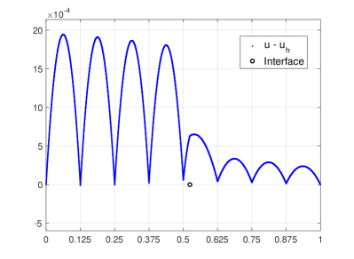
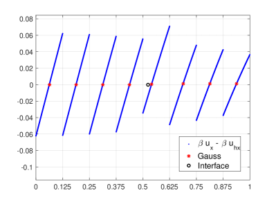
Figure 3: Error and flux error of $P_{1}$ IFE solution. $\beta=[1,5]$, $\alpha=\pi/6$, $\gamma=1$, $c=1$.

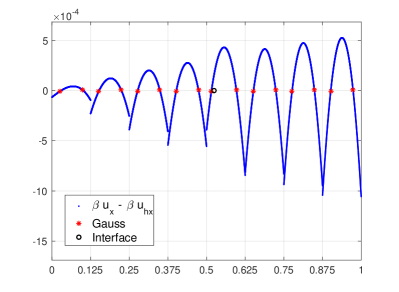
Figure 4: Error and flux error of $P_{2}$ IFE solution. $\beta=[1,5]$, $\alpha=\pi/6$, $\gamma=1$, $c=1$.

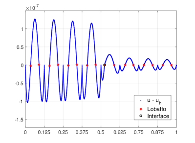
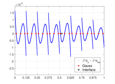
Figure 5: Error and flux error of $P_{3}$ IFE solution. $\beta^{-}=1$, $\beta^{+}=10$, $\alpha=\pi/6$, $\gamma=1$, $c=10$.

Example 5.2.

(Multiple interface points) In this example, we use IFE method to interface problems with multiple discontinuities. In particular, we consider the following function as the exact solution, where the coefficient function $\beta$ has two discontinuities at $\alpha_{1}$ and $\alpha_{2}$.

$$u(x)=\left\{\begin{array}[]{ll}\dfrac{1}{\beta_{1}}\cos(x),&\text{if}~{}~{}x\in[0,\alpha_{1}),\\ \dfrac{1}{\beta_{2}}\cos(x)+\left(\dfrac{1}{\beta_{1}}-\dfrac{1}{\beta_{2}}\right)\cos(\alpha_{1}),&\text{if}~{}~{}x\in(\alpha_{1},\alpha_{2}],\\ \dfrac{1}{\beta_{3}}\cos(x)+\left(\dfrac{1}{\beta_{1}}-\dfrac{1}{\beta_{2}}\right)\cos(\alpha_{1})+\left(\dfrac{1}{\beta_{2}}-\dfrac{1}{\beta_{3}}\right)\cos(\alpha_{2}),&\text{if}~{}~{}x\in(\alpha_{2},1].\\ \end{array}\right.$$ (5.2)

We set the interface points $\alpha_{1}=\frac{\pi}{6}$, and $\alpha_{2}=\frac{\pi}{6}+0.06$. They separate the domain into three subdomiains, on which the diffusion coefficients are chosen as $\beta_{1}=1$, $\beta_{2}=5$, $\beta_{3}=100$. It can be easy to verify that

$$\left[\!\left[u(\alpha_{i})\right]\!\right]=0,~{}~{}~{}\left[\!\!\left[\beta u^{(j)}(\alpha_{i})\right]\!\!\right]=0,~{}~{}\forall j\geq 1,~{}i=1,2.$$

$1/h$	$\|e_{h}\|_{node}$	$\|e_{h}\|_{L^{\infty}}$	$\|\beta e_{h}^{\prime}\|_{Gau}$	$\|e_{h}\|_{L^{2}}$	$\|e_{h}\|_{H^{1}}$
8	2.71e-05	1.92e-03	1.38e-03	9.67e-04	2.46e-02
16	5.26e-06	4.81e-04	3.48e-04	2.42e-04	1.24e-02
32	1.46e-06	1.20e-04	8.78e-05	6.06e-05	6.20e-03
64	3.86e-07	3.01e-05	2.20e-05	1.52e-05	3.11e-03
128	1.02e-07	7.53e-06	5.52e-06	3.82e-06	1.56e-03
256	2.56e-08	1.88e-06	1.38e-06	9.55e-07	7.81e-04
512	6.40e-09	4.71e-07	3.45e-07	2.39e-07	3.91e-04
rate	1.98	2.00	1.99	2.00	1.00

Table 4: Error of $P_{1}$ IFE Solution with $\beta=\{1,5,100\}$, $\alpha=\{\dfrac{\pi}{6},\dfrac{\pi}{6}+0.06\}$, $\gamma=1$, $c=1$.

$1/h$	$\|e_{h}\|_{node}$	$\|e_{h}\|_{L^{\infty}}$	$\|e_{h}\|_{Lob}$	$\|\beta e_{h}^{\prime}\|_{Gau}$	$\|e_{h}\|_{L^{2}}$	$\|e_{h}\|_{H^{1}}$
8	2.89e-08	6.70e-06	3.08e-07	9.77e-06	2.23e-06	1.17e-04
16	6.26e-09	8.84e-07	1.54e-08	1.45e-06	2.89e-07	3.05e-05
24	1.36e-09	2.67e-07	2.95e-09	3.67e-07	8.66e-08	1.35e-05
32	2.06e-10	1.14e-07	1.17e-09	1.55e-07	3.62e-08	7.53e-06
40	4.12e-11	5.87e-08	5.46e-10	9.17e-08	1.90e-08	4.93e-06
48	2.69e-11	3.54e-08	2.60e-10	4.67e-08	1.11e-08	3.46e-06
56	3.50e-11	2.22e-08	1.15e-10	2.93e-08	6.94e-09	2.53e-06
rate	3.95	2.93	3.95	2.97	3.00	1.97

Table 5: Error of $P_{2}$ IFE Solution with $\beta=\{1,5,100\}$, $\alpha=\{\dfrac{\pi}{6},\dfrac{\pi}{6}+0.06\}$, $\gamma=1$, $c=1$.

$1/h$	$\|e_{h}\|_{node}$	$\|e_{h}\|_{L^{\infty}}$	$\|e_{h}\|_{Lob}$	$\|\beta e_{h}^{\prime}\|_{Gau}$	$\|e_{h}\|_{L^{2}}$	$\|e_{h}\|_{H^{1}}$
8	2.01e-10	1.18e-07	1.66e-09	6.94e-08	5.51e-08	4.20e-06
10	9.06e-10	4.83e-08	5.41e-10	2.87e-08	2.26e-08	2.15e-06
12	7.44e-11	2.33e-08	2.16e-10	1.40e-08	1.10e-08	1.25e-06
14	2.94e-11	1.26e-08	9.99e-11	7.58e-09	5.92e-09	7.88e-07
16	1.00e-11	7.37e-09	5.13e-11	4.45e-09	3.47e-09	5.27e-07
18	1.70e-12	4.60e-09	2.85e-11	2.78e-09	2.16e-09	3.70e-07
20	1.27e-12	3.02e-09	1.69e-11	1.82e-09	1.42e-09	2.70e-07
rate	5.76	4.00	5.01	3.97	3.99	3.00

Table 6: Error of $P_{3}$ IFE Solution with $\beta=\{1,5,100\}$, $\alpha=\{\dfrac{\pi}{6},\dfrac{\pi}{6}+0.06\}$, $\gamma=1$, $c=1$.

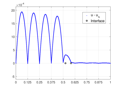
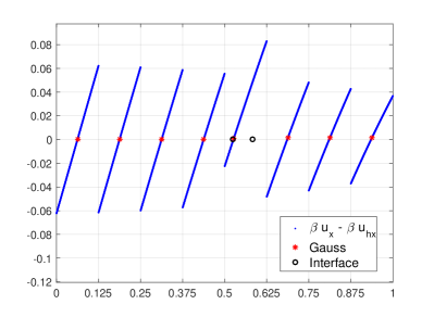
Figure 6: Error and flux error of $P_{1}$ IFE solution. $\beta=\{1,5,100\}$, $\alpha=\{\dfrac{\pi}{6},\dfrac{\pi}{6}+0.06\}$

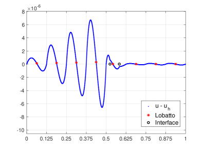
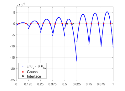
Figure 7: Error and flux error of $P_{2}$ IFE solution. $\beta=\{1,5,100\}$, $\alpha=\{\dfrac{\pi}{6},\dfrac{\pi}{6}+0.06\}$

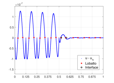
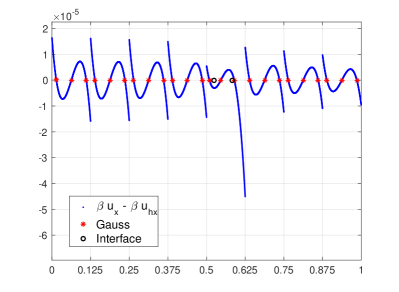
Figure 8: Error and flux error of $P_{3}$ IFE solution. $\beta=\{1,5,100\}$, $\alpha=\{\dfrac{\pi}{6},\dfrac{\pi}{6}+0.06\}$

Tables 4 - 6 report the numerical errors and convergence rates in different norms. Figures 6 - 8 demonstrate the superconvergence behavior on the roots of generalized Lobatto/Legendre polynomials. We note that, on the coarsest mesh which contains $8$ elements, the interface element contains two interface points. As the mesh size becomes smaller, the interface points are separated in different elements. This example shows the robustness of our scheme with respect to multiple coefficient discontinuities.

The numerical results for diffusion (only) interface problems are similar, except at mesh points there are only roundoff errors. We also conducted numerical experiments for different configuration of interface locations $\alpha$, and different sets of coefficients $\beta^{\pm}$, including large coefficient contrast. Similar superconvergence properties have been observed as the exemplified examples, hence we omit these data in the article.

6 Conclusion

In this article, we developed explicitly, the orthogonal IFE basis functions. First we constructed a set of bases for flux using (generalized) Legendre polynomials, then integrate to obtain basis functions for the primary unknown. The procedure is somewhat “reversed” from the classical approach in constructing IFE basis functions. The superconvergence behavior has been observed and proved for general elliptic interface problems in the one dimensional setting. At the roots of generalized Lobatto polynomial of degree $p+1$, the IFE solution is superconvergent to the exact solution with order $p+2$ (comparing with the optimal order $p+1$); at the roots of generalized Legendre polynomial of degree $p$, the derivative of the IFE solution is superconvergent to the derivative of the exact solution with order $p+1$ (comparing with the optimal order $p$). In addition, the convergent rate at all mesh points (including those of the interface element) is of order $p+2$ (comparing with the optimal order $p+1$). The idea presented in this article seems extendable to the two dimensional elliptic interface problems (at least for the tensor-product space case), which will be of interesting in future work.

Reference

References

- [1] S. Adjerid and T. Lin. Higher-order immersed discontinuous Galerkin methods. Int. J. Inf. Syst. Sci., 3(4): 555–568, 2007.
- [2] S. Adjerid and T. Lin. A -th degree immersed finite element for boundary value problems with discontinuous coefficients. Appl. Numer. Math., 59(6): 1303–1321, 2009.
- [3] S. Adjerid and T. C. Massey, Superconvergence of discontinuous Galerkin solutions for a nonlinear scalar hyperbolic problem, Comput. Methods Appl. Mech. Engrg., 195: 3331–3346, 2006.
- [4] I. Babuška and T. Strouboulis. The finite element method and its reliability. Numerical Mathematics and Scientific Computation. The Clarendon Press, Oxford University Press, New York, 2001.
- [5] I. Babuka, T. Strouboulis, C. S. Upadhyay, and S.K. Gangaraj, Computer-based proof of the existence of superconvergence points in the finite element method: superconvergence of the derivatives in finite element solutions of Laplace’s, Poisson’s, and the elasticity equations, Numer. Meth. PDEs., 12: 347–392, 1996.
- [6] J. Bramble and A. Schatz, High order local accuracy by averaging in the finite element method, Math. Comp., 31: 94–111, 1997.
- [7] S. C. Brenner and S. L. Ridgway, The mathematical theory of finite element methods, Texts in Applied Mathematics, 15 Springer-Verlag, New York, 1994.
- [8] Z. Cai, On the finite volume element method, Numer. Math., 58: 713–735, 1991.
- [9] B. Camp, T. Lin, Y. Lin, and W. Sun. Quadratic immersed finite element spaces and their approximation capabilities. Adv. Comput. Math., 24(1-4): 81–112, 2006.
- [10] W. Cao, C.-W. Shu, Y. Yang, and Z. Zhang, Superconvergence of discontinuous Galerkin methods for 2-D hyperbolic equations, SIAM. J. Numer. Anal., 53: 1651–1671, 2015.
- [11] W. Cao and Z. Zhang, Superconvergence of Local Discontinuous Galerkin method for one-dimensional linear parabolic equations, Math. Comp., 85: 63–84, 2016.
- [12] W. Cao, Z. Zhang, and Q. Zou, Superconvergence of any order finite volume schemes for 1D general elliptic equations, J. Sci. Comput., 56: 566–590, 2013.
- [13] W. Cao, Z. Zhang, and Q. Zou, Superconvergence of Discontinuous Galerkin method for linear hyperbolic equations, SIAM J. Numer. Anal., 52: 2555–2573, 2014.
- [14] W. Cao, Z. Zhang, and Q. Zou, Is -conjecture valid for finite volume methods?, SIAM J. Numer. Anal., 53(2): 942–962, 2015.
- [15] C. Chen and S. Hu, The highest order superconvergence for bi- degree rectangular elements at nodes- a proof of -conjecture, Math. Comp., 82: 1337–1355, 2013.
- [16] S. Chou and X. Ye, Superconvergence of finite volume methods for the second order elliptic problem, Comput. Methods Appl. Mech. Eng., 196: 3706-3712, 2007.
- [17] S.-H. Chou, D. Y. Kwak, and K. T. Wee. Optimal convergence analysis of an immersed interface finite element method. Adv. Comput. Math., 33(2):149–168, 2010.
- [18] J. Douglas, Jr. and T. Dupont. Galerkin approximations for the two point boundary problem using continuous, piecewise polynomial spaces. Numer. Math., 22: 99–109, 1974.
- [19] Y. Gong, B. Li, and Z. Li. Immersed-interface finite-element methods for elliptic interface problems with nonhomogeneous jump conditions. SIAM J. Numer. Anal., 46(1): 472–495, 2007/08.
- [20] W. Guo, X. Zhong and J. Qiu, Superconvergence of discontinuous Galerkin and local discontinuous Galerkin methods: eigen-structure analysis based on Fourier approach, J. Comput. Phys., 235: 458–485, 2013.
- [21] X. He, T. Lin, and Y. Lin. Approximation capability of a bilinear immersed finite element space. Numer. Methods Partial Differential Equations, 24(5): 1265–1300, 2008.
- [22] X. He, T. Lin, Y. Lin, and X. Zhang. Immersed finite element methods for parabolic equations with moving interface. Numer. Methods Partial Differential Equations, 29(2): 619–646, 2013.
- [23] R. Kafafy, T. Lin, Y. Lin, and J. Wang. Three-dimensional immersed finite element methods for electric field simulation in composite materials. Internat. J. Numer. Methods Engrg., 64(7): 940–972, 2005.
- [24] M. Kiek and P. Neittaanmki, On superconvergence techniques, Acta Appl. Math., 9: 175–198, 1987.
- [25] Z. Li. The immersed interface method using a finite element formulation. Appl. Numer. Math., 27(3): 253–267, 1998.
- [26] Z. Li, T. Lin, Y. Lin, and R. C. Rogers. An immersed finite element space and its approximation capability. Numer. Methods Partial Differential Equations, 20(3): 338–367, 2004.
- [27] Z. Li, T. Lin, and X. Wu. New Cartesian grid methods for interface problems using the finite element formulation. Numer. Math., 96(1): 61–98, 2003.
- [28] T. Lin, Y. Lin, and X. Zhang. Immersed finite element method of lines for moving interface problems with nonhomogeneous flux jump. In Recent advances in scientific computing and applications, volume 586 of Contemp. Math., pages 257–265. Amer. Math. Soc., Providence, RI, 2013.
- [29] T. Lin, Y. Lin, and X. Zhang. A method of lines based on immersed finite elements for parabolic moving interface problems. Adv. Appl. Math. Mech., 5(4): 548–568, 2013.
- [30] T. Lin, Y. Lin, and X. Zhang. Partially penalized immersed finite element methods for elliptic interface problems. SIAM J. Numer. Anal., 53(2): 1121–1144, 2015.
- [31] T. Lin, D. Sheen, and X. Zhang. A locking-free immersed finite element method for planar elasticity interface problems. J. Comput. Phys., 247: 228–247, 2013.
- [32] T. Lin, Q. Yang, and X. Zhang. A Priori error estimates for some discontinuous Galerkin immersed finite element methods. J. Sci. Comput., 65(3): 875–894, 2015.
- [33] T. Lin, Q. Yang, and X. Zhang. Partially penalized immersed finite element methods for parabolic interface problems. Numer. Methods Partial Differential Equations, 31(6):1925–1947, 2015.
- [34] A. H. Schatz, I. H. Sloan and L. B. Wahlbin, Superconvergence in finite element methods and meshes which are symmetric with respect to a point, SIAM J. Numer. Anal., 33: 505–521, 1996.
- [35] J. Shen, T. Tang, and L.-L. Wang. Spectral methods, volume 41 of Springer Series in Computational Mathematics. Springer, Heidelberg, 2011. Algorithms, analysis and applications.
- [36] V. Thomee, High order local approximation to derivatives in the finite element method, Math. Comp., 31: 652–660, 1997.
- [37] S. Vallaghé and T. Papadopoulo. A trilinear immersed finite element method for solving the electroencephalography forward problem. SIAM J. Sci. Comput., 32(4): 2379–2394, 2010.
- [38] L. B. Wahlbin. Superconvergence in Galerkin finite element methods, volume 1605 of Lecture Notes in Mathematics. Springer-Verlag, Berlin, 1995.
- [39] Z. Xie and Z. Zhang, Uniform superconvergence analysis of the discontinuous Galerkin method for a singularly perturbed problem in 1-D, Math. Comp., 79: 35–45, 2010.
- [40] J. Xu and Q. Zou, Analysis of linear and quadratic simplitical finite volume methods for elliptic equations, Numer. Math., 111: 469–492, 2009.
- [41] Y. Yang and C.-W. Shu, Analysis of optimal superconvergence of discontinuous Galerkin method for linear hyperbolic equations, SIAM J. Numer. Anal., 50: 3110–3133, 2012.
- [42] Z. Zhang, Superconvergence of Spectral collocation and p-version methods in one dimensional problems, Math. Comp., 74: 1621–1636, 2005.
- [43] Z. Zhang, Superconvergence of a Chebyshev spectral collocation method, Journal of Scientific Computing, 34: 237–246, 2008.
- [44] Z. Zhang, Superconvergence points of polynomial spectral interpolation, SIAM J. Numer. Anal., 50: 2966–2985, 2012.
- [45] O. C. Zienkiewicz and Y. K. Cheung, The Finite Element Method in Structural and Continuum Mechanics: Numerical Solution of Problems in Structural and Continuum Mechanics Vol. 1, European Civil Engineering Series, McGraw-Hill, 1967.