Real space renormalization of Majorana fermions in quantum nano-wire superconductors

Abstract

We develop the real space quantum renormalization group (QRG) approach for majorana fermions. As an example we focus on the Kitaev chain to investigate the topological quantum phase transition (TQPT) in the one-dimensional spinless p-wave superconductor. Studying the behaviour of local compressibility and ground-state fidelity, show that the TQPT is signalled by the maximum of local compressibility at the quantum critical point tuned by the chemical potential. Moreover, a sudden drop of the ground-state fidelity and the divergence of fidelity susceptibility at the topological quantum critical point are used as proper indicators for the TQPT, which signals the appearance of Majorana fermions. Finally, we present the scaling analysis of ground-state fidelity near the critical point that manifests the universal information about the TQPT, which reveals two different scaling behaviors as we approach the critical point and thermodynamic limit.

I Introduction

Majorana fermions (MFs) have attracted intense recent studies in condensed matter systemsNayak et al. (2008); Jason (2012). Based on exchange statistics, MFs are non-abelian anyons, in which particle exchanges in general do not commute, and they are nontrivial operationsAdy (2010); Chan et al. (2015). Furthermore, MFs can be used as qubits in topological quantum computation since they are intrinsically immune to decoherence Kitaev (2003); Bermudez et al. (2009). Since a MF is its own antiparticle, it must be an equal superposition of electron and hole states. Hence, superconducting systems are substantial candidates to search for such excitations. MFs can emerge in systems such as topological insulator-superconductor interfaces Fu and Kane (2008); Linder et al. (2010); Bermudez et al. (2010a); Pawlak et al. (2016), quantum Hall states with filling factor $5/2$ Gregory and Nicholas (1991), p-wave superconductors Read and Green (2000); Nozadze and Trivedi (2016), and half-metallic ferromagnets Duckheim and Brouwer (2011); Chung et al. (2011).

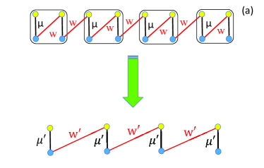
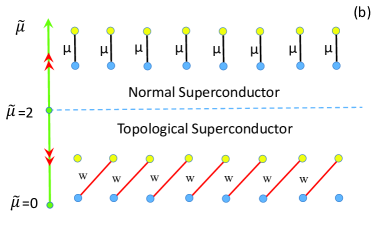
Figure 1: (Color online.) (a) Renormalization scheme of Majorana fermions in nanowire superconductor, (top) where a block of four MFs is mapped to (bottom) a renormalized pair of MFs. (b) Phase diagram of the one-dimensional Kitaev Model. In this diagram arrows show the flow of chemical potential under RG iteration. Each Majorana mode (yellow circle) for a given site is bound to its partner (blue circle) with strength $\mu$ for the normal phase, therefore there are no unbound modes. However for the topological phase there are leaving a free Majorana modes at the ends of a finite size system. In the topological superconductor phase the only existing bonds, with strength $w$, connect each Majorana mode (yellow circle) to its neighbour partner (blue circle).

There are various promising proposals for practical realisation of MFs in one or two dimensional systems. Among them, the one dimensional (1D) topological nano-wire superconductors (TSCs) Lutchyn et al. (2010); Oreg et al. (2010) provide experimental feasibility for the detection of MFs in hybrid superconductor-semiconductor wires Mourik et al. (2012); Deng et al. (2012). An egregious feature of a 1D TSC is the edge states (MFs), which appear at the ends of the superconducting wire. As shown by Kitaev Kitaev (2001), MFs can appear at the ends of 1D spinless p-wave superconducting chain when the chemical potential is less than a finite value, i.e. being in the topological regime. Recent progress in spin-orbit coupling research makes it possible to realize Kitaev chain in hybrid systems, such as superconductor-topological insulator interface Fu and Kane (2008), or semiconductor-superconductor heterostructure Sau et al. (2010); Jason (2012); Beenakker (2013). In such hybrids, the one dimensional spin-orbit coupling nanowire is proximity coupled to an ordinary s-wave superconductor Lutchyn et al. (2010); Oreg et al. (2010). It was predicted that there is a topological quantum phase transition (TQPT) in the system whenever a proper Zeeman field is applied, where the zero-energy modes and MFs appear in the topological non-trivial phase. All these experimental observations of the existence of Majorana fermions rely on the fact that the system is in a topological phase. Moreover, the observation of Majorana fermions has been reported using scanning tunneling microscopy Nadj-Perge et al. (2014).

In 1D, the MFs zero energy edge states, can be only found in the chain with open boundary condition, which due to the absence of the translational symmetry an analytical solution is not available. A conventional method to tackle this system is to solve the Bogoliubov-de Gennes equations, diagonalize the Hamiltonian in real space and obtain the energy spectrum as well as the quasi-particle wave functions. However, in the Bogoliubov-de Gennes formalism by increasing the lattice size, an analytical solution of the wave function and the fidelity are absent. Most importantly, since the topological phase can not be described within the Landau-Ginzburg symmetry breaking paradigm, investigation of such systems is very complicated. This fact has led to various types of approximations schemes, which can be roughly classified as variational, perturbative, numerical and renormalization group techniques. The difficulty of the task suggests that one should combine various techniques in order to come as close as possible to the exact solution.
In this paper, we show that how real space quantum renormalization group (QRG) approach is applicable to MFs in a wire with open ends to acquire the topological phase transition of the one dimensional p-wave superconductor. We emphasise that this is a technically simple method, which produces qualitative correct results when properly applied. Moreover, it is convenient to carry out analytical calculation in the lattice models and they are technically easy to extend to the higher dimensions. Furthermore, the advantage of the QRG formalism is its capability to evaluate the fidelity and fidelity susceptibility of a model without referring to the exact ground state of the model. Particularly, we calculate the local compressibility, ground-state fidelity, and fidelity susceptibility of the model as the robust geometric probes of quantum criticality. Ground-state fidelity is a measure, which shows the qualitative change of the ground state properties without the need to know a prior knowledge of the underlying phases. The universal scaling properties of fidelity and fidelity susceptibility have been investigated to extract the universal information of the topological phase transition.

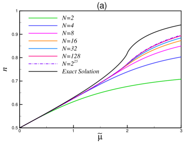
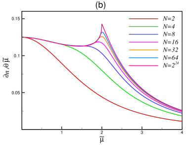
Figure 2: (Color online) (a) The particle density $n$ versus chemical potential $\mu$ for different system sizes (the exact solution data has been taken from Ref. Nozadze and Trivedi, 2016). (b) Derivative of particle density with respect to chemical potential (compressibility) versus $\mu$ for different lattice sizes.

The paper is organized as follows: In the next section, the model and majorana fermions are introduced. In Section III, the quantum renormalization approach is introduced to study the ground state phase diagram of the model. In section. IV, the density of particle and compressibility are investigated and section V is dedicated to analysis the ground state fidelity, fidelity susceptibility, and universal behaviour of the fidelity. Finally, we will discuss and summarize our results in Section VI.

II One Dimension Quantum Nano-Wire Superconductors

The Kitaev model, which was the first model realizing MFs in a one dimensional lattice Kitaev (2001); Bermudez et al. (2010b), is given by following Hamiltonian

$${\cal H}=\sum_{m=1}\Big{[} -\mu c^{\dagger}_{m}c_{m}-w(c^{\dagger}_{m}c_{m+1}+c^{\dagger}_{m+1}c_{m})$$ (1)

$$+\Delta(c_{m}c_{m+1}+c^{\dagger}_{m+1}c^{\dagger}_{m})\Big{]},$$

where $\mu$ is the chemical potential, $c^{\dagger}_{m}$ and $c_{m}$ are the electron creation and annihilation operators on site $m$. The superconducting gap, and hopping integral are defined by $\Delta$ and $w$ respectively. Since the time-reversal symmetry is broken in Eq. (1), we only consider a single value spin projection, i.e., effectively spinless electrons.
By introducing Majorana fermion operators as $a_{n}=c_{n}+c^{\dagger}_{n}$, and $b_{n}=i(c^{\dagger}_{n}-c_{n})$, which satisfy the communication relations: $\{a_{m},a_{n}\}=\{b_{m},b_{n}\}=2\delta_{m,n}$ and $\{a_{m},b_{n}\}=0$, the Hamiltonian, Eq. (1), takes the following form

$${\cal H}=\frac{-iw}{2}\sum_{n=1}\Big{[}\tilde{\mu}a_{n}b_{n}+(1-\tilde{\Delta})a_{n}b_{n+1}+(1+\tilde{\Delta})a_{n+1}b_{n}\Big{]},$$ (2)

where $\tilde{\Delta}=\Delta/w$, and $\tilde{\mu}=\mu/w$. It is well-known Kitaev (2001) that for the case $|\mu|<2w$, the ground state with MFs is fully realised and the system is called a topological superconductor, which shows qualitatively different behavior from the trivial phase, $|\mu|>2w$, without Majorana fermions.

III Quantum Renormalization Group

QRG is a method of studying systems with a large number of strongly correlated degrees of freedom. The main idea of this method is to decrease or thinning the number of degrees of freedom, so as to retain the information about essential physical properties of the system and eliminate those features which are not important for the considered phenomena. In the real space QRG, which is usually performed on lattice systems with discrete variables, one can divide the lattice into blocks which are treated as the sites of the new lattice. The Hamiltonian is divided into intra-block and inter-block parts, the former being exactly diagonalized, and a number of low lying energy eigenstates are kept to project the full Hamiltonian onto the new lattice Martín-Delgado and Sierra (1996); Langari (2004); Jafari and Langari (2006, 2007); Jafari et al. (2008); Jafari (2010, 2013); Langari and Karimipour (1997); Motrunich et al. (2001). In the new system there are less degrees of freedom, and the renormalized couplings are expressed as functions of the initial system’s couplings. Analysing the renormalized couplings (by tracing the flow of coupling constants), one can determine qualitatively the structure of the phase diagram of the underlying system, and approximately locate the critical points (unstable fixed points), and different phases (corresponding to stable fixed points). To implement the idea of QRG to Majorana fermions in quantum nano-wire superconductors, the Hamiltonian, Eq. (2), is divided into blocks of four MFs sites, as shown in Fig. 1(a). In this case, the total intra-blocks Hamiltonian is given by

$${\cal H_{B}} =\sum_{I=1}^{N/2}h^{B}_{I}$$ (3)

$$=\sum_{I=1}^{N/2}\frac{-iw}{2}\Big{[}\tilde{\mu}a_{1,I}b_{1,I}+\tilde{\gamma}a_{1,I}b_{2,I}+\tilde{\lambda}a_{2,I}b_{1,I}\Big{]},$$

where $h^{B}_{I}$ is the sub-Hamiltonian of individual block $I$, with $\tilde{\gamma}=1-\tilde{\Delta}$, and $\tilde{\lambda}=1+\tilde{\Delta}.$ The remaining part of the Hamiltonian is included in the inter-block part

$${\cal H_{BB}}=\frac{-iw}{2}\sum_{I=1}^{N/2}\Big{[}\tilde{\mu}a_{2,I}b_{2,I}+\tilde{\gamma}a_{2,I}b_{1,I+1}+\tilde{\lambda}a_{1,I+1}b_{2,I}\Big{]},$$ (4)

where we consider the open boundary chain.

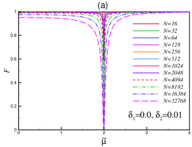
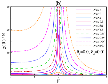
Figure 3: (Color online.) (a) Evaluation of the ground state fidelity of superconducting nanowire under quantum renormalization group for different chain sizes. (b) Fidelity of susceptibility per lattice size for different chain sizes.

The eigenstates and eigenvalues of the block Hamiltonian of four MFs are given by

$$|\psi_{0}\rangle=\frac{\alpha_{0}}{2}(a_{1}-ib_{1})|0^{a,b}_{1},0^{a,b}_{2}\rangle+\frac{\beta_{0}}{2}(a_{2}-ib_{2})|0^{a,b}_{1},0^{a,b}_{2}\rangle,~{}$$ (5)

$$|\psi_{1}\rangle=\beta_{1}|0_{1},0_{2}\rangle-\frac{\alpha_{1}}{4}(a_{1}-ib_{1})(a_{2}-ib_{2})|0^{a,b}_{1},0^{a,b}_{2}\rangle,$$

$$|\psi_{2}\rangle=\alpha_{1}|0_{1},0_{2}\rangle+\frac{\beta_{1}}{4}(a_{1}-ib_{1})(a_{2}-ib_{2})|0^{a,b}_{1},0^{a,b}_{2}\rangle,~{}$$

$$|\psi_{3}\rangle=\frac{\beta_{0}}{2}(a_{1}-ib_{1})|0^{a,b}_{1},0^{a,b}_{2}\rangle-\frac{\alpha_{0}}{2}(a_{2}-ib_{2})|0^{a,b}_{1},0^{a,b}_{2}\rangle,$$

and

$$E_{0}=-\frac{w}{2}(\tilde{\mu}+\sqrt{\tilde{\mu}^{2}+4});\;\;E_{1}=-\frac{w}{2}(\tilde{\mu}+\sqrt{\tilde{\mu}^{2}+4\tilde{\Delta}});\;\;$$ (6)

$$E_{2}=-\frac{w}{2}(\tilde{\mu}+\sqrt{\tilde{\mu}^{2}-4\tilde{\Delta}^{2}});\;\;E_{3}=-\frac{w}{2}(\tilde{\mu}-\sqrt{\tilde{\mu}^{2}+4}),$$

respectively. Here $|0^{a,b}_{1},0^{a,b}_{2}\rangle$ is the vacuum state of MFs in real space and

$$\alpha_{0}=-\frac{E_{0}/w}{\sqrt{(E_{0}/w)^{2}+1}},~{}~{}\beta_{0}=\frac{1}{\sqrt{(E_{0}/w)^{2}+1}},~{}~{}$$

$$\alpha_{1}=-\frac{E_{1}/w}{\sqrt{(E_{1}/w)^{2}+\tilde{\Delta}^{2}}},~{}~{}\beta_{1}=\frac{\tilde{\Delta}}{\sqrt{(E_{1}/w)^{2}+\tilde{\Delta}^{2}}}.$$

The projection operator $P^{I}_{0}$ for the $I$-th block is defined by

$$P_{0}^{I}=|\psi_{0}\rangle_{II}\langle\psi_{0}|+|\psi_{1}\rangle_{II}\langle\psi_{1}|,$$

and the renormalization of MFs operators are given by

$$P_{0}^{I}a_{1,I}P_{0}^{I}=(\alpha_{1}\beta_{0}+\alpha_{0}\beta_{1})a_{I},$$ (7)

$$P_{0}^{I}a_{2,I}P_{0}^{I}=(\beta_{0}\beta_{1}-\alpha_{1}\alpha_{0})a_{I},$$

$$P_{0}^{I}b_{1,I}P_{0}^{I}=(\alpha_{1}\beta_{0}-\alpha_{0}\beta_{1})b_{I},$$

$$P_{0}^{I}b_{2,I}P_{0}^{I}=(-\alpha_{1}\alpha_{0}-\beta_{0}\beta_{1})b_{I}.$$

It is remarkable that, two different type of Majorana fermion operators in real space treat nonconformingly under RG transformation. In this respect the effective Hamiltonian is expressed by

$${\cal H}^{eff}=P_{o}({\cal H_{B}}+{\cal H_{BB}})P_{0},$$ (8)

with total projector $P_{0}=\bigotimes_{I=1}^{N}P_{0}^{I}$. Thus, the effective Hamiltonian is obtained

$${\cal H}^{eff}= -\frac{i}{2}\sum_{n=1}w^{{}^{\prime}}\Big{[}\tilde{\mu}^{{}^{\prime}}a_{n}b_{n}+(-1+\tilde{\Delta}^{{}^{\prime}})a_{n}b_{n+1}$$ (9)

$$\hskip 56.9055pt-(1+\tilde{\Delta}^{{}^{\prime}})a_{n+1}b_{n}\Big{]}+e_{0},$$

where $w^{{}^{\prime}},~{}\tilde{\mu}^{{}^{\prime}}$, and $\tilde{\Delta}^{{}^{\prime}}$ are the renormalized coupling constants defined by the following QRG equations

$$w^{{}^{\prime}}=w[\alpha_{0}\beta_{0}+\tilde{\Delta}\alpha_{1}\beta_{1}],$$ (10)

$$\tilde{\Delta}^{{}^{\prime}}=-\frac{w}{w^{{}^{\prime}}}[\alpha_{1}\beta_{1}+\tilde{\Delta}\alpha_{0}\beta_{0}],$$

$$\tilde{\mu}^{{}^{\prime}}=\frac{(E_{1}-E_{0})-\mu(\alpha^{2}_{1}-\beta^{2}_{0})}{w^{{}^{\prime}}},$$

and $e_{0}=E_{0}-\mu\beta_{0}^{2}$ is a constant term as a function of coupling constants. Since the sign of hopping term and superconducting gap are changed, the effective Hamiltonian of the renormalized chain is not exactly similar to the original one. Therefore to get a self-similar Hamiltonian, we implement the unitary transformation $a_{n}\longrightarrow(-1)^{n}a_{n}$, and $b_{n}\longrightarrow(-1)^{n}b_{n}$, which is equivalent to $\pi$ rotation of even (or odd) sites around $z$-axis. We should emphasise that the commutation relations of MFs operators do not change under these transformation.

The stable and unstable fixed points of the QRG equations are obtained by solving the following equations $\tilde{\mu}^{{}^{\prime}}=\tilde{\mu}$, and $\tilde{\Delta}^{{}^{\prime}}=\tilde{\Delta}$. For simplicity we take $\Delta=w$, for which the Jordan Wigner transformation reconstructs the model to the Ising model in a transverse field (ITF). For $\tilde{\Delta}=1$ the renormalized couplings reduce to $w^{{}^{\prime}}=2w/\sqrt{4+\tilde{\mu}^{2}}$, and $\tilde{\mu}^{{}^{\prime}}=\tilde{\mu}^{2}/2$. It is remarkable to mention, although to compare with available exact results Rams and Damski (2011); GU (2010); Yu et al. (2009) we look at the QRG for the particular case of $w=\Delta$, our QRG equations can be considered for more general cases with different values of $w$ and $\Delta$ ($w\neq\Delta$). The QRG equations show that the stable fixed points are located at $\tilde{\mu}=0$ and $\tilde{\mu}\rightarrow\infty$ while $\tilde{\mu}_{c}=2$ stands for the unstable fixed point, which specifies the quantum critical point of the model. The phase diagram of the model has been shown in Fig. 1(b). As depicted, the chemical potential goes to zero for $\tilde{\mu}<\tilde{\mu}_{c}$ under QRG transformation, while it scales to infinity in the normal superconductor phase. The QRG equations, Eq. (LABEL:eq6), show the flow of $w$ to zero in a normal superconductor, which represents the renormalization of the energy scale while it goes to $1$ for the topological superconductor.

Fig. 1(b) shows that in the topological superconductor phase the only existing bonds connect $a_{n}$ to its neighbor $b_{n+1}$, and the Majorana modes at the ends of the chain are not coupled to anything. It manifests the presence of edge modes of a topological phase, which is the reason for the ground-state degeneracy that is not due to a symmetry. Furthermore, in the normal superconductor phase, each Majorana mode $a_{n}$ on a given site is bound to its partner $b_{n}$ with strength $\mu$, leaving no unbound modes, i.e. no edge state.

The quantum critical exponents associated with this quantum critical point can be obtained from the Jacobian of the QRG transformations by linearizing the QRG flow at the critical point ($\tilde{\Delta}=1$, and $\tilde{\mu}=2$),

$$J=\left(\begin{array}[]{cc}\frac{\partial\tilde{\mu}^{{}^{\prime}}}{\partial\mu}&\frac{\partial\tilde{\mu}^{{}^{\prime}}}{\partial\Delta}\\ \frac{\partial\tilde{\Delta}^{{}^{\prime}}}{\partial\mu}&\frac{\partial\tilde{\Delta}^{{}^{\prime}}}{\partial\Delta}\\ \end{array}\right),$$ (11)

which yields

$$J=\left(\begin{array}[]{cc}2&-1\\ 0&0\\ \end{array}\right).$$ (12)

The eigenvalues of the matrix of linearized flow are $\eta_{1}=2$ and $\eta_{2}=0$. The corresponding eigenvectors in the $|\tilde{\mu},\tilde{\Delta}\rangle$ coordinates are $|\eta_{1}\rangle=|1,0\rangle$, $|\eta_{2}\rangle=|1,2\rangle$. $|\eta_{1}\rangle$ shows the relevant direction which represents the direction of flow of chemical potential (see Fig. 1(b)). We have also calculated the correlation length exponents at the critical point ${\tilde{\mu}}_{c}=2$. In this respect, the correlation length diverges as $\xi\sim|\tilde{\mu}-2|^{-\nu}$ with the exponent $\nu=1$, which is expressed by $\nu=\ln[n_{B}]/\ln[{\rm d}\tilde{\mu}^{{}^{\prime}}/{\rm d}\tilde{\mu}]|_{\tilde{\mu}_{c}}$, and $n_{B}=2$ is the number of sites in each block.

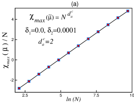
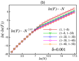
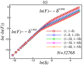
Figure 4: (Color online.) (a) The scaling behavior of the maximum of fidelity susceptibility in terms of system size. (b) Scaling behavior of the ground state fidelity, $\ln(-\ln(F))$, versus $\ln(N)$ close to the critical point $\tilde{\mu}_{c}=2$, for the Kitaev model with fixed $\delta=0.001$. (c) Scaling behavior of $\ln(-\ln(F))$ versus $\ln(\delta)$ for fixed size $N=2^{15}$ close to $\tilde{\mu_{c}}=2$.

IV particle density

The average local density of particles on site $n$ is

$$n(\tilde{\mu})=\frac{1}{N}\sum_{n=1}\langle\Psi_{0}|\frac{(a_{n}-ib_{n})(a_{n}+ib_{n})}{4}|\Psi_{0}\rangle,$$

and the ground state of the renormalized chain is related to the ground state of the original one by the transformation $P_{0}|\Psi_{0}^{{}^{\prime}}\rangle=|\Psi_{0}\rangle$. This leads to the particle density in the renormalized chain

$$n(\tilde{\mu},N) =\frac{1}{N}\sum_{n=1}\langle O^{{}^{\prime}}|P_{0}\Big{[}\frac{(a_{n}-ib_{n})(a_{n}+ib_{n})}{4}\Big{]}P_{0}|O^{{}^{\prime}}\rangle$$ (13)

$$=\frac{1}{2}+\gamma(0)n(\tilde{\mu}^{{}^{\prime}},\frac{N}{2}),$$

where $n(\tilde{\mu}^{{}^{\prime}},N/2)$ is the particle density in the renormalizd chain and $\gamma(0)$ is defined by $(2\alpha^{2}_{1}-1)/2$.

The average of the local density of particles has been ploted in Fig. 2(a) for different system sizes. It has been compared with the known exact result Nozadze and Trivedi (2016), which shows good agreement qualitatively. The compressibility, derivative of the local density of particles with respect to chemical potential, has been depicted in Fig. 2(b). The non-analytic behavior of the particle density at $\tilde{\mu_{c}}=2$ is high-lighted in the divergent behavior of the corresponding compressibility. It is to be noted that, although the compressibility has a singularity at the topological critical point in the thermodynamic limit ($N\rightarrow\infty$) this singularity can result from the singularity of density of states Thouless (1972). Therefore, to better understand the nature of topological phase transition in the model, the ground state fidelity of the model has been investigated in the next section.

V Ground State Fidelity

In the last few years, fidelity, which is a measure of the distance between quantum states, has been accepted as a new notion to characterize the drastic change of the ground states in quantum phase transition (QPT) point. Unlike traditional approaches, prior knowledge about the symmetries and order parameters of the model are not required in the fidelity notion to find out a QPT. In addition, fidelity has an interdisciplinary role, for example, it is related to the density of topological defects after a quench Damski (2005); Jafari (2016), decoherence rate of a test qubit interacting with a non-equilibrium environment Damski et al. (2011); Jafari and Akbari (2015), and orthogonality catastrophe of condensed matter systems Anderson (1967). In this section, we implement the formalism introduced in Refs. [Langari and Rezakhani, 2012] and [Amiri and Langari, 2013] to calculate the ground state fidelity of the nano-wire superconductor in terms of QRG. The advantage of the formalism is its adroitness to calculate the ground state fidelity of a model without referring to the exact ground state of the model.

The fidelity of ground state is defined by the overlap between the two ground state wave functions at different parameter values as follows

$$F=\langle\Psi_{0}(\tilde{\mu}-\delta_{1})|\Psi_{0}(\tilde{\mu}+\delta_{2})\rangle=\langle\Psi_{0}(\tilde{\mu}_{-})|\Psi_{0}(\tilde{\mu}_{+})\rangle,$$ (14)

where $\delta_{j}$ $(j=1,2)$ is a small deviation in the chemical potential. According to the renormalization transformation $P_{0}|\Psi_{0}^{{}^{\prime}}\rangle=|\Psi_{0}\rangle$, the fidelity of renormalized chain are related to the fidelity of original Hamiltonian by $F(\tilde{\mu},N)=\gamma_{1}F(\tilde{\mu}^{{}^{\prime}},N/2)$, where

$$\gamma_{1}=\Big{(}\alpha_{0}(\tilde{\mu}_{-})\alpha_{0}(\tilde{\mu}_{+})+\beta_{0}(\tilde{\mu}_{-})\beta_{0}(\tilde{\mu}_{+})\Big{)}^{\frac{N}{2}}.$$

The ground state fidelity of the model has been plotted versus chemical potential in Fig. 3(a) for different system sizes. Obviously, the ground state fidelity shows a sudden drop at the topological quantum critical point. Increasing the system size increases the depth of drop, which manifests unfailing drop in the thermodynamic limit. To determine more precisely the effect of quantum criticality on fidelity, we should extract universal information about the transition in addition to providing the location of the critical point. The universal information is defined by the critical exponents and reflects symmetries of the model rather than its microscopic details. For small system size, the universal information is explored in the fidelity susceptibility ($\chi$) approach,Zanardi and Paunković (2006); Rams and Damski (2011); Jafari (2016) which is defined by

$$\chi=2\lim_{\delta\rightarrow 0}\frac{1-F}{\delta^{2}},$$ (15)

in which $\delta_{1}=\delta_{2}=\delta/2$ is supposed. Fig. 3(a) represents fidelity susceptibility (FS) per lattice size ($\chi/N$) versus chemical potential, for various system sizes. Although $\chi/N$ does not show divergence for finite lattice sizes, the curves display marked anomalies with the height of peaks increasing with system size and diverges in the thermodynamics limit as the critical point is touched. The maximum of FS at finite size lattice $N$ obeys the scaling $\chi_{max}=N^{d_{a}^{c}}$ where $d_{a}^{c}$ denotes the critical adiabatic dimensionGU (2010); Yu et al. (2009). The scaling analysis of FS is figured out in Fig. 4(a). It is clearly verified that the scaling relation $\chi_{max}=N^{d_{a}^{c}}$ is satisfied with $d_{a}^{c}=2$. It is worth to mention that, the critical adiabatic dimension for the ITF is $d_{a}^{c}=2$ GU (2010); Yu et al. (2009). Furthermore, it has been shown that in the thermodynamic limit at fixed $\delta$, the fidelity scaling is given byRams and Damski (2011)

$$\ln F(\tilde{\mu},\delta)\sim-N|\delta|^{d\nu}g(\frac{\tilde{\mu}-\tilde{\mu_{c}}}{\delta}),$$ (16)

where $g$ is a scaling function. It has been shown thatRams and Damski (2011) at the critical point, fidelity is non-analytic in $\delta$ as $\ln F(\tilde{\mu_{c}},\delta)\sim-N|\delta|^{d\nu}$, while away from critical point for $|\delta|\ll|\tilde{\mu}-\tilde{\mu_{c}}|\ll 1$, it behaves as

$$\ln F(\tilde{\mu}_{c},\delta)\sim-N\delta^{2}|\tilde{\mu}-\tilde{\mu}_{c}|^{d\nu-2}.$$ (17)

The scaling behavior of fidelity around the critical point, $\tilde{\mu}\approx\tilde{\mu_{c}}$, is depicted in Fig. 4 (b). As seen, for small system sizes we cover the well known result Rams and Damski (2011) $\ln F\sim-N^{2}$, reported for ITF model in the finite size scaling case Zanardi and Paunković (2006). However for larger system sizes, we obtain $\ln F\sim-N$ conforming to Eq. (16). A more detailed analysis shows that the transition between the two regimes takes place when $N|\delta|\sim 1$. For this purpose in the Fig. 4(c), we plot the scaling behavior of $\ln(-\ln F)$ versus $\ln(\delta)$ for the fixed system size. We observe two distinct regimes, namely for $N|\delta|\ll 1$ that we have $\ln F\sim-\delta^{2}$, and for $N|\delta|\gg 1$ that we find $\ln F\sim-|\delta|$ in agreement with Eqs. (16) and (17). It should be mentioned that in our model $d=1$ and scaling verifies the correlation length exponent of $\nu=1$, which exactly corresponds to the correlation length exponent of ITF model.

VI Summary and conclusions

It is well-known that the real space quantum renormalization is applicable to non-exactly solvable systems such as XXZ model Martín-Delgado and Sierra (1996); Jafari and Langari (2006, 2007); Hubbard model Bhattacharyya and Sil (1995, 1998); Wang et al. (2002), as well as, XY model in a transverse field Langari (2004). In this work, we fully formulate quantum renormalization group for a system of Majorana fermions in the open boundary quantum nano-wire superconductors to obtain its universal behaviors, such as phase diagram, compressibility, ground state fidelity and scaling behavior of fidelity susceptibility. To compare our analytical approach to exact results, we concentrate on the special case with equal hopping and pairing terms, where the Kitaev model is mapped to the ITF. We conclude that real space quantum renormalization group procedure could reproduce exactly the location of the critical point and the critical exponents. The quantum renormalization group shows that in the topological phase ($\tilde{\mu}<\tilde{\mu}_{c}=2$), the chemical potential goes to zero by renormalization iteration while in the normal superconductor phase it flows to infinity. Furthermore, the results layout that the correlation length exponent and the critical adiabatic dimension are $\nu=1$ and $d^{c}_{a}=2$, respectively. Which corresponds to their counterpart in the Ising model in transverse field Rams and Damski (2011). Finally, we should emphasize that, the quantum renormalization method could be more expedient and more advantageous than the Bogoliubov-de Gennes formalism to carry out an analytical calculation in the lattice models, specifically in the disorder case and higher dimensions.

References

- Nayak et al. (2008) C. Nayak, S. H. Simon, A. Stern, M. Freedman, and S. Das Sarma, Rev. Mod. Phys. 80, 1083 (2008).
- Jason (2012) A. Jason, Reports on Progress in Physics 75, 076501 (2012).
- Ady (2010) S. Ady, Nature 464, 187 (2010).
- Chan et al. (2015) Y.-H. Chan, C.-K. Chiu, and K. Sun, Phys. Rev. B 92, 104514 (2015).
- Kitaev (2003) A. Y. Kitaev, Annals of Physics 303, 2 (2003).
- Bermudez et al. (2009) A. Bermudez, D. Patanè, L. Amico, and M. A. Martin-Delgado, Phys. Rev. Lett. 102, 135702 (2009).
- Fu and Kane (2008) L. Fu and C. L. Kane, Phys. Rev. Lett. 100, 096407 (2008).
- Linder et al. (2010) J. Linder, Y. Tanaka, T. Yokoyama, A. Sudbø, and N. Nagaosa, Phys. Rev. Lett. 104, 067001 (2010).
- Bermudez et al. (2010a) A. Bermudez, L. Amico, and M. A. Martin-Delgado, New Journal of Physics 12, 055014 (2010a).
- Pawlak et al. (2016) R. Pawlak, M. Kisiel, J. Klinovaja, T. Meier, S. Kawai, T. Glatzel, D. Loss, and E. Meyer, Npj Quantum Information 2, 16035 (2016).
- Gregory and Nicholas (1991) M. Gregory and R. Nicholas, Nuclear Physics B 360, 362 (1991).
- Read and Green (2000) N. Read and D. Green, Phys. Rev. B 61, 10267 (2000).
- Nozadze and Trivedi (2016) D. Nozadze and N. Trivedi, Phys. Rev. B 93, 064512 (2016).
- Duckheim and Brouwer (2011) M. Duckheim and P. W. Brouwer, Phys. Rev. B 83, 054513 (2011).
- Chung et al. (2011) S. B. Chung, H.-J. Zhang, X.-L. Qi, and S.-C. Zhang, Phys. Rev. B 84, 060510 (2011).
- Lutchyn et al. (2010) R. M. Lutchyn, J. D. Sau, and S. Das Sarma, Phys. Rev. Lett. 105, 077001 (2010).
- Oreg et al. (2010) Y. Oreg, G. Refael, and F. von Oppen, Phys. Rev. Lett. 105, 177002 (2010).
- Mourik et al. (2012) V. Mourik, K. Zuo, S. M. Frolov, S. R. Plissard, E. P. A. M. Bakkers, and L. P. Kouwenhoven, Science 336, 1003 (2012).
- Deng et al. (2012) M. T. Deng, C. L. Yu, G. Y. Huang, M. Larsson, P. Caroff, and H. Q. Xu, Nano Letters 12, 6414 (2012), pMID: 23181691.
- Kitaev (2001) A. Kitaev, Physics-Uspekhi 44, 131 (2001).
- Sau et al. (2010) J. D. Sau, R. M. Lutchyn, S. Tewari, and S. Das Sarma, Phys. Rev. Lett. 104, 040502 (2010).
- Beenakker (2013) C. W. J. Beenakker, Annu Rev Cond Phys 4, 113 (2013).
- Nadj-Perge et al. (2014) S. Nadj-Perge, I. K. Drozdov, J. Li, H. Chen, S. Jeon, J. Seo, A. H. MacDonald, B. A. Bernevig, and A. Yazdani, Science 346, 602 (2014).
- Bermudez et al. (2010b) A. Bermudez, L. Amico, and M. A. Martin-Delgado, New Journal of Physics 12, 055014 (2010b).
- Martín-Delgado and Sierra (1996) M. A. Martín-Delgado and G. Sierra, Phys. Rev. Lett. 76, 1146 (1996).
- Langari (2004) A. Langari, Phys. Rev. B 69, 100402 (2004).
- Jafari and Langari (2006) R. Jafari and A. Langari, Physica A 364, 213 (2006).
- Jafari and Langari (2007) R. Jafari and A. Langari, Phys. Rev. B 76, 014412 (2007).
- Jafari et al. (2008) R. Jafari, M. Kargarian, A. Langari, and M. Siahatgar, Phys. Rev. B 78, 214414 (2008).
- Jafari (2010) R. Jafari, Phys. Rev. A 82, 052317 (2010).
- Jafari (2013) R. Jafari, Physics Letters A 377, 3279 (2013).
- Langari and Karimipour (1997) A. Langari and V. Karimipour, Physics Letters A 236, 106 (1997).
- Motrunich et al. (2001) O. Motrunich, K. Damle, and D. A. Huse, Phys. Rev. B 63, 224204 (2001).
- Rams and Damski (2011) M. M. Rams and B. Damski, Phys. Rev. Lett. 106, 055701 (2011).
- GU (2010) S.-J. GU, Int. J. Mod. Phys. B 24, 4371 (2010).
- Yu et al. (2009) W.-C. Yu, H.-M. Kwok, J. Cao, and S.-J. Gu, Phys. Rev. E 80, 021108 (2009).
- Thouless (1972) D. J. Thouless, Journal of Physics C: Solid State Physics 5, 77 (1972).
- Damski (2005) B. Damski, Phys. Rev. Lett. 95, 035701 (2005).
- Jafari (2016) R. Jafari, J. Phys. A: Math. Theor. 49, 185004 (2016).
- Damski et al. (2011) B. Damski, H. T. Quan, and W. H. Zurek, Phys. Rev. A 83, 062104 (2011).
- Jafari and Akbari (2015) R. Jafari and A. Akbari, EPL (Europhysics Letters) 111, 10007 (2015).
- Anderson (1967) P. W. Anderson, Phys. Rev. Lett. 18, 1049 (1967).
- Langari and Rezakhani (2012) A. Langari and A. T. Rezakhani, New Journal of Physics 14, 053014 (2012).
- Amiri and Langari (2013) N. Amiri and A. Langari, physica status solidi (b) 250, 537 (2013).
- Zanardi and Paunković (2006) P. Zanardi and N. Paunković, Phys. Rev. E 74, 031123 (2006).
- Bhattacharyya and Sil (1995) B. Bhattacharyya and S. Sil, Journal of Physics: Condensed Matter 7, 6663 (1995).
- Bhattacharyya and Sil (1998) B. Bhattacharyya and S. Sil, Phys. Rev. B 57, 11831 (1998).
- Wang et al. (2002) J. X. Wang, S. Kais, and R. D. Levine, International Journal of Molecular Sciences 3, 4 (2002).