Parametric resonance induced chaos in magnetic damped driven pendulum

Abstract

A damped driven pendulum with a magnetic driving force, appearing from a solenoid, where ac current flows is considered. The solenoid acts on the magnet, which is located at a free end of the pendulum. In this system the existence and interrelation of chaos and parametric resonance is theoretically examined. Derived analytical results are supported by numerical simulations and conducted experiments.

Introduction: Chaos in damped driven pendulum system has a long standing history (see e.g. Refs. Gregory1 ; Gregory2 and references therein) and is applicable in vast variety of condensed matter problems Malomed ; Ruffo ; Alekseev1 ranging from Josephson junctions to easy-plane ferromagnets. Governing equation is written in the standard form:

$$\ddot{\alpha}=-{\Omega^{2}}\sin\alpha-q\dot{\alpha}+{f_{D}}\sin{\omega t}$$ (1)

where $\Omega$ and $q$ coefficients are usually fixed and $f_{D}$ is a one we control. Increasing control parameter $f_{D}$ period doubling Yorke ; Bevivino bifurcation scenario and transition to chaos takes place Hubbard ; Alekseev2 ; Harish . In all the mentioned papers control parameter is constant Hauptfleisch or a driving force has a time periodic singular character (kicked excited systems Popov ). In the present paper driving force is position angle $\alpha$ dependent, particularly, here, a realistic example of driven damped pendulum model is considered. In this context, driving force is of a magnetic origin, particularly a solenoid with ac current is acting on the magnet, which plays a role of a bob in a pendulum with a rigid rod (see Fig. 1). Therefore the amplitude of a harmonic force $f_{D}$ greatly depends on the distance between solenoid and the magnet, making it angle dependent in a non-trivial manner.

In the frames of the model (1) a possibility of onset of chaos has been examined analytically, numerically and experimentally. The similar model of magnetic pendulum has been studied long before doubochinski , particularly, different orientation of solenoid and magnet has been considered, where the orientation of the solenoid is perpendicular to the pendulum’s rod when the deviation angle is zero. In this case one gets quantization of amplitudes with no indication of onset of chaos, while in our case with parallel orientations of solenoid and pendulum in unperturbed position (see again Fig. 1) for some values of ac field and/or distance between solenoid and magnet chaos is observed due to the parametric resonance Belyakov . Thus the main peculiarity of our model is that the existence of parametric resonance is a necessary condition for the onset of chaos in the system.

Theoretical Model: In my experiments and numerical simulations the magnet is rigidly fixed in the place of a bob of the pendulum in such a way that the directions of its magnetic moment and the rod of pendulum coincides. Approximating solenoid and magnet as point-like magnetic moments ($\overrightarrow{L}_{1}$ and $\overrightarrow{L}_{2}$, respectively), one can readily write down their dipolar interaction energy as follows:

$$U=\frac{\mu_{0}}{4\pi}\left(\frac{3\cdot(\overrightarrow{L}_{1}\cdot\overrightarrow{r})(\overrightarrow{L}_{2}\cdot\overrightarrow{r})}{{r^{5}}}-\frac{\overrightarrow{L}_{1}\cdot\overrightarrow{L}_{2}}{r^{3}}\right)$$

where $\overrightarrow{r}\equiv(x,~{}y)$ is a radius vector of magnet with respect to the solenoid, $r=\sqrt{x^{2}+y^{2}}$. Taking into account now that ac current is flowing into the solenoid and the magnet is attached at the free end of the pendulum one can write for the components of magnetic moments following expressions (see also Fig. 1):

$${L_{1x}}=0,\quad{L_{2x}}=-{L_{2}}\frac{x}{\ell},$$

$${L_{1y}}={L_{1}(t)},\quad{L_{2y}}={L_{2}}\frac{{r_{0}}+\ell-y}{\ell}$$ (2)

where $\ell$ is the length of the pendulum and $r_{0}$ is distance between magnet and solenoid when the deviation angle from vertical direction is zero (that is a minimal distance position between solenoid and magnet).

Plugging (2) into (1) we find $F_{x}$ and $F_{y}$ components of the forces acting on the magnet:

$${F_{x}}=-\frac{\partial{U}}{\partial{x}}\qquad{F_{y}}=-\frac{\partial{U}}{\partial{y}}$$

we write Newton’s second law for tangential axis of the pendulum as follows:

$$m\ddot{\alpha}\ell={F_{x}}\cos{\alpha}+{F_{y}}\sin{\alpha}-mg\sin{\alpha}-q\dot{\alpha}$$ (3)

where a damping proportional to velocity has been included and $m$ is a mass of the magnet. We do not write here explicit expressions for components of the force because of their cumbersomeness, although their complete expressions will be used for numerical simulations, while for analytics we just linearize (3) for small deviation angles $\alpha$ and approximate $r\rightarrow r_{0}$:

$$\ddot{\alpha}=-{\alpha}\left(\frac{g}{\ell}+\frac{12{L_{1}}(t){L_{2}}}{mr_{0}^{5}}+\frac{2{L_{1}}(t){L_{2}}}{m{\ell^{2}}{r_{0}^{3}}}\right)-q\dot{\alpha}$$ (4)

where ${L_{1}}(t)\equiv{L^{0}_{1}}\cos{2\omega t}$ because of the ac current (with $2\omega$ frequency) flowing through the solenoid. Then let us denote

$$\omega_{0}=\sqrt{\frac{g}{\ell}},\qquad h={L^{0}_{1}}\left(\frac{12{L_{2}}}{mr_{0}^{5}}+\frac{2{L_{2}}}{m{\ell^{2}}{r_{0}^{3}}}\right)$$ (5)

and reduce (4) to the following equation:

$$\ddot{\alpha}=-{\alpha}({\omega_{0}^{2}}+h\cos{2\omega t})-q\dot{\alpha}$$ (6)

which is just a Mathieu equation if one sets damping to zero.

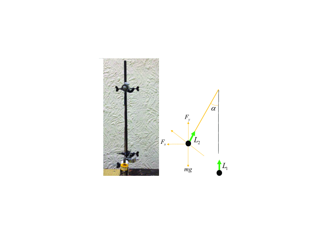
Figure 1: Experimental setup (left) and schematics (right) for driven damped magnetic pendulum. $L_{1}$ is a dipolar moment of solenoid, $L_{2}$ is a dipolar moment of the magnet. $\alpha$ is a deviation angle of the pendulum from vertical. $F_{x}$ and $F_{y}$ are $x$ and $y$ components of magnetic force acting on the magnet.

The presence of parametric resonance in (6) is examined in Ref. Landau for driving frequencies $\omega$ close to pendulum oscillation frequency $\omega_{0}$. Actually, similar analysis could be done for arbitrary $\omega$ and the existence of parametric resonance in the system will cause undamped oscillations, chaos and some more interesting phenomena. In order to find out what conditions should be fulfilled for this to occur, we should seek the solution of equation (6) in the following form:

$${\alpha}=a(t)\cos{\omega t}+b(t)\sin{\omega t}$$ (7)

considering $a(t)$ and $b(t)$ as slow functions of time and neglecting their second derivatives, (6) is simplified to the following form:

$$X\cos{\omega t}+Y\sin{\omega t}=0$$ (8)

Where coefficients $X$ and $Y$ both depend on $a(t)$ and $b(t)$. For the equation to be true, both coefficients should be equal to zero. Thus we get a set of two equations, where our goal is to find the regimes of parametric resonance. For this, we should seek for the solution in the exponential form $a(t)=Ae^{st}$ and $b(t)=Be^{st}$ and two equations are derived:

$$A\cdot(2s\omega+q\omega)-B\cdot({\omega_{0}}^{2}+\frac{h}{2}-{\omega}^{2})=0$$

$$A\cdot({\omega}^{2}-\frac{h}{2}-{\omega_{0}}^{2})-B\cdot(2s\omega+q\omega)=0.$$ (9)

Finally we get from the compatibility condition:

$$s=\frac{{\omega_{0}}^{2}+\frac{h}{2}-{\omega}^{2}-q\omega}{2\omega}$$ (10)

Considering parametric instability growth rate $s$ to be positive, the instability condition will be:

$$h\geq 2\mid w^{2}-{w_{0}}^{2}+2q\omega\mid.$$ (11)

This defines the limits of existence of parametric resonance and its dependence on various parameters, but all of these is valid for small angles. In order to get the full dynamics we should solve differential equation (3) in a full range of angles. $F_{x}$ and $F_{y}$ components of magnetic force are known from derivative of dipole-dipole energy. If we do not consider the angle as small, we will not be able to make the approximations that has been done before. In general, $F_{x}$ and $F_{y}$ components are very complicated expressions and it is impossible to solve the equation (3) analytically. Therefore I performed numerical simulations using Matlab.

Numerical simulations: Our next goal is to prove theoretically the existence of chaos in the system, considering deviation angles as arbitrary. The given equation of motion (3) has been solved using $ode45$ toolbox of Matlab program with an initial guess that chaos should occur when parametric resonance for small angles takes place. And this appears to be true, because as the numerical simulations show, when there is parametric instability in the system, it is always chaotic. To prove the existence of chaos, the common way is to check, whether changing any parameter insignificantly, the difference between the first and second measurement of some variable increases exponentially in time. In other words, Lyapunov exponent should be calculated in order to analyze the behavior of chaotic motion. To calculate the exponent, one has to deviate e.g. initial angle $\alpha(0)$ by small value making it $\alpha^{\prime}(0)$ and as time evolves, divide the resulting difference between angles $\alpha(t)$ and $\alpha^{\prime}(t)$ on initial deviation. Taking out logarithm from this, dividing on time and averaging the results upon the initial deviations Lyapunov exponent of the process could be defined. Positive exponent is an obvious indication of the presence of chaos and one should look at the simultaneous presence of parametric resonance condition in the system.

Another test to check the relation between parametric resonance and chaos in our case of magnetic pendulum is to look whether the system performs large angle oscillations starting from initial insignificant deviations. In other words, if we give the pendulum very small initial angle, for example 0.0001 rad, and after some time it starts to oscillate with normal angles, this means that there is parametric resonance and chaos in the system. The latter scenario is observed in experiments when the system is in parametrically unstable regime. In Fig. 2 solid blue line indicates theoretical boundary line of parametric resonance, so it is also boundary of chaos and stability. Red dots are boundaries of chaos from numerical simulations, so the discrepancy between theory and numerical calculations is really small. We also indicate by error bar experimental range where transition from stability to chaos occurs.

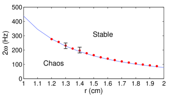
Figure 2: Comparison of theoretical and numerical results for finding the boundaries of parametric resonance and chaos. Solid line is theoretical curve according to (11) and red dots are plotted using numerical simulations. Error bars show the boundary area of chaos in experiments.

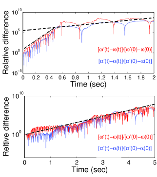
Figure 3: In both graphs blue and red solid lines show relative angle and angular velocity differences, respectively, versus time. Black dashed line follows from theoretical estimate of parametric resonance growth rate (10) equal to $s=3.63$. Driving frequency in both graphs is $29$ Hz and pendulum parameters are indicated in the text. Initial angle is very small $0.0001$ rad. In case of upper panel initial large growth rate with the exponent $\approx 23$ (dotted-dashed line) is caused by the fact that at $t=0$ current starts to flow in solenoid instantly. Bottom graph shows the same relative differences of angles and velocities, but when we multiply dipolar moment of solenoid on the factor $1-\exp(-t)$, it prevents current (and therefore force) to gain large values almost instantly.

In Figs. 3 and 4 the evolution of relative differences of the pendulum angle $\alpha$ and angular velocity $\dot{\alpha}$ ($\omega$) are presented. For instance, in case of relative angle difference we use for its calculation the formula $\left[\alpha^{\prime}(t)-\alpha(t)\right]/\left[\alpha^{\prime}(0)-\alpha(0)\right]$. We evaluate the dynamics from two small initial values, e.g. $\alpha(0)=0.0001$ and $\alpha^{\prime}(0)=0.0001001$ and average upon different initial deviations. Lyapunov exponent values are as follows: for angles we get the exponent value equal to $3.47$ and for angular velocities it is $3.56$ which in good approximation coincides with parametric instability growth rate $s=3.63$, calculated from formula (10). As seen from upper graph of Fig. 3, in the beginning we have rapid growth of relative angle and velocity differences, which is characterized by a value of Lyapunov exponent equal to $23$, and it is quite different than theoretical growth rate. This effect happens because in numerical experiments at $t=0$ current starts to flow in solenoid abruptly, therefore a force of finite value instantly appears on magnet, and this is the cause of strange behaviour of pendulum. In order to exclude such a scenario we multiply the dipolar moment of solenoid ${L_{1}}(t)\equiv{L^{0}_{1}}\cos{2\omega t}$ on the time dependent factor $1-\exp(-t)$, modelling smooth growth of the current in the solenoid. One can observe the result on the bottom panel of Fig. 3. As seen, no rapid growth takes place in the beginning of the time, because, the current (and therefore force) starts to increase slowly and the value of the Lyapunov exponent coincides with theoretical growth rate (black dashed line).

No calculations of Lyapunov exponent were made using scenario displayed on the bottom panel, it is only used to prove and explain the reason of rapid growth in the upper panel of Fig. 3. In calculations of Lyapunov exponent of angles and velocities the beginning of time where rapid growth takes place has not been considered, and calculated Lyapunov exponent coincides with theoretical growth rate $s=3.63$. Theoretical and numerical results are really close in Fig. 3, that is because of the fact that the initial deviation angle of the pendulum is small.

While in Fig. 4 the initial deviation angle is around $1$ rad and Lyapunov exponent is equal to $1.55$ and it does not coincide with theoretical growth rate $s=3.63$. This fact was predictable, because pendulum actually spends little time at small deviation angles where parametrical instability is in force. However, the range of stabilty-chaos diagram plotted in Fig. 2 is still valid for large initial deviation angles.

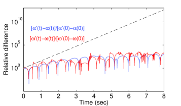
Figure 4: The same as in Fig. 3 except initial angle, which is 1 rad. This is not a small angle and that is why numerical results do not fit with theoretical growth rate indicated by dashed line. Lyapunov exponent in this case is $1.55$ and theoretical growth rate is $s=3.63$.

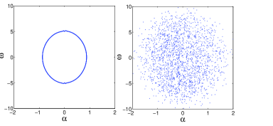
Figure 5: Left: Poincare graph when the system is not chaotic corresponding to the minimal distance between solenoid and magnet $r_{0}=22$ mm. Right: Poincare graph in case of chaos when $r_{0}=14$ mm. The initial angle in both cases is large ($\alpha(0)=1$ rad), and time step is the period of oscillations of free pendulum with an initial $1$ rad angle. Other parameters of the system are given in the text.

Here are the parameters for figures 3 and 4: minimal distance between magnet and solenoid is $r_{0}=14mm$, the length of the pendulum is taken as $\ell=28$ cm, dipolar moment amplitude of solenoid is $L_{1}^{0}=1.8$ $A\cdot{m^{2}}$, dipolar moment of the magnet is $L_{2}=0.2$ $A\cdot{m^{2}}$, mass of the magnet is $m=0.05$ kg, damping coefficient is taken as $q=0.01$ and ac current frequency is $2\omega=58\pi$.

In Fig. 5 two Poincare graphs are displayed, both of them express the system dynamics with the same initial parameters, except minimal distance from solenoid to the magnet: for left graph $r_{0}=22$ mm, which corresponds to the regular evolution, while at the right the chaotic behavior is observed for $r_{0}=14$ mm. In both cases the initial angle is large (1 rad) and the time period of plotting dots is the own oscillation period of the free pendulum with the same parameters. If the time period of plotting dots were the oscillation period in the presence of magnetic field and not the own oscillation period of the free pendulum, Poincare graph would be a point for the parameters of left graph of Fig 5 (non-chaotic regime). Poincare graphs are only displayed for the cases where the initial angle is large, because in case of small angles it is clear that when parametric resonance occurs, the system is unavoidably chaotic.

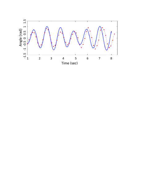
Figure 6: Comparison of theoretical model (blue solid line) and experimental one in case of regular dynamics. Red dots are experimental data and red dashed line is for guide of eyes.

Experiments: In Fig. 1 experimental magnetic pendulum is displayed. All parameters are easily measurable except dipolar moments of solenoid and magnet. For this purpose we have used magnetic field sensor and the measurements were made in different locations (more than $50$ locations). Applying then regression formula we have estimated values of dipolar moments. The experimental parameters which are used in numerical simulations are given in the previous section. While conducting experiments slow motion camera has been used in order to track pendulum motion. After the data has been processed on the computer and points have been plotted on theoretical graph (see Fig. 6). It has been taken into account that experimental pendulum is not a mathematical one, and thus (3) has been rewritten for the physical pendulum case. Besides that, experimentally, damping proportional to the velocity is to be taken into account. The damping coefficient $q$ was measured as follows: the time needed for damping from initial angle is recorded, and then it is compared to numerical calculations made in Matlab with different damping coefficients. For the coefficient $q=0.01$ the damping took the same time as in the experiment. In Fig. 6 a comparison of theoretical model and experiment has been made in case of nonchaotic regime and one can clearly see that theory and experiment is well-fitted. The difference between them of course grows with time, because there are some experimental errors, which constantly act on the motion characteristics. The main error is that dipoles in reality have size, especially solenoid while in theoretical model we have made an assumption that they are point-like.

The video in supplemental material is recorded for the case when the system is chaotic. We have zero initial deviation. When we let the current flow into the solenoid the pendulum start large amplitude oscillations. From a very small initial angle system stars large amplitude oscillations, so it proves the existence of parametric resonance and consequently the chaos in the system.

Conclusions: We have proved and examined the existence and interrelation of parametric resonance and chaos in the system of magnetic pendulum. Lyapunov exponents were calculated using numerical simulations and were compared with theoretical growth rate. Lyapunov exponent for small angles (angular velocities) matches with theoretical growth rate and for large angles it is different, as it was expected. The overall conclusion is that our magnetic pendulum system is chaotic only when the conditions for parametric resonance are fulfilled. Besides that, experiments have been carried out and give a very good agreement with theoretical model and numerical simulations.

I would like to give special thanks to T. Gachechiladze and G. Mikaberidze for very useful discussions.

References

- (1) G.L. Baker and J.P. Gollub, Chaotic Dynamics: An Introduction, Cambridge University Press, (1990).
- (2) G.L. Baker and J.A. Blackburn, The Pendulum: A Case Study in Physics, Oxford University Press (2005).
- (3) G. Filatrellaa, B.A. Malomed, and S. Pagano, Phys. Rev. E 65, 051116 (2002).
- (4) F. Cagnetta, G. Gonnella, A. Mossa, S. Ruffo, EPL (Europhysics Letters), 111, 10002, (2015).
- (5) K.N. Alekseev and F.V. Kusmartsev, Physics Letters A, 305, 211, (2002).
- (6) E. Sander and J.A. Yorke, Ergod. Th. Dynam. Sys, 31, 1249, (2011).
- (7) J. Bevivino, Dynamics at the Horsetooth, 1, (2009).
- (8) J.H. Hubbard, Amer. Math. Monthly, 106, 741, (1999).
- (9) J. Isohätälä, K.N. Alekseev, L.T. Kurki, and P. Pietilainen, Phys. Rev. E, 71, 066206, (2005).
- (10) R. Harish, S. Rajasekar, and K. P. N. Murthy, Phys. Rev. E 65, 046214, (2002).
- (11) H. Hauptfleisch, T. Gasenzer, K. Meier, O. Nachtmann, and J. Schemmel, American Journal of Physics, 78, 555 (2010).
- (12) V. Damgov and I. Popov, OPA (Overseas Publishers Association), 4, 99 (2000).
- (13) D.B. Doubochinski, Ya.B. Duboshinsky et al., Zh. Tech. Fiz. 49, 1160 (1979) [Sov. Phys. - Tech. Phys. 24, 642 (1979)]
- (14) A. Belyakov, A. Seyranian, A. Luongo, Physica D, 238, 1589, (2009).
- (15) L.D. Landau, E.M. Lifshitz, Mechanics. Pergamon Press, (1969).