Gravitational waves from cosmological first order phase transitions

Abstract:

First order phase transitions in the early Universe generate gravitational waves, which may be observable in future space-based gravitational wave observatiories, e.g. the European eLISA satellite constellation. The gravitational waves provide an unprecedented direct view of the Universe at the time of their creation. We study the generation of the gravitational waves during a first order phase transition using large-scale simulations of a model consisting of relativistic fluid and an order parameter field. We observe that the dominant source of gravitational waves is the sound generated by the transition, resulting in considerably stronger radiation than earlier calculations have indicated.

1 Introduction

The gravitational wave window to the Universe is about to open. The advanced LIGO gravitational wave laser interferometry detector [1] has just started collecting data, and will soon be joined by advanced VIRGO [2] and KAGRA [3] detectors. These are expected to detect gravitational wave signals from merging neutron star binaries and possibly from supernovae.

In the early Universe there are several processes which may generate observable gravitational radiation, such as inflation, cosmic strings or other topological defects and first order phase transitions. These may be observable in proposed future space-based detectors, in the first place the European eLISA satellite constellation [4], scheduled for launch in 2034. It consists of three satellites in a triangular formation, which forms a laser interferometer with arm length of order 1 million kilometers. Due to its large size, eLISA is sensitive to radiation at much lower frequencies than the Earth-based interferometers, in the range $10^{-4}$–1 Hz. eLISA technology demonstrator, LISA pathfinder, will be launched in December 2015.

eLISA and other proposed space-based interferometers have the right frequency response for the detection of radiation form first order phase transitions at the electroweak scale and above. In the Standard Model the electroweak transition is known to be a cross-over [5, 6, 7, 8], which does not lead to a gravitational wave signal. However, a strong first order phase transition is possible in various extensions of the Standard Model [9, 10, 11, 12, 13, 14, 15].

A first order phase transition proceeds as follows [16, 17, 18]: due to the metastability associated with the first order phase transitions, the high-temperature “symmetric” phase supercools until critical bubbles of the low-temperature “broken” phase are spontaneously nucleated. These bubbles grow until the bubble walls collide with other bubbles and the phase transition is completed. The growing bubble walls push the fluid along, causing hydrodynamical flows, which may persist long after the bubbles have vanished.

The generation of gravitational waves requires that the system has a non-vanishing quadrupole moment. Thus, a single spherical bubble does not generate radiation. However, when the bubbles collide the spherical symmetry is broken and gravitational radiation is possible. In the widely used semi-analytical envelope approximation [19, 20, 21, 22, 23] the fluid is modeled to behave like the order parameter field, and the gravitational waves are generated as the bubbles collide. Thus, the gravitational waves originating from fluid flows after the transition has completed are ignored.

In this work we describe the phase transition using an effective relativistic fluid + scalar order parameter model, where the model parameters can be fixed to thermodynamic quantities of the original theory. Using large-scale numerical simulations, we observe that the dominant source of the gravitational radiation are the acoustic waves generated by the bubbles: the sound of the transition. The role of the sound waves was originally suggested in ref. [24]. Acoustic waves remain active long after the transition itself has completed, for up to the Hubble time. The resulting gravitational radiation can be orders of magnitude stronger than indicated by earlier results. Our main results have been reported in [25, 26].

2 Effective theory

We describe the matter in the early universe with a relativistic fluid coupled with a scalar order parameter field $\phi$ which drives the transition. We note that $\phi$ needs not to correspond to any fundamental field of some underlying microscopic theory. We use a potential of the form

$$V(\phi,T)=\frac{1}{2}\gamma(T^{2}-T_{0}^{2})\phi^{2}-\frac{1}{3}\alpha T\phi^{3}+\frac{1}{4}\lambda\phi^{4},$$ (1)

where the parameters are adjusted to give the desired thermodynamic properties of the transition. The rest-frame pressure $p$ and energy density $\epsilon$ are

$$\epsilon=3aT^{4}+V(\phi,T)-T\frac{\partial V}{\partial T},~{}~{}~{}~{}p=aT^{4}-V(\phi,T)$$ (2)

with $a=(\pi^{2}/90)g$, where $g$ is the effective number of relativistic degrees of freedom. For details, we refer to [26].

The energy-momentum tensor of the field-fluid system is

$$T^{\mu\nu}=\partial^{\mu}\phi\partial^{\nu}\phi-{\textstyle\frac{1}{2}}g^{\mu\nu}(\partial\phi)^{2}+\left[\epsilon+p\right]U^{\mu}U^{\nu}+g^{\mu\nu}p\equiv T^{\mu\nu}_{\rm field}+T^{\mu\nu}_{\rm fluid}$$ (3)

where $U^{\mu}$ is the 4-velocity of the fluid. The equations of motion are now obtained from the energy-momentum conservation $\partial_{\mu}T^{\mu\nu}=0$, where we introduce a non-unique coupling term permitting the transfer of energy and momentum between the field and the fluid [27, 28, 26]:

$$\partial_{\mu}T^{\mu\nu}_{\rm field}=-\partial_{\mu}T^{\mu\nu}_{\rm fluid}=\eta U^{\mu}\partial_{\mu}\phi\partial^{\nu}\phi.$$ (4)

The final equations of motion can now be written as [25]

$$-\ddot{\phi}+\nabla^{2}\phi-\frac{\partial V}{\partial\phi} ={{\eta}}W(\dot{\phi}+v^{i}\partial_{i}\phi)$$ (5)

$$\dot{E}+\partial_{i}(Ev^{i})+p[\dot{W}+\partial_{i}(Wv^{i})]-\frac{\partial V}{\partial\phi}W(\dot{\phi}+v^{i}\partial_{i}\phi) ={\eta}W^{2}(\dot{\phi}+v^{i}\partial_{i}\phi)^{2}$$ (6)

$$\dot{Z}_{i}+\partial_{j}(Z_{i}v^{j})+\partial_{i}p+\frac{\partial V}{\partial\phi}\partial_{i}\phi =-{\eta}W(\dot{\phi}+v^{j}\partial_{j}\phi)\partial_{i}\phi.$$ (7)

Here $W$ is the relativistic $\gamma$-factor, $v^{i}=U^{i}/W$ the fluid 3-velocity, $E=W\epsilon$ is the fluid energy density, and $Z_{i}=W^{2}(\epsilon+p)v_{i}$ momentum density. The right-hand sides of the equations (5–7) describe the coupling of the field and the fluid, with the strength parametrized by $\eta$.

The traceless and transverse part of the energy-momentum tensor generates metric perturbations:

$$\ddot{h}_{ij}-\nabla^{2}h_{ij}=16GT_{ij}^{TT}$$ (8)

We use the procedure detailed in [29] to project the transverse part.

We refer to [25] for the details of the lattice implementation of the equations of motion. For the scalar field, we use the standard leapfrog update, and the the relativistic fluid is evolved using the donor cell advection method [30]. The lattice volumes vary up to $4200^{3}$, using up to 24 000 cores on a Cray XC-30. A somewhat different lattice implementation of the fluid+field system is presented in ref. [31].

3 Results

We show here results from simulations corresponding to relatively weak transition with latent heat ${\cal L}=(9/40)T_{c}^{4}$. The phenomenological field-fluid coupling parameter is set to $\eta/T_{c}=0.1$, $0.15$ and $0.2$. For the detailed simulation parameters we refer to [26].

When $\eta$ is small, the coupling between the field and the fluid is small, allowing the bubble wall to propagate quickly. The moving bubble wall causes fluid flows. The three values of $\eta$ are chosen so that we obtain three different bubble growth types: at $\eta=0.1$ the wall velocity is $v_{\rm wall}>v_{\rm sound}=1/\sqrt{3}$ (detonation), at $\eta=0.15$ $v_{\rm wall}\approx v_{\rm sound}$ (Jouguet) and at $\eta=0.2$ $v_{\rm wall}<v_{\rm sound}$ (deflagration). The moving bubble wall causes fluid flows: in deflagration, the wall pushes a thick layer (thickness $\propto$ bubble size) of fluid ahead of itself, whereas in detonation the bubble wall drags a layer of fluid behind it. This is illustrated in Figure 1.

           

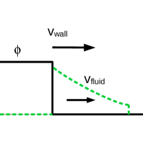
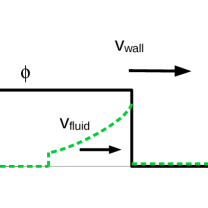
Figure 1: Deflagration (left) and detonation (right). In deflagration $v_{\rm wall}<v_{\rm sound}$, and the growing bubble wall pushes the fluid in front of it. In detonation $v_{\rm wall}>v_{\rm sound}$, and the bubble wall drags the fluid behind it.

In Figure 2 we show three snapshots of fluid kinetic energy density from a simulation at $\eta=0.15$, taken at the bubble growth stage, collision stage and after the bubbles have vanished. During the growth stage the kinetic energy is concentrated near the growing bubble walls. After the bubbles have collided the bubble walls vanish, but the fluid flow continues propagating as spherical compression waves, i.e. sound.

     

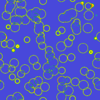
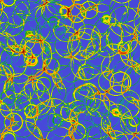
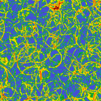
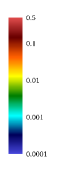
Figure 2: Fluid kinetic energy density at $t=500/T_{c}$, $1000/T_{c}$ and $1500/T_{c}$, at $\eta=0.15T_{c}$, corresponding to the growth phase of the bubbles, end of bubble collisions and after the bubbles have vanished. The shock waves caused by the bubbles remain for a long time after the transition has completed.

   

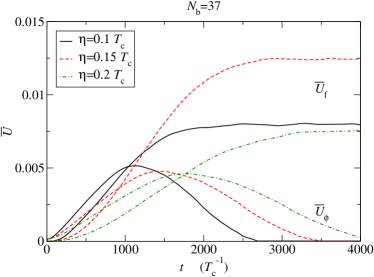
Figure 3: Left: the relative contribution from the field ($\bar{U}_{\phi}$) and fluid ($\bar{U}_{f}$) to the energy-momentum tensor. Right: the gravitational radiation power $\rho_{\rm gw}$ as a function of time.

The contribution of the field and fluid to the stress-energy tensor (and hence gravitational waves) can be quantified by introducing RMS fluid velocity $\bar{U}_{f}$ and the equivalent field quantity:

$$(\bar{\epsilon}+\bar{p})\bar{U}_{f}^{2}=\frac{1}{V}\int dV\tau_{ii}^{\rm fluid},~{}~{}~{}~{}~{}~{}~{}~{}~{}~{}(\bar{\epsilon}+\bar{p})\bar{U}_{\phi}^{2}=\frac{1}{V}\int dV\tau_{ii}^{\rm field}.$$ (9)

Here $\bar{\epsilon}$ and $\bar{p}$ are average energy density and pressure. In Figure 3 we see that the field and fluid contributions are comparable only during the bubble growth and collision stages. After the bubbles have collided, $\bar{U}_{\phi}\approx 0$ but the fluid kinetic energy remains approximately constant. This implies that the gravitational wave production also remains active for much longer than the transition time itself; indeed, it can be estimated to continue for up to Hubble time [26]. From Figure 3 we can also see that the gravitational wave power grows linearly with an universal slope:

$$\rho_{\rm GW}=t\,C\,GL_{f}(\bar{\epsilon}+\bar{p})^{2}\bar{U}_{f}^{4},~{}~{}~{}\mbox{with}~{}C=0.8\pm 0.2$$ (10)

Here $L_{f}$ is characteristic flow length scale. We can estimate that the total power is up to two orders of magnitude stronger than the estimate from the envelope approximation.

     

Figure 4: Gravitational wave power spectra from detonation (left) and deflagration (right). The development of characteristic power laws can be observed.

Finally, in Figure 4 we show an example of the development of the gravitational wave power spectra from detonation and deflagration. We see the development of characteristic power laws, with possibly non-universal power. For weak deflagration, we observe $\rho_{\rm GW}\propto k^{-3}$ on the UV end of the spectrum, deviating strongly from the prediction from the envelope approximation ($\rho\propto k^{-1}$).

4 Conclusions

We have studied the production of the gravitational waves in first order phase transitions in the early universe. We observe that the dominant source of the radiation is the sound of the transition, i.e. compression waves generated by the growing bubbles. These sound waves propagate through the universe long after the transition has completed. This strongly enhances the production of the gravitational waves, giving up to two orders of magnitude stronger signal than earlier eastimates. This enhances the possibility of observation of primordial gravitational waves in future gravitational wave detectors.

Acknowledgments

We have used the facilities at the Finnish Centre for Scientific Computing CSC, and the COSMOS Consortium supercomputer (within the DiRAC Facility jointly funded by STFC and the Large Facilities Capital Fund of BIS). KR acknowledges support from the Academy of Finland project 1134018; MH and SH from the Science and Technology Facilities Council (grant number ST/J000477/1). DJW is supported by the People Programme (Marie Skłodowska-Curie actions) of the European Union Seventh Framework Programme (FP7/2007-2013) under grant agreement number PIEF-GA-2013-629425.

References

- [1] LIGO Scientific Collaboration, G. M. Harry, Class.Quant.Grav. 27 (2010) 084006.
- [2] T. Accadia et al., Plans for the upgrade of the gravitational wave detector VIRGO: Advanced VIRGO, in Proceedings, 12th Marcel Grossmann Meeting on General Relativity, Paris, France, July 12-18, 2009. Vol. 1-3, pp. 1738–1742, 2009.
- [3] KAGRA Collaboration, K. Somiya, Class.Quant.Grav. 29 (2012) 124007, [arXiv:1111.7185].
- [4] eLISA Collaboration, P. A. Seoane et al., arXiv:1305.5720.
- [5] K. Kajantie, M. Laine, K. Rummukainen, and M. E. Shaposhnikov, Phys.Rev.Lett. 77 (1996) 2887–2890, [hep-ph/9605288].
- [6] M. Gurtler, E.-M. Ilgenfritz, and A. Schiller, Phys.Rev. D56 (1997) 3888–3895, [hep-lat/9704013].
- [7] F. Csikor, Z. Fodor, and J. Heitger, Phys.Rev.Lett. 82 (1999) 21–24, [hep-ph/9809291].
- [8] M. D’Onofrio and K. Rummukainen, arXiv:1508.07161.
- [9] M. S. Carena, M. Quiros, and C. Wagner, Phys.Lett. B380 (1996) 81–91, [hep-ph/9603420].
- [10] D. Delepine, J. Gerard, R. Gonzalez Felipe, and J. Weyers, Phys.Lett. B386 (1996) 183–188, [hep-ph/9604440].
- [11] M. Laine and K. Rummukainen, Nucl.Phys. B535 (1998) 423–457, [hep-lat/9804019].
- [12] C. Grojean, G. Servant, and J. D. Wells, Phys.Rev. D71 (2005) 036001, [hep-ph/0407019].
- [13] S. Huber and M. Schmidt, Nucl.Phys. B606 (2001) 183–230, [hep-ph/0003122].
- [14] S. J. Huber, T. Konstandin, T. Prokopec, and M. G. Schmidt, Nucl.Phys. B757 (2006) 172–196, [hep-ph/0606298].
- [15] G. Dorsch, S. Huber, and J. No, JHEP 1310 (2013) 029, [arXiv:1305.6610].
- [16] P. J. Steinhardt, Phys.Rev. D25 (1982) 2074.
- [17] H. Kurki-Suonio, Nucl.Phys. B255 (1985) 231.
- [18] K. Enqvist, J. Ignatius, K. Kajantie, and K. Rummukainen, Phys.Rev. D45 (1992) 3415–3428.
- [19] A. Kosowsky, M. S. Turner, and R. Watkins, Phys.Rev. D45 (1992) 4514–4535.
- [20] A. Kosowsky and M. S. Turner, Phys.Rev. D47 (1993) 4372–4391, [astro-ph/9211004].
- [21] M. Kamionkowski, A. Kosowsky, and M. S. Turner, Phys.Rev. D49 (1994) 2837–2851, [astro-ph/9310044].
- [22] S. J. Huber and T. Konstandin, JCAP 0809 (2008) 022, [arXiv:0806.1828].
- [23] C. Caprini, R. Durrer, T. Konstandin, and G. Servant, Phys.Rev. D79 (2009) 083519, [arXiv:0901.1661].
- [24] C. J. Hogan, MNRAS 218 (1986) 629–636.
- [25] M. Hindmarsh, S. J. Huber, K. Rummukainen, and D. J. Weir, Phys.Rev.Lett. 112 (2014) 041301, [arXiv:1304.2433].
- [26] M. Hindmarsh, S. J. Huber, K. Rummukainen, and D. J. Weir, arXiv:1504.03291.
- [27] J. Ignatius, K. Kajantie, H. Kurki-Suonio, and M. Laine, Phys.Rev. D49 (1994) 3854–3868, [astro-ph/9309059].
- [28] H. Kurki-Suonio and M. Laine, Phys.Rev. D54 (1996) 7163–7171, [hep-ph/9512202].
- [29] J. Garcia-Bellido, D. G. Figueroa, and A. Sastre, Phys.Rev. D77 (2008) 043517, [arXiv:0707.0839].
- [30] J. Wilson and G. Matthews, Relativistic Numerical Hydrodyamics. Cambridge University Press, Cambridge, 2003.
- [31] J. T. Giblin and J. B. Mertens, Phys.Rev. D90 (2014), no. 2 023532, [arXiv:1405.4005].