A hybrid LDG-HWENO scheme for KdV-type equations111The research was supported by NSFC grants 11328104 and 11571290.

Dongmi Luo222School of Mathematical Sciences and Fujian Provincial Key Laboratory of Mathematical Modeling and High-Performance Scientific Computing, Xiamen University, Xiamen, Fujian 361005, China. E-mail: luodongmi@126.com., Weizhang Huang333Department of Mathematics, University of Kansas, Lawrence, Kansas 66045, U.S.A. E-mail: whuang@ku.edu., and Jianxian Qiu444School of Mathematical Sciences and Fujian Provincial Key Laboratory of Mathematical Modeling and High-Performance Scientific Computing, Xiamen University, Xiamen, Fujian 361005, China. E-mail: jxqiu@xmu.edu.cn.

Abstract

A hybrid LDG-HWENO scheme is proposed for the numerical solution of KdV-type partial differential equations. It evolves the cell averages of the physical solution and its moments (a feature of Hermite WENO) while discretizes high order spatial derivatives using the local DG method. The new scheme has the advantages of both LDG and HWENO methods, including the ability to deal with high order spatial derivatives and the use of a small number of global unknown variables. The latter is independent of the order of the scheme and the spatial order of the underlying differential equations. One and two dimensional numerical examples are presented to show that the scheme can attain the same formal high order accuracy as the LDG method.

Keywords: local discontinuous Galerkin method; third order equations; high order method; HWENO; KdV equation.

AMS(MOS) subject classification: 65M60, 35L65

1 Introduction

We consider the numerical solution of KdV-type equations in one and two spatial dimensions. The local discontinuous Galerkin (LDG) method for this type of partial differential equations (PDEs) has been studied in [25, 27]. The LDG method is an extension of the discontinuous Galerkin (DG) method aimed at solving PDEs containing higher than first order spatial derivatives. The DG method was first introduced by Reed and Hill [19] for solving linear hyperbolic problems for neutron transfer. A major development of the DG method was carried out by Cockburn et al. in a series of papers [2, 3, 4, 5].

The basic idea of the LDG method is to rewrite a PDE with high order spatial derivatives into a system of first order PDEs and then discretize it by the DG method. It can achieve nonlinear stability without slope limiters when carefully designed. The sub-optimal error estimates in L2superscript𝐿2L^{2} norm were obtained for the smooth solution of linear equations and the cell entropy inequality was proven in [27]. While the LDG method also has many other advantages, it has the disadvantage of employing a large number of unknown variables and the number increases rapidly as the order of the method increases especially in multiple dimensions and for high order PDEs. On the other hand, the essentially non-oscillatory (ENO) schemes of Shu and Osher [22, 23], the weighted ENO (WENO) schemes of Liu et al. [14] and Jiang and Shu [11], and Hermite WENO (HWENO) schemes of Qiu and Shu [17, 18] have the advantage of employing a small number of unknown variables. But they have the disadvantage that the stencil used in reconstruction is becoming wider with an increasing order of accuracy.

To avoid the disadvantages of DG/LDG and WENO schemes, based on the reconstruction procedure for HWENO limiter by Qiu and Shu [17, 18] a hybrid RKDG-HWENO scheme was proposed by Balsara et al. [1] for hyperbolic conservation laws. It has intrinsic robustness and smaller stencils of the RKDG scheme and takes the advantage of the WENO scheme with a small number of unknown variables. The scheme evolves lower moments while reconstructing the higher moments of the solution. Dumbser et al. [8] extended the scheme to a new family of in-cell recovery DG method, referred to as PN​PMsubscript𝑃𝑁subscript𝑃𝑀P_{N}P_{M} methods, where PNsubscript𝑃𝑁P_{N} indicates that a piecewise polynomial of degree N𝑁N is used to represent a DG solution, and PMsubscript𝑃𝑀P_{M} stands for a reconstructed polynomial solution of degree M𝑀M (Mβ‰₯N𝑀𝑁M\geq N) that is used to compute the numerical fluxes. This approach yields a general, unified framework that contains two important special cases, classical high order finite volume (FV) schemes (N=0)𝑁0(N=0) and the conventional discontinuous Galerkin (DG) method (N=M)𝑁𝑀(N=M), and has been applied successfully to simulate the Euler equations of compressible gas dynamics and the equations of ideal magnetohydrodynamics (MHD). PN​PMsubscript𝑃𝑁subscript𝑃𝑀P_{N}P_{M} methods were extended to the numerical solution of the compressible Navier-Stokes equations [7, 15].

Motivated by the hybrid RKDG-HWENO and PN​PMsubscript𝑃𝑁subscript𝑃𝑀P_{N}P_{M} methods, we propose a hybrid LDG-HWENO scheme for the numerical solution of KdV-type PDEs. To our best knowledge, those methods have not been studied for higher order PDEs like KdV-type equations containing third order spatial derivatives. The new scheme employs LDG to approximate higher than first order spatial derivatives contained in the PDEs. Also different from HWENO methods in [17, 18], where the cell averages of both the solution u𝑒u and its first derivative uxsubscript𝑒π‘₯u_{x} are evolved in time and used in the reconstruction, we use the cell averages of u𝑒u (the solution) and u​xβˆ’xjΔ​x𝑒π‘₯subscriptπ‘₯𝑗Δπ‘₯u\frac{x-x_{j}}{\Delta x} (the first moment(s)) which are used in the reconstruction procedure for HWENO limiter [17, 18]. The new scheme employs only a small number of (global) unknown variables and uses a small stencil in the reconstruction. Numerical examples show that the new scheme can attain the same formal high order accuracy as the LDG method.

An outline of the paper is given as follows. The hybrid LDG-HWENO scheme is described in Sections 2 and 3 for one and two dimensional KdV-type equations, respectively. In Section 4, a selection of one and two dimensional numerical examples are presented to demonstrate the accuracy and the capability of the scheme. Conclusions are drawn in Section 5.

2 The hybrid LDG-HWENO scheme in one dimension

We consider the numerical solution of one dimensional KdV-type problems in the general form,

ut+f​(u)x+(r′​(u)​g​(r​(u)x)x)x=0,a<x<b,t>0formulae-sequenceformulae-sequencesubscript𝑒𝑑𝑓subscript𝑒π‘₯subscriptsuperscriptπ‘Ÿβ€²π‘’π‘”subscriptπ‘Ÿsubscript𝑒π‘₯π‘₯π‘₯0π‘Žπ‘₯𝑏𝑑0u_{t}+f(u)_{x}+(r^{\prime}(u)g(r(u)_{x})_{x})_{x}=0,\quad a<x<b,\;t>0 (2.1)

with the initial condition

u​(x,0)=u0​(x),a≀x≀bformulae-sequence𝑒π‘₯0subscript𝑒0π‘₯π‘Žπ‘₯𝑏u(x,0)=u_{0}(x),\quad a\leq x\leq b

where f​(u),r​(u)π‘“π‘’π‘Ÿπ‘’f(u),r(u), and g​(r)π‘”π‘Ÿg(r) are given smooth functions. In this work, we consider a uniform mesh of cell size Δ​xΞ”π‘₯\Delta x. Denote the cells by Ij=(xjβˆ’12,xj+12)subscript𝐼𝑗subscriptπ‘₯𝑗12subscriptπ‘₯𝑗12I_{j}=(x_{j-\frac{1}{2}},x_{j+\frac{1}{2}}), where xj+12=12​(xj+xj+1)subscriptπ‘₯𝑗1212subscriptπ‘₯𝑗subscriptπ‘₯𝑗1x_{j+\frac{1}{2}}=\frac{1}{2}(x_{j}+x_{j+1}). As for the HWENO scheme [17, 18], we want to find the approximations for the cell averages of u𝑒u and u​xβˆ’xjΔ​x𝑒π‘₯subscriptπ‘₯𝑗Δπ‘₯u\frac{x-x_{j}}{\Delta x} of the solution of (2.1), i.e.,

uΒ―jβ‰ˆ1Δ​xβ€‹βˆ«Iju​𝑑x,vΒ―jβ‰ˆ1Δ​xβ€‹βˆ«Iju​xβˆ’xjΔ​x​𝑑x.formulae-sequencesubscript¯𝑒𝑗1Ξ”π‘₯subscriptsubscript𝐼𝑗𝑒differential-dπ‘₯subscript¯𝑣𝑗1Ξ”π‘₯subscriptsubscript𝐼𝑗𝑒π‘₯subscriptπ‘₯𝑗Δπ‘₯differential-dπ‘₯\bar{u}_{j}\approx\frac{1}{\Delta x}\int_{I_{j}}udx,\quad\bar{v}_{j}\approx\frac{1}{\Delta x}\int_{I_{j}}u\frac{x-x_{j}}{\Delta x}dx.

Similar to the procedure of HWENO limiter for DG in [17, 18], we use here the first moment vΒ―jsubscript¯𝑣𝑗\bar{v}_{j} instead of the cell average of uxsubscript𝑒π‘₯u_{x} which was used for HWENO scheme in [17, 18]. This is more consistent with the basis functions of LDG (see (2.5) below). We employ LDG (e.g., see [25, 27]) for the discretization of high order spatial derivatives in (2.1). We first introduce the new variables

q=r​(u)x,p=g​(q)x,formulae-sequenceπ‘žπ‘Ÿsubscript𝑒π‘₯𝑝𝑔subscriptπ‘žπ‘₯q=r(u)_{x},\qquad p=g(q)_{x},

and rewrite (2.1) as a system of first order differential equations,

ut+(f​(u)+r′​(u)​p)xsubscript𝑒𝑑subscript𝑓𝑒superscriptπ‘Ÿβ€²π‘’π‘π‘₯\displaystyle u_{t}+(f(u)+r^{\prime}(u)p)_{x} =0,absent0\displaystyle=0, (2.2)
p𝑝\displaystyle p =g​(q)x,absent𝑔subscriptπ‘žπ‘₯\displaystyle=g(q)_{x}, (2.3)
qπ‘ž\displaystyle q =r​(u)x.absentπ‘Ÿsubscript𝑒π‘₯\displaystyle=r(u)_{x}. (2.4)

Next, we consider the discretization of (2.3) and (2.4). Let p𝑝p and qπ‘žq be approximated by

ph=βˆ‘l=0kpj(l)​ϕl(j)​(x),qh=βˆ‘l=0kqj(l)​ϕl(j)​(x),βˆ€x∈Ijformulae-sequencesubscriptπ‘β„Žsubscriptsuperscriptπ‘˜π‘™0subscriptsuperscript𝑝𝑙𝑗subscriptsuperscriptitalic-ϕ𝑗𝑙π‘₯formulae-sequencesubscriptπ‘žβ„Žsubscriptsuperscriptπ‘˜π‘™0subscriptsuperscriptπ‘žπ‘™π‘—subscriptsuperscriptitalic-ϕ𝑗𝑙π‘₯for-allπ‘₯subscript𝐼𝑗p_{h}=\sum\limits^{k}_{l=0}p^{(l)}_{j}\phi^{(j)}_{l}(x),\quad q_{h}=\sum\limits^{k}_{l=0}q^{(l)}_{j}\phi^{(j)}_{l}(x),\quad\forall x\in I_{j}

where Ο•l(j)​(x)subscriptsuperscriptitalic-ϕ𝑗𝑙π‘₯\phi^{(j)}_{l}(x)’s are the orthogonal basis functions and kπ‘˜k is the highest degree of polynomials used in the basis functions. The first five basis functions are

Ο•0(j)​(x)=1,subscriptsuperscriptitalic-ϕ𝑗0π‘₯1\displaystyle\phi^{(j)}_{0}(x)=1, Ο•1(j)​(x)=xβˆ’xjΔ​x,subscriptsuperscriptitalic-ϕ𝑗1π‘₯π‘₯subscriptπ‘₯𝑗Δπ‘₯\displaystyle\phi^{(j)}_{1}(x)=\frac{x-x_{j}}{\Delta x}, (2.5)
Ο•2(j)​(x)=(xβˆ’xjΔ​x)2βˆ’112,subscriptsuperscriptitalic-ϕ𝑗2π‘₯superscriptπ‘₯subscriptπ‘₯𝑗Δπ‘₯2112\displaystyle\phi^{(j)}_{2}(x)=(\frac{x-x_{j}}{\Delta x})^{2}-\frac{1}{12}, Ο•3(j)​(x)=(xβˆ’xjΔ​x)3βˆ’320​xβˆ’xjΔ​x,subscriptsuperscriptitalic-ϕ𝑗3π‘₯superscriptπ‘₯subscriptπ‘₯𝑗Δπ‘₯3320π‘₯subscriptπ‘₯𝑗Δπ‘₯\displaystyle\phi^{(j)}_{3}(x)=(\frac{x-x_{j}}{\Delta x})^{3}-\frac{3}{20}\frac{x-x_{j}}{\Delta x},
Ο•4(j)​(x)=(xβˆ’xjΔ​x)4βˆ’314​(xβˆ’xjΔ​x)2+3560.subscriptsuperscriptitalic-ϕ𝑗4π‘₯superscriptπ‘₯subscriptπ‘₯𝑗Δπ‘₯4314superscriptπ‘₯subscriptπ‘₯𝑗Δπ‘₯23560\displaystyle\phi^{(j)}_{4}(x)=(\frac{x-x_{j}}{\Delta x})^{4}-\frac{3}{14}(\frac{x-x_{j}}{\Delta x})^{2}+\frac{3}{560}.

Multiplying (2.3) and (2.4) by test functions w𝑀w and z𝑧z, respectively, integrating over the interval Ijsubscript𝐼𝑗I_{j}, integrating by parts, and replacing function values at cell boundaries by their numerical fluxes (those quantities with β€œhats”) which we will define in the below, we obtain

∫Ijph​w​𝑑x+∫Ijg​(qh)​wx​𝑑xβˆ’g^j+12​wj+12βˆ’+g^jβˆ’12​wjβˆ’12+=0,subscriptsubscript𝐼𝑗subscriptπ‘β„Žπ‘€differential-dπ‘₯subscriptsubscript𝐼𝑗𝑔subscriptπ‘žβ„Žsubscript𝑀π‘₯differential-dπ‘₯subscript^𝑔𝑗12subscriptsuperscript𝑀𝑗12subscript^𝑔𝑗12subscriptsuperscript𝑀𝑗120\displaystyle\int_{I_{j}}p_{h}wdx+\int_{I_{j}}g(q_{h})w_{x}dx-\hat{g}_{j+\frac{1}{2}}w^{-}_{j+\frac{1}{2}}+\hat{g}_{j-\frac{1}{2}}w^{+}_{j-\frac{1}{2}}=0, (2.6)
∫Ijqh​z​𝑑x+∫Ijr​(u)​zx​𝑑xβˆ’r^j+12​zj+12βˆ’+r^jβˆ’12​zjβˆ’12+=0,subscriptsubscript𝐼𝑗subscriptπ‘žβ„Žπ‘§differential-dπ‘₯subscriptsubscriptπΌπ‘—π‘Ÿπ‘’subscript𝑧π‘₯differential-dπ‘₯subscript^π‘Ÿπ‘—12subscriptsuperscript𝑧𝑗12subscript^π‘Ÿπ‘—12subscriptsuperscript𝑧𝑗120\displaystyle\int_{I_{j}}q_{h}zdx+\int_{I_{j}}r(u)z_{x}dx-\hat{r}_{j+\frac{1}{2}}z^{-}_{j+\frac{1}{2}}+\hat{r}_{j-\frac{1}{2}}z^{+}_{j-\frac{1}{2}}=0, (2.7)

where

wjΒ±12Β±=limxβ†’xjΒ±12Β±0w​(x),zjΒ±12Β±=limxβ†’xjΒ±12Β±0z​(x).formulae-sequencesuperscriptsubscript𝑀plus-or-minus𝑗12plus-or-minussubscriptβ†’π‘₯plus-or-minussubscriptπ‘₯plus-or-minus𝑗120𝑀π‘₯superscriptsubscript𝑧plus-or-minus𝑗12plus-or-minussubscriptβ†’π‘₯plus-or-minussubscriptπ‘₯plus-or-minus𝑗120𝑧π‘₯w_{j\pm\frac{1}{2}}^{\pm}=\lim_{x\to x_{j\pm\frac{1}{2}}\pm 0}w(x),\quad z_{j\pm\frac{1}{2}}^{\pm}=\lim_{x\to x_{j\pm\frac{1}{2}}\pm 0}z(x).

The test functions w𝑀w and z𝑧z in (2.6) and (2.7) are taken as the basis functions Ο•l(j)​(x),l=0,1,β‹―,kformulae-sequencesubscriptsuperscriptitalic-ϕ𝑗𝑙π‘₯𝑙01β‹―π‘˜\phi^{(j)}_{l}(x),\quad l=0,1,\cdots,k, successively. The integrals in (2.6) and (2.7) are computed numerically using a Gaussian quadrature rule. For the (k+1π‘˜1k+1)th order accuracy, the integration must achieve (2​k+2)2π‘˜2(2k+2)th order as the DG method. Thus, we use the (k+1)βˆ’limit-fromπ‘˜1(k+1)-point Gaussian quadrature, namely,

∫Ijg​(qh)​wx​𝑑xβ‰ˆΞ”β€‹xβ€‹βˆ‘Gg​(qh​(xG))​wx​(xG)​wG,subscriptsubscript𝐼𝑗𝑔subscriptπ‘žβ„Žsubscript𝑀π‘₯differential-dπ‘₯Ξ”π‘₯subscript𝐺𝑔subscriptπ‘žβ„Žsubscriptπ‘₯𝐺subscript𝑀π‘₯subscriptπ‘₯𝐺subscript𝑀𝐺\int_{I_{j}}g(q_{h})w_{x}dx\approx\Delta x\sum_{G}g(q_{h}(x_{G}))w_{x}(x_{G})w_{G},
∫Ijr​(u)​zx​𝑑xβ‰ˆΞ”β€‹xβ€‹βˆ‘Gr​(u​(xG))​zx​(xG)​wG,subscriptsubscriptπΌπ‘—π‘Ÿπ‘’subscript𝑧π‘₯differential-dπ‘₯Ξ”π‘₯subscriptπΊπ‘Ÿπ‘’subscriptπ‘₯𝐺subscript𝑧π‘₯subscriptπ‘₯𝐺subscript𝑀𝐺\int_{I_{j}}r(u)z_{x}dx\approx\Delta x\sum_{G}r(u(x_{G}))z_{x}(x_{G})w_{G},

where wGsubscript𝑀𝐺w_{G}’s are the weights and xGsubscriptπ‘₯𝐺x_{G}’s are the Gauss points. The function qhsubscriptπ‘žβ„Žq_{h} used in the first integral is obtained by solving (2.7) while the value u​(xG)𝑒subscriptπ‘₯𝐺u(x_{G}) used in the second integral is reconstructed from the cell averages {uΒ―j,vΒ―jsubscript¯𝑒𝑗subscript¯𝑣𝑗\bar{u}_{j},\bar{v}_{j}}. For example, the sixth order reconstruction procedure includes following five steps.

Step 1. Define the small stencils

S0={Ijβˆ’1,Ij,Ijβˆ’1β€²,Ijβ€²},S1={Ij,Ij+1,Ijβ€²,Ij+1β€²},S2={Ijβˆ’1,Ij,Ij+1,Ijβ€²}formulae-sequencesubscript𝑆0subscript𝐼𝑗1subscript𝐼𝑗subscriptsuperscript𝐼′𝑗1subscriptsuperscript𝐼′𝑗formulae-sequencesubscript𝑆1subscript𝐼𝑗subscript𝐼𝑗1subscriptsuperscript𝐼′𝑗subscriptsuperscript𝐼′𝑗1subscript𝑆2subscript𝐼𝑗1subscript𝐼𝑗subscript𝐼𝑗1subscriptsuperscript𝐼′𝑗S_{0}=\{I_{j-1},I_{j},I^{\prime}_{j-1},I^{\prime}_{j}\},\quad S_{1}=\{I_{j},I_{j+1},I^{\prime}_{j},I^{\prime}_{j+1}\},\quad S_{2}=\{I_{j-1},I_{j},I_{j+1},I^{\prime}_{j}\}

and a bigger stencil S={S0,S1,S2}𝑆subscript𝑆0subscript𝑆1subscript𝑆2S=\{S_{0},S_{1},S_{2}\}, where Ijsubscript𝐼𝑗I_{j} and Ijβ€²superscriptsubscript𝐼𝑗′I_{j}^{\prime} stand for intervals chosen for uΒ―jsubscript¯𝑒𝑗\bar{u}_{j} and vΒ―jsubscript¯𝑣𝑗\bar{v}_{j}, respectively. These stencils are used to construct polynomials p0​(x)subscript𝑝0π‘₯p_{0}(x), p1​(x)subscript𝑝1π‘₯p_{1}(x), and p2​(x)subscript𝑝2π‘₯p_{2}(x) of degree three and polynomial Q​(x)𝑄π‘₯Q(x) of degree five,

1Δ​xβ€‹βˆ«Ij+lp0​(x)​𝑑x=uΒ―j+l,1Δ​xβ€‹βˆ«Ij+lβ€²=Ij+lp0​(x)​xβˆ’xjΔ​x​𝑑x=vΒ―j+l,l=βˆ’1,0formulae-sequence1Ξ”π‘₯subscriptsubscript𝐼𝑗𝑙subscript𝑝0π‘₯differential-dπ‘₯subscript¯𝑒𝑗𝑙formulae-sequence1Ξ”π‘₯subscriptsubscriptsuperscript𝐼′𝑗𝑙subscript𝐼𝑗𝑙subscript𝑝0π‘₯π‘₯subscriptπ‘₯𝑗Δπ‘₯differential-dπ‘₯subscript¯𝑣𝑗𝑙𝑙10\displaystyle\frac{1}{\Delta x}\int_{I_{j+l}}p_{0}(x)dx=\bar{u}_{j+l},\quad\frac{1}{\Delta x}\int_{I^{\prime}_{j+l}=I_{j+l}}p_{0}(x)\frac{x-x_{j}}{\Delta x}dx=\bar{v}_{j+l},\quad l=-1,0
1Δ​xβ€‹βˆ«Ij+lp1​(x)​𝑑x=uΒ―j+l,1Δ​xβ€‹βˆ«Ij+lβ€²=Ij+lp1​(x)​xβˆ’xjΔ​x​𝑑x=vΒ―j+l,l=0,1formulae-sequence1Ξ”π‘₯subscriptsubscript𝐼𝑗𝑙subscript𝑝1π‘₯differential-dπ‘₯subscript¯𝑒𝑗𝑙formulae-sequence1Ξ”π‘₯subscriptsubscriptsuperscript𝐼′𝑗𝑙subscript𝐼𝑗𝑙subscript𝑝1π‘₯π‘₯subscriptπ‘₯𝑗Δπ‘₯differential-dπ‘₯subscript¯𝑣𝑗𝑙𝑙01\displaystyle\frac{1}{\Delta x}\int_{I_{j+l}}p_{1}(x)dx=\bar{u}_{j+l},\quad\frac{1}{\Delta x}\int_{I^{\prime}_{j+l}=I_{j+l}}p_{1}(x)\frac{x-x_{j}}{\Delta x}dx=\bar{v}_{j+l},\quad l=0,1
1Δ​xβ€‹βˆ«Ij+lp2​(x)​𝑑x=uΒ―j+l,1Δ​xβ€‹βˆ«Ijβ€²=Ijp2​(x)​xβˆ’xjΔ​x​𝑑x=vΒ―j,l=βˆ’1,0,1formulae-sequence1Ξ”π‘₯subscriptsubscript𝐼𝑗𝑙subscript𝑝2π‘₯differential-dπ‘₯subscript¯𝑒𝑗𝑙formulae-sequence1Ξ”π‘₯subscriptsubscriptsuperscript𝐼′𝑗subscript𝐼𝑗subscript𝑝2π‘₯π‘₯subscriptπ‘₯𝑗Δπ‘₯differential-dπ‘₯subscript¯𝑣𝑗𝑙101\displaystyle\frac{1}{\Delta x}\int_{I_{j+l}}p_{2}(x)dx=\bar{u}_{j+l},\quad\frac{1}{\Delta x}\int_{I^{\prime}_{j}=I_{j}}p_{2}(x)\frac{x-x_{j}}{\Delta x}dx=\bar{v}_{j},\quad l=-1,0,1
1Δ​xβ€‹βˆ«Ij+lQ​(x)​𝑑x=uΒ―j+l,1Δ​xβ€‹βˆ«Ij+lβ€²=Ij+lQ​(x)​xβˆ’xjΔ​x​𝑑x=vΒ―j+l,l=βˆ’1,0,1.formulae-sequence1Ξ”π‘₯subscriptsubscript𝐼𝑗𝑙𝑄π‘₯differential-dπ‘₯subscript¯𝑒𝑗𝑙formulae-sequence1Ξ”π‘₯subscriptsubscriptsuperscript𝐼′𝑗𝑙subscript𝐼𝑗𝑙𝑄π‘₯π‘₯subscriptπ‘₯𝑗Δπ‘₯differential-dπ‘₯subscript¯𝑣𝑗𝑙𝑙101\displaystyle\frac{1}{\Delta x}\int_{I_{j+l}}Q(x)dx=\bar{u}_{j+l},\quad\frac{1}{\Delta x}\int_{I^{\prime}_{j+l}=I_{j+l}}Q(x)\frac{x-x_{j}}{\Delta x}dx=\bar{v}_{j+l},\quad l=-1,0,1.

Step 2. Compute the smoothness indicators, denoted by Ξ²lsubscript𝛽𝑙\beta_{l} for each stencil Slsubscript𝑆𝑙S_{l}. They measure how smooth p0​(x),p1​(x)subscript𝑝0π‘₯subscript𝑝1π‘₯p_{0}(x),\;p_{1}(x), and p2​(x)subscript𝑝2π‘₯p_{2}(x) are in the target cell Ijsubscript𝐼𝑗I_{j}. Following [11], we define

Ξ²l=βˆ‘m=13∫IjΔ​x2​mβˆ’1​(dm​pl​(x)d​xm)2​𝑑x,l=0,1,2.formulae-sequencesubscript𝛽𝑙subscriptsuperscript3π‘š1subscriptsubscript𝐼𝑗Δsuperscriptπ‘₯2π‘š1superscriptsuperscriptπ‘‘π‘šsubscript𝑝𝑙π‘₯𝑑superscriptπ‘₯π‘š2differential-dπ‘₯𝑙012\beta_{l}=\sum\limits^{3}_{m=1}\int_{I_{j}}\Delta x^{2m-1}(\frac{d^{m}p_{l}(x)}{dx^{m}})^{2}dx,\quad l=0,1,2.

Step 3. For a given point x^∈Ij^π‘₯subscript𝐼𝑗\hat{x}\in I_{j}, we find the linear weights, denoted by Ξ³0,Ξ³1subscript𝛾0subscript𝛾1\gamma_{0},\gamma_{1} and Ξ³2subscript𝛾2\gamma_{2}, such that

Q​(x^)=βˆ‘i=02Ξ³i​pi​(x^).𝑄^π‘₯subscriptsuperscript2𝑖0subscript𝛾𝑖subscript𝑝𝑖^π‘₯Q(\hat{x})=\sum\limits^{2}_{i=0}\gamma_{i}p_{i}(\hat{x}).

For example, for x^=xj+12^π‘₯subscriptπ‘₯𝑗12\hat{x}=x_{j+\frac{1}{2}} we have

Ξ³0=25189,Ξ³1=1427,Ξ³2=2263.formulae-sequencesubscript𝛾025189formulae-sequencesubscript𝛾11427subscript𝛾22263\gamma_{0}=\frac{25}{189},\quad\gamma_{1}=\frac{14}{27},\quad\gamma_{2}=\frac{22}{63}.

Step 4. The nonlinear weights based on the smoothness indicators are computed as

Ο‰m=ω¯mβˆ‘l=02ω¯l,ω¯l=Ξ³l(Ξ»+Ξ²l)2,m=0,1,2,formulae-sequencesubscriptπœ”π‘šsubscriptΒ―πœ”π‘šsuperscriptsubscript𝑙02subscriptΒ―πœ”π‘™formulae-sequencesubscriptΒ―πœ”π‘™subscript𝛾𝑙superscriptπœ†subscript𝛽𝑙2π‘š012\omega_{m}=\frac{\bar{\omega}_{m}}{\sum\limits_{l=0}^{2}\bar{\omega}_{l}},\quad\bar{\omega}_{l}=\frac{\gamma_{l}}{(\lambda+\beta_{l})^{2}},\quad m=0,1,2,

where Ξ»πœ†\lambda is a small positive number to avoid the denominator to become zero.

Step 5. Finally, the HWENO reconstruction is given by

u​(x^)=βˆ‘i=02Ο‰i​pi​(x^).𝑒^π‘₯subscriptsuperscript2𝑖0subscriptπœ”π‘–subscript𝑝𝑖^π‘₯u(\hat{x})=\sum\limits^{2}_{i=0}\omega_{i}p_{i}(\hat{x}). (2.8)

Step 3 to Step 5 are repeated for each point x^∈{{xG},xjβˆ’12,xj+12}^π‘₯subscriptπ‘₯𝐺subscriptπ‘₯𝑗12subscriptπ‘₯𝑗12\hat{x}\in\{\{x_{G}\},x_{j-\frac{1}{2}},x_{j+\frac{1}{2}}\}, where {xG}subscriptπ‘₯𝐺\{x_{G}\} denotes the set of the Gauss points.

It is remarked that the reconstructed values of u𝑒u at both ends of Ijsubscript𝐼𝑗I_{j} are denoted by ujβˆ’12+subscriptsuperscript𝑒𝑗12u^{+}_{j-\frac{1}{2}} and uj+12βˆ’subscriptsuperscript𝑒𝑗12u^{-}_{j+\frac{1}{2}}, respectively. Moreover, the linear weights for some points can become negative. For example, for xG=xjβˆ’0.53846931010568312subscriptπ‘₯𝐺subscriptπ‘₯𝑗0.53846931010568312x_{G}=x_{j-\frac{0.5384693101056831}{2}}, the linear weights are Ξ³0=βˆ’1.19876833424689subscript𝛾01.19876833424689\gamma_{0}=-1.19876833424689, Ξ³1=βˆ’0.189130224626382subscript𝛾10.189130224626382\gamma_{1}=-0.189130224626382, and Ξ³2=2.38789855887328subscript𝛾22.38789855887328\gamma_{2}=2.38789855887328. The negative weights may lead to instability of the reconstruction. The technique developed by Shi et al. [20] can be used to treat reconstruction procedure with negative weights; the interested reader is referred to [20] for the detail.

Multiplying (2.2) with 111 and xβˆ’xjΔ​xπ‘₯subscriptπ‘₯𝑗Δπ‘₯\frac{x-x_{j}}{\Delta x} and integrating them by parts over Ijsubscript𝐼𝑗I_{j}, we have

d​uΒ―jd​t=βˆ’1Δ​x​(f​(u)+r′​(u)​p)|Ij,𝑑subscript¯𝑒𝑗𝑑𝑑evaluated-at1Ξ”π‘₯𝑓𝑒superscriptπ‘Ÿβ€²π‘’π‘subscript𝐼𝑗\displaystyle\frac{d\bar{u}_{j}}{dt}=-\frac{1}{\Delta x}(f(u)+r^{\prime}(u)p)|_{I_{j}}, (2.9)
d​vΒ―jd​t=βˆ’1Δ​x​(f​(u)+r′​(u)​p)​xβˆ’xjΔ​x|Ij+1Δ​x2β€‹βˆ«Ij(f​(u)+r′​(u)​p)​𝑑x.𝑑subscript¯𝑣𝑗𝑑𝑑evaluated-at1Ξ”π‘₯𝑓𝑒superscriptπ‘Ÿβ€²π‘’π‘π‘₯subscriptπ‘₯𝑗Δπ‘₯subscript𝐼𝑗1Ξ”superscriptπ‘₯2subscriptsubscript𝐼𝑗𝑓𝑒superscriptπ‘Ÿβ€²π‘’π‘differential-dπ‘₯\displaystyle\frac{d\bar{v}_{j}}{dt}=-\frac{1}{\Delta x}(f(u)+r^{\prime}(u)p)\frac{x-x_{j}}{\Delta x}|_{I_{j}}+\frac{1}{\Delta x^{2}}\int_{I_{j}}(f(u)+r^{\prime}(u)p)dx. (2.10)

The integral term in (2.10) is approximated by the (k+1)π‘˜1(k+1)-point Gaussian quadrature rule as for (2.6) and (2.7). We obtain the numerical scheme as

d​uΒ―jd​t=βˆ’1Δ​x​[(f^j+12+r^j+12′​p^j+12)βˆ’(f^jβˆ’12+r^jβˆ’12′​p^jβˆ’12)],𝑑subscript¯𝑒𝑗𝑑𝑑1Ξ”π‘₯delimited-[]subscript^𝑓𝑗12subscriptsuperscript^π‘Ÿβ€²π‘—12subscript^𝑝𝑗12subscript^𝑓𝑗12subscriptsuperscript^π‘Ÿβ€²π‘—12subscript^𝑝𝑗12\displaystyle\frac{d\bar{u}_{j}}{dt}=-\frac{1}{\Delta x}[(\hat{f}_{j+\frac{1}{2}}+\hat{r}^{\prime}_{j+\frac{1}{2}}\hat{p}_{j+\frac{1}{2}})-(\hat{f}_{j-\frac{1}{2}}+\hat{r}^{\prime}_{j-\frac{1}{2}}\hat{p}_{j-\frac{1}{2}})], (2.11)
d​vΒ―jd​t=βˆ’12​Δ​x​[(f^j+12+r^j+12′​p^j+12)+(f^jβˆ’12+r^jβˆ’12′​p^jβˆ’12)]+1Δ​x2​Fj,𝑑subscript¯𝑣𝑗𝑑𝑑12Ξ”π‘₯delimited-[]subscript^𝑓𝑗12subscriptsuperscript^π‘Ÿβ€²π‘—12subscript^𝑝𝑗12subscript^𝑓𝑗12subscriptsuperscript^π‘Ÿβ€²π‘—12subscript^𝑝𝑗121Ξ”superscriptπ‘₯2subscript𝐹𝑗\displaystyle\frac{d\bar{v}_{j}}{dt}=-\frac{1}{2\Delta x}[(\hat{f}_{j+\frac{1}{2}}+\hat{r}^{\prime}_{j+\frac{1}{2}}\hat{p}_{j+\frac{1}{2}})+(\hat{f}_{j-\frac{1}{2}}+\hat{r}^{\prime}_{j-\frac{1}{2}}\hat{p}_{j-\frac{1}{2}})]+\frac{1}{\Delta x^{2}}F_{j}, (2.12)

where

Fj=Δ​xβ€‹βˆ‘G(f​(u​(xG))+r′​(u​(xG))​ph​(xG))​wGβ‰ˆβˆ«Ij(f​(u)+r′​(u)​ph)​𝑑x.subscript𝐹𝑗Δπ‘₯subscript𝐺𝑓𝑒subscriptπ‘₯𝐺superscriptπ‘Ÿβ€²π‘’subscriptπ‘₯𝐺subscriptπ‘β„Žsubscriptπ‘₯𝐺subscript𝑀𝐺subscriptsubscript𝐼𝑗𝑓𝑒superscriptπ‘Ÿβ€²π‘’subscriptπ‘β„Ždifferential-dπ‘₯F_{j}=\Delta x\sum_{G}(f(u(x_{G}))+r^{\prime}(u(x_{G}))p_{h}(x_{G}))w_{G}\approx\int_{I_{j}}(f(u)+r^{\prime}(u)p_{h})dx.

A key component of the above described hybrid LDG-HWENO scheme is to define the numerical fluxes in (2.6), (2.7), (2.11), and (2.12) to ensure the accuracy and stability of the scheme. We define

f^j+12=f^​(uj+12βˆ’,uj+12+),subscript^𝑓𝑗12^𝑓subscriptsuperscript𝑒𝑗12subscriptsuperscript𝑒𝑗12\displaystyle\hat{f}_{j+\frac{1}{2}}=\hat{f}(u^{-}_{j+\frac{1}{2}},u^{+}_{j+\frac{1}{2}}), g^j+12=g^​(qj+12βˆ’,qj+12+),subscript^𝑔𝑗12^𝑔subscriptsuperscriptπ‘žπ‘—12subscriptsuperscriptπ‘žπ‘—12\displaystyle\hat{g}_{j+\frac{1}{2}}=\hat{g}(q^{-}_{j+\frac{1}{2}},q^{+}_{j+\frac{1}{2}}),
p^j+12=pj+12+,subscript^𝑝𝑗12subscriptsuperscript𝑝𝑗12\displaystyle\hat{p}_{j+\frac{1}{2}}=p^{+}_{j+\frac{1}{2}}, r^j+12=r​(uj+12βˆ’),subscript^π‘Ÿπ‘—12π‘Ÿsubscriptsuperscript𝑒𝑗12\displaystyle\hat{r}_{j+\frac{1}{2}}=r(u^{-}_{j+\frac{1}{2}}),
r^j+12β€²=r​(uj+12+)βˆ’r​(uj+12βˆ’)uj+12+βˆ’uj+12βˆ’,subscriptsuperscript^π‘Ÿβ€²π‘—12π‘Ÿsubscriptsuperscript𝑒𝑗12π‘Ÿsubscriptsuperscript𝑒𝑗12subscriptsuperscript𝑒𝑗12subscriptsuperscript𝑒𝑗12\displaystyle\hat{r}^{\prime}_{j+\frac{1}{2}}=\frac{r(u^{+}_{j+\frac{1}{2}})-r(u^{-}_{j+\frac{1}{2}})}{u^{+}_{j+\frac{1}{2}}-u^{-}_{j+\frac{1}{2}}},

where

pj+12Β±=ph​(xj+12Β±0),qj+12Β±=qh​(xj+12Β±0),formulae-sequencesuperscriptsubscript𝑝𝑗12plus-or-minussubscriptπ‘β„Žplus-or-minussubscriptπ‘₯𝑗120superscriptsubscriptπ‘žπ‘—12plus-or-minussubscriptπ‘žβ„Žplus-or-minussubscriptπ‘₯𝑗120p_{j+\frac{1}{2}}^{\pm}=p_{h}(x_{j+\frac{1}{2}}\pm 0),\quad q_{j+\frac{1}{2}}^{\pm}=q_{h}(x_{j+\frac{1}{2}}\pm 0),

and uj+12Β±superscriptsubscript𝑒𝑗12plus-or-minusu_{j+\frac{1}{2}}^{\pm} are the reconstructed values of u𝑒u by the HWENO method as described in StepΒ 1-StepΒ 5. It is noted that the choice of the numerical fluxes is not unique. The key part is that p^^𝑝\hat{p} and r^^π‘Ÿ\hat{r} must be taken from the opposite sides. The numerical flux f^​(a,b)^π‘“π‘Žπ‘\hat{f}(a,b) for f​(u)𝑓𝑒f(u) should satisfy the following conditions:

  1. (i)

    f^​(a,b)^π‘“π‘Žπ‘\hat{f}(a,b) is a Lipschitz continuous function in both arguments aπ‘Ža and b𝑏b;

  2. (ii)

    f^^𝑓\hat{f} is consistent with f​(u)𝑓𝑒f(u), namely, f^​(u,u)=f​(u)^𝑓𝑒𝑒𝑓𝑒\hat{f}(u,u)=f(u);

  3. (iii)

    f^​(a,b)^π‘“π‘Žπ‘\hat{f}(a,b) is a monotone flux, i.e., it is non-decreasing in aπ‘Ža and non-increasing in b𝑏b.

In this paper, we use the local Lax-Friedrichs(LLF) flux,

f^​(a,b)=12​[f​(a)+f​(b)βˆ’Ξ±β€‹(bβˆ’a)],Ξ±=maxu∈[min⁑(a,b),max⁑(a,b)]⁑|f′​(u)|.formulae-sequence^π‘“π‘Žπ‘12delimited-[]π‘“π‘Žπ‘“π‘π›Όπ‘π‘Žπ›Όsubscriptπ‘’π‘Žπ‘π‘Žπ‘superscript𝑓′𝑒\hat{f}(a,b)=\frac{1}{2}[f(a)+f(b)-\alpha(b-a)],\quad\alpha=\max\limits_{u\in[\min(a,b),\max(a,b)]}|f^{\prime}(u)|.

The numerical flux g^​(c,d)^𝑔𝑐𝑑\hat{g}(c,d) for g​(q)π‘”π‘žg(q) should also satisfy conditions (i) and (ii) but the condition (iii) should be replaced by

  1. (iii)’

    βˆ’g^​(qβˆ’,q+)^𝑔superscriptπ‘žsuperscriptπ‘ž-\hat{g}(q^{-},q^{+}) is a monotone flux for βˆ’g​(q)π‘”π‘ž-g(q), namely, g^​(c,d)^𝑔𝑐𝑑\hat{g}(c,d) is non-increasing in c𝑐c and non-decreasing in d𝑑d.

Corresponding to the LLF flux, we have

g^​(c,d)=12​[g​(c)+g​(d)βˆ’Ξ±β€‹(cβˆ’d)],Ξ±=maxq∈[min⁑(c,d),max⁑(c,d)]⁑|g′​(q)|.formulae-sequence^𝑔𝑐𝑑12delimited-[]𝑔𝑐𝑔𝑑𝛼𝑐𝑑𝛼subscriptπ‘žπ‘π‘‘π‘π‘‘superscriptπ‘”β€²π‘ž\hat{g}(c,d)=\frac{1}{2}[g(c)+g(d)-\alpha(c-d)],\quad\alpha=\max_{q\in[\min(c,d),\max(c,d)]}|g^{\prime}(q)|.

We note that (2.7) can be solved independently on each cell for qhsubscriptπ‘žβ„Žq_{h} in terms of the cell averages {uΒ―j,vΒ―j}subscript¯𝑒𝑗subscript¯𝑣𝑗\{\bar{u}_{j},\bar{v}_{j}\}. Similarly, (2.6) can be solved on each cell for phsubscriptπ‘β„Žp_{h} in terms of qhsubscriptπ‘žβ„Žq_{h}. As a consequence, the global unknown variables involve only uΒ―jsubscript¯𝑒𝑗\bar{u}_{j} and vΒ―jsubscript¯𝑣𝑗\bar{v}_{j}, which are governed by a system of ordinary differential equations. In our computation, the system is integrated in time using an explicit TVD Runge-Kutta method, such as the 3rd TVD Runge-Kutta method for solving

ut=L​(u,t),subscript𝑒𝑑𝐿𝑒𝑑u_{t}=L(u,t),

where L​(u,t)𝐿𝑒𝑑L(u,t) is a spatial discretization operator,

uβˆ—=un+Δ​t​L​(un,tn)superscript𝑒superscript𝑒𝑛Δ𝑑𝐿superscript𝑒𝑛superscript𝑑𝑛\displaystyle u^{*}=u^{n}+\Delta tL(u^{n},t^{n})
uβˆ—βˆ—=34​un+14​(uβˆ—+Δ​t​L​(uβˆ—,tn+Δ​t))superscript𝑒absent34superscript𝑒𝑛14superscript𝑒Δ𝑑𝐿superscript𝑒superscript𝑑𝑛Δ𝑑\displaystyle u^{**}=\frac{3}{4}u^{n}+\frac{1}{4}(u^{*}+\Delta tL(u^{*},t^{n}+\Delta t))
un+1=13​un+23​(uβˆ—βˆ—+Δ​t​L​(uβˆ—βˆ—,tn+12​Δ​t)).superscript𝑒𝑛113superscript𝑒𝑛23superscript𝑒absentΔ𝑑𝐿superscript𝑒absentsuperscript𝑑𝑛12Δ𝑑\displaystyle u^{n+1}=\frac{1}{3}u^{n}+\frac{2}{3}(u^{**}+\Delta tL(u^{**},t^{n}+\frac{1}{2}\Delta t)).

From the construction of the scheme, it is not difficult to show formally that the method is of (k+1)thsuperscriptπ‘˜1th(k+1)^{\text{th}} order in space (k≀4π‘˜4k\leq 4) and third order in time, i.e.,

ehn=π’ͺ​(Δ​t3)+π’ͺ​(Δ​xk+1).superscriptsubscriptπ‘’β„Žπ‘›π’ͺΞ”superscript𝑑3π’ͺΞ”superscriptπ‘₯π‘˜1e_{h}^{n}=\mathcal{O}(\Delta t^{3})+\mathcal{O}(\Delta x^{k+1}).

Since an explicit scheme is used, the time step is subject to the CFL condition and should be taken as Δ​t=π’ͺ​(Δ​x3)Δ𝑑π’ͺΞ”superscriptπ‘₯3\Delta t=\mathcal{O}(\Delta x^{3}). For this choice, the error is dominated by the spatial discretization error.

3 The hybrid LDG-HWENO method in two dimensions

In this section we describe the method for two dimensional problems. We consider the general form

ut+f1​(u)x+f2​(u)y+[r1′​(u)​(g11​(r1​(u)x)x+g12​(r1​(u)x)y)]xsubscript𝑒𝑑subscript𝑓1subscript𝑒π‘₯subscript𝑓2subscript𝑒𝑦subscriptdelimited-[]subscriptsuperscriptπ‘Ÿβ€²1𝑒subscript𝑔11subscriptsubscriptπ‘Ÿ1subscript𝑒π‘₯π‘₯subscript𝑔12subscriptsubscriptπ‘Ÿ1subscript𝑒π‘₯𝑦π‘₯\displaystyle u_{t}+f_{1}(u)_{x}+f_{2}(u)_{y}+[r^{\prime}_{1}(u)(g_{11}(r_{1}(u)_{x})_{x}+g_{12}(r_{1}(u)_{x})_{y})]_{x}
+[r2′​(u)​(g21​(r2​(u)y)x+g22​(r2​(u)y)y)]y=0,(x,y)∈(a,b)Γ—(c,d)formulae-sequencesubscriptdelimited-[]subscriptsuperscriptπ‘Ÿβ€²2𝑒subscript𝑔21subscriptsubscriptπ‘Ÿ2subscript𝑒𝑦π‘₯subscript𝑔22subscriptsubscriptπ‘Ÿ2subscript𝑒𝑦𝑦𝑦0π‘₯π‘¦π‘Žπ‘π‘π‘‘\displaystyle+[r^{\prime}_{2}(u)(g_{21}(r_{2}(u)_{y})_{x}+g_{22}(r_{2}(u)_{y})_{y})]_{y}=0,\quad(x,y)\in(a,b)\times(c,d) (3.1)

subject to a periodic boundary condition and the initial condition

u​(x,y,0)=u0​(x,y),(x,y)∈(a,b)Γ—(c,d)formulae-sequence𝑒π‘₯𝑦0subscript𝑒0π‘₯𝑦π‘₯π‘¦π‘Žπ‘π‘π‘‘u(x,y,0)=u_{0}(x,y),\quad(x,y)\in(a,b)\times(c,d)

where fm​(u)subscriptπ‘“π‘šπ‘’f_{m}(u), rm​(u)subscriptπ‘Ÿπ‘šπ‘’r_{m}(u), and gm​n​(r)subscriptπ‘”π‘šπ‘›π‘Ÿg_{mn}(r) are given smooth nonlinear functions.

We use a rectangle mesh of cell size Δ​xΞ”π‘₯\Delta x and Δ​yΔ𝑦\Delta y in xπ‘₯x and y𝑦y directions, respectively. We denote the cells by

Ii​j=(xiβˆ’12,xi+12)Γ—(yjβˆ’12,yj+12),subscript𝐼𝑖𝑗subscriptπ‘₯𝑖12subscriptπ‘₯𝑖12subscript𝑦𝑗12subscript𝑦𝑗12I_{ij}=(x_{i-\frac{1}{2}},\,x_{i+\frac{1}{2}})\times(y_{j-\frac{1}{2}},\,y_{j+\frac{1}{2}}),

where

xi+12=12​(xi+xi+1),yj+12=12​(yj+yj+1).formulae-sequencesubscriptπ‘₯𝑖1212subscriptπ‘₯𝑖subscriptπ‘₯𝑖1subscript𝑦𝑗1212subscript𝑦𝑗subscript𝑦𝑗1x_{i+\frac{1}{2}}=\frac{1}{2}(x_{i}+x_{i+1}),\quad y_{j+\frac{1}{2}}=\frac{1}{2}(y_{j}+y_{j+1}).

We approximate the cell averages of u𝑒u, u​xβˆ’xiΔ​x𝑒π‘₯subscriptπ‘₯𝑖Δπ‘₯u\frac{x-x_{i}}{\Delta x}, u​yβˆ’yjΔ​y𝑒𝑦subscript𝑦𝑗Δ𝑦u\frac{y-y_{j}}{\Delta y} and u​xβˆ’xiΔ​x​yβˆ’yjΔ​y𝑒π‘₯subscriptπ‘₯𝑖Δπ‘₯𝑦subscript𝑦𝑗Δ𝑦u\frac{x-x_{i}}{\Delta x}\frac{y-y_{j}}{\Delta y} by

uΒ―i​jβ‰ˆ1Δ​x​Δ​yβ€‹βˆ«Ii​ju​𝑑x​𝑑y,subscript¯𝑒𝑖𝑗1Ξ”π‘₯Δ𝑦subscriptsubscript𝐼𝑖𝑗𝑒differential-dπ‘₯differential-d𝑦\displaystyle\bar{u}_{ij}\approx\frac{1}{\Delta x\Delta y}\int_{I_{ij}}udxdy,
vΒ―i​jβ‰ˆ1Δ​x​Δ​yβ€‹βˆ«Ii​ju​xβˆ’xiΔ​x​𝑑x​𝑑y,subscript¯𝑣𝑖𝑗1Ξ”π‘₯Δ𝑦subscriptsubscript𝐼𝑖𝑗𝑒π‘₯subscriptπ‘₯𝑖Δπ‘₯differential-dπ‘₯differential-d𝑦\displaystyle\bar{v}_{ij}\approx\frac{1}{\Delta x\Delta y}\int_{I_{ij}}u\frac{x-x_{i}}{\Delta x}dxdy,
wΒ―i​jβ‰ˆ1Δ​x​Δ​yβ€‹βˆ«Ii​ju​yβˆ’yjΔ​y​𝑑x​𝑑y,subscript¯𝑀𝑖𝑗1Ξ”π‘₯Δ𝑦subscriptsubscript𝐼𝑖𝑗𝑒𝑦subscript𝑦𝑗Δ𝑦differential-dπ‘₯differential-d𝑦\displaystyle\bar{w}_{ij}\approx\frac{1}{\Delta x\Delta y}\int_{I_{ij}}u\frac{y-y_{j}}{\Delta y}dxdy,
ZΒ―i​jβ‰ˆ1Δ​x​Δ​yβ€‹βˆ«Ii​ju​xβˆ’xiΔ​x​yβˆ’yjΔ​y​𝑑x​𝑑y.subscript¯𝑍𝑖𝑗1Ξ”π‘₯Δ𝑦subscriptsubscript𝐼𝑖𝑗𝑒π‘₯subscriptπ‘₯𝑖Δπ‘₯𝑦subscript𝑦𝑗Δ𝑦differential-dπ‘₯differential-d𝑦\displaystyle\bar{Z}_{ij}\approx\frac{1}{\Delta x\Delta y}\int_{I_{ij}}u\frac{x-x_{i}}{\Delta x}\frac{y-y_{j}}{\Delta y}dxdy.

For the discretization of high order spatial derivatives using LDG, we introduce the new variables

q1=r1​(u)x,q2=r2​(u)y,p1=g11​(q1)x+g12​(q1)y,p2=g21​(q2)x+g22​(q2)y,formulae-sequencesubscriptπ‘ž1subscriptπ‘Ÿ1subscript𝑒π‘₯formulae-sequencesubscriptπ‘ž2subscriptπ‘Ÿ2subscript𝑒𝑦formulae-sequencesubscript𝑝1subscript𝑔11subscriptsubscriptπ‘ž1π‘₯subscript𝑔12subscriptsubscriptπ‘ž1𝑦subscript𝑝2subscript𝑔21subscriptsubscriptπ‘ž2π‘₯subscript𝑔22subscriptsubscriptπ‘ž2𝑦q_{1}=r_{1}(u)_{x},\quad q_{2}=r_{2}(u)_{y},\quad p_{1}=g_{11}(q_{1})_{x}+g_{12}(q_{1})_{y},\quad p_{2}=g_{21}(q_{2})_{x}+g_{22}(q_{2})_{y}, (3.2)

and rewrite (3.1) as a first order system

ut+(f1​(u)+r1′​(u)​p1)x+(f2​(u)+r2′​(u)​p2)y=0,subscript𝑒𝑑subscriptsubscript𝑓1𝑒subscriptsuperscriptπ‘Ÿβ€²1𝑒subscript𝑝1π‘₯subscriptsubscript𝑓2𝑒subscriptsuperscriptπ‘Ÿβ€²2𝑒subscript𝑝2𝑦0\displaystyle u_{t}+(f_{1}(u)+r^{\prime}_{1}(u)p_{1})_{x}+(f_{2}(u)+r^{\prime}_{2}(u)p_{2})_{y}=0, (3.3)

coupled with (3.2). We approximate pm,qm​(m=1,2)subscriptπ‘π‘šsubscriptπ‘žπ‘šπ‘š12p_{m},q_{m}(m=1,2) by polynomials,

pm=βˆ‘l=0kpm,l(i​j)​ϕl(i​j)​(x,y),qm=βˆ‘l=0kqm,l(i​j)​ϕl(i​j)​(x,y),m=1,2βˆ€(x,y)∈Ii​jformulae-sequencesubscriptπ‘π‘šsuperscriptsubscript𝑙0π‘˜superscriptsubscriptπ‘π‘šπ‘™π‘–π‘—subscriptsuperscriptitalic-ϕ𝑖𝑗𝑙π‘₯𝑦formulae-sequencesubscriptπ‘žπ‘šsuperscriptsubscript𝑙0π‘˜superscriptsubscriptπ‘žπ‘šπ‘™π‘–π‘—subscriptsuperscriptitalic-ϕ𝑖𝑗𝑙π‘₯𝑦formulae-sequenceπ‘š12for-allπ‘₯𝑦subscript𝐼𝑖𝑗p_{m}=\sum\limits_{l=0}^{k}p_{m,l}^{(ij)}\phi^{(ij)}_{l}(x,y),\quad q_{m}=\sum\limits_{l=0}^{k}q_{m,l}^{(ij)}\phi^{(ij)}_{l}(x,y),\quad m=1,2\quad\forall(x,y)\in I_{ij}

where Ο•l(i​j)​(x,y)subscriptsuperscriptitalic-ϕ𝑖𝑗𝑙π‘₯𝑦\phi^{(ij)}_{l}(x,y)’s are the basis functions,

Ο•0(i​j)=1,Ο•1(i​j)=xβˆ’xiΔ​x,Ο•2(i​j)=yβˆ’yjΔ​y,Ο•3(i​j)=(xβˆ’xiΔ​x)2βˆ’112formulae-sequencesubscriptsuperscriptitalic-ϕ𝑖𝑗01formulae-sequencesubscriptsuperscriptitalic-ϕ𝑖𝑗1π‘₯subscriptπ‘₯𝑖Δπ‘₯formulae-sequencesubscriptsuperscriptitalic-ϕ𝑖𝑗2𝑦subscript𝑦𝑗Δ𝑦subscriptsuperscriptitalic-ϕ𝑖𝑗3superscriptπ‘₯subscriptπ‘₯𝑖Δπ‘₯2112\phi^{(ij)}_{0}=1,\quad\phi^{(ij)}_{1}=\frac{x-x_{i}}{\Delta x},\quad\phi^{(ij)}_{2}=\frac{y-y_{j}}{\Delta y},\quad\phi^{(ij)}_{3}=(\frac{x-x_{i}}{\Delta x})^{2}-\frac{1}{12}
Ο•4(i​j)=(xβˆ’xiΔ​x)​(yβˆ’yjΔ​y),Ο•5(i​j)=(yβˆ’yjΔ​y)2βˆ’112,β‹―formulae-sequencesubscriptsuperscriptitalic-ϕ𝑖𝑗4π‘₯subscriptπ‘₯𝑖Δπ‘₯𝑦subscript𝑦𝑗Δ𝑦subscriptsuperscriptitalic-ϕ𝑖𝑗5superscript𝑦subscript𝑦𝑗Δ𝑦2112β‹―\phi^{(ij)}_{4}=(\frac{x-x_{i}}{\Delta x})(\frac{y-y_{j}}{\Delta y}),\quad\phi^{(ij)}_{5}=(\frac{y-y_{j}}{\Delta y})^{2}-\frac{1}{12},\quad\cdots

To discretize (3.2), we multiply it by test functions wmsubscriptπ‘€π‘šw_{m} and zmsubscriptπ‘§π‘šz_{m}, respectively, and integrate the resulting equations by parts over the cell Ii​jsubscript𝐼𝑖𝑗I_{ij}. Using numerical fluxes for quantities on the boundary of the cell, we have

∫Ii​jp1​w1​𝑑x​𝑑y+∫Ii​jg11​(q1)​(w1)x​𝑑x​𝑑y+∫Ii​jg12​(q1)​(w1)y​𝑑x​𝑑ysubscriptsubscript𝐼𝑖𝑗subscript𝑝1subscript𝑀1differential-dπ‘₯differential-d𝑦subscriptsubscript𝐼𝑖𝑗subscript𝑔11subscriptπ‘ž1subscriptsubscript𝑀1π‘₯differential-dπ‘₯differential-d𝑦subscriptsubscript𝐼𝑖𝑗subscript𝑔12subscriptπ‘ž1subscriptsubscript𝑀1𝑦differential-dπ‘₯differential-d𝑦\displaystyle\int_{I_{ij}}p_{1}w_{1}dxdy+\int_{I_{ij}}g_{11}(q_{1})(w_{1})_{x}dxdy+\int_{I_{ij}}g_{12}(q_{1})(w_{1})_{y}dxdy
βˆ’βˆ«yjβˆ’12yj+12[g^11​(q1​(xi+12,y))​w1​(xi+12βˆ’,y)βˆ’g^11​(q1​(xiβˆ’12,y))​w1​(xiβˆ’12+,y)]​𝑑ysuperscriptsubscriptsubscript𝑦𝑗12subscript𝑦𝑗12delimited-[]subscript^𝑔11subscriptπ‘ž1subscriptπ‘₯𝑖12𝑦subscript𝑀1subscriptsuperscriptπ‘₯𝑖12𝑦subscript^𝑔11subscriptπ‘ž1subscriptπ‘₯𝑖12𝑦subscript𝑀1subscriptsuperscriptπ‘₯𝑖12𝑦differential-d𝑦\displaystyle-\int_{y_{j-\frac{1}{2}}}^{y_{j+\frac{1}{2}}}\left[\hat{g}_{11}(q_{1}(x_{i+\frac{1}{2}},y))w_{1}(x^{-}_{i+\frac{1}{2}},y)-\hat{g}_{11}(q_{1}(x_{i-\frac{1}{2}},y))w_{1}(x^{+}_{i-\frac{1}{2}},y)\right]dy
βˆ’βˆ«xiβˆ’12xi+12[g^12​(q1​(x,yj+12))​w1​(x,yj+12βˆ’)βˆ’g^12​(q1​(x,yjβˆ’12))​w1​(x,yjβˆ’12+)]​𝑑x=0,superscriptsubscriptsubscriptπ‘₯𝑖12subscriptπ‘₯𝑖12delimited-[]subscript^𝑔12subscriptπ‘ž1π‘₯subscript𝑦𝑗12subscript𝑀1π‘₯subscriptsuperscript𝑦𝑗12subscript^𝑔12subscriptπ‘ž1π‘₯subscript𝑦𝑗12subscript𝑀1π‘₯subscriptsuperscript𝑦𝑗12differential-dπ‘₯0\displaystyle-\int_{x_{i-\frac{1}{2}}}^{x_{i+\frac{1}{2}}}\left[\hat{g}_{12}(q_{1}(x,y_{j+\frac{1}{2}}))w_{1}(x,y^{-}_{j+\frac{1}{2}})-\hat{g}_{12}(q_{1}(x,y_{j-\frac{1}{2}}))w_{1}(x,y^{+}_{j-\frac{1}{2}})\right]dx=0, (3.4)
∫Ii​jp2​w2​𝑑x​𝑑y+∫Ii​jg21​(q2)​(w2)x​𝑑x​𝑑y+∫Ii​jg22​(q2)​(w2)y​𝑑x​𝑑ysubscriptsubscript𝐼𝑖𝑗subscript𝑝2subscript𝑀2differential-dπ‘₯differential-d𝑦subscriptsubscript𝐼𝑖𝑗subscript𝑔21subscriptπ‘ž2subscriptsubscript𝑀2π‘₯differential-dπ‘₯differential-d𝑦subscriptsubscript𝐼𝑖𝑗subscript𝑔22subscriptπ‘ž2subscriptsubscript𝑀2𝑦differential-dπ‘₯differential-d𝑦\displaystyle\int_{I_{ij}}p_{2}w_{2}dxdy+\int_{I_{ij}}g_{21}(q_{2})(w_{2})_{x}dxdy+\int_{I_{ij}}g_{22}(q_{2})(w_{2})_{y}dxdy
βˆ’βˆ«yjβˆ’12yj+12[g^21​(q2​(xi+12,y))​w2​(xi+12βˆ’,y)βˆ’g^21​(q2​(xiβˆ’12,y))​w2​(xiβˆ’12+,y)]​𝑑ysuperscriptsubscriptsubscript𝑦𝑗12subscript𝑦𝑗12delimited-[]subscript^𝑔21subscriptπ‘ž2subscriptπ‘₯𝑖12𝑦subscript𝑀2subscriptsuperscriptπ‘₯𝑖12𝑦subscript^𝑔21subscriptπ‘ž2subscriptπ‘₯𝑖12𝑦subscript𝑀2subscriptsuperscriptπ‘₯𝑖12𝑦differential-d𝑦\displaystyle-\int_{y_{j-\frac{1}{2}}}^{y_{j+\frac{1}{2}}}\left[\hat{g}_{21}(q_{2}(x_{i+\frac{1}{2}},y))w_{2}(x^{-}_{i+\frac{1}{2}},y)-\hat{g}_{21}(q_{2}(x_{i-\frac{1}{2}},y))w_{2}(x^{+}_{i-\frac{1}{2}},y)\right]dy
βˆ’βˆ«xiβˆ’12xi+12[g^22​(q2​(x,yj+12))​w2​(x,yj+12βˆ’)βˆ’g^22​(q2​(x,yjβˆ’12))​w2​(x,yjβˆ’12+)]​𝑑x=0,superscriptsubscriptsubscriptπ‘₯𝑖12subscriptπ‘₯𝑖12delimited-[]subscript^𝑔22subscriptπ‘ž2π‘₯subscript𝑦𝑗12subscript𝑀2π‘₯subscriptsuperscript𝑦𝑗12subscript^𝑔22subscriptπ‘ž2π‘₯subscript𝑦𝑗12subscript𝑀2π‘₯subscriptsuperscript𝑦𝑗12differential-dπ‘₯0\displaystyle-\int_{x_{i-\frac{1}{2}}}^{x_{i+\frac{1}{2}}}\left[\hat{g}_{22}(q_{2}(x,y_{j+\frac{1}{2}}))w_{2}(x,y^{-}_{j+\frac{1}{2}})-\hat{g}_{22}(q_{2}(x,y_{j-\frac{1}{2}}))w_{2}(x,y^{+}_{j-\frac{1}{2}})\right]dx=0, (3.5)
∫Ii​jq1​z1​𝑑x​𝑑y+∫Ii​jr1​(u)​(z1)x​𝑑x​𝑑ysubscriptsubscript𝐼𝑖𝑗subscriptπ‘ž1subscript𝑧1differential-dπ‘₯differential-d𝑦subscriptsubscript𝐼𝑖𝑗subscriptπ‘Ÿ1𝑒subscriptsubscript𝑧1π‘₯differential-dπ‘₯differential-d𝑦\displaystyle\int_{I_{ij}}q_{1}z_{1}dxdy+\int_{I_{ij}}r_{1}(u)(z_{1})_{x}dxdy
βˆ’βˆ«yjβˆ’12yj+12[r^1​(u​(xi+12,y))​z1​(xi+12βˆ’,y)βˆ’r^1​(u​(xiβˆ’12,y))​z1​(xiβˆ’12+,y)]​𝑑y=0,superscriptsubscriptsubscript𝑦𝑗12subscript𝑦𝑗12delimited-[]subscript^π‘Ÿ1𝑒subscriptπ‘₯𝑖12𝑦subscript𝑧1subscriptsuperscriptπ‘₯𝑖12𝑦subscript^π‘Ÿ1𝑒subscriptπ‘₯𝑖12𝑦subscript𝑧1subscriptsuperscriptπ‘₯𝑖12𝑦differential-d𝑦0\displaystyle-\int_{y_{j-\frac{1}{2}}}^{y_{j+\frac{1}{2}}}\left[\hat{r}_{1}(u(x_{i+\frac{1}{2}},y))z_{1}(x^{-}_{i+\frac{1}{2}},y)-\hat{r}_{1}(u(x_{i-\frac{1}{2}},y))z_{1}(x^{+}_{i-\frac{1}{2}},y)\right]dy=0, (3.6)
∫Ii​jq2​z2​𝑑x​𝑑y+∫Ii​jr2​(u)​(z2)y​𝑑x​𝑑ysubscriptsubscript𝐼𝑖𝑗subscriptπ‘ž2subscript𝑧2differential-dπ‘₯differential-d𝑦subscriptsubscript𝐼𝑖𝑗subscriptπ‘Ÿ2𝑒subscriptsubscript𝑧2𝑦differential-dπ‘₯differential-d𝑦\displaystyle\int_{I_{ij}}q_{2}z_{2}dxdy+\int_{I_{ij}}r_{2}(u)(z_{2})_{y}dxdy
βˆ’βˆ«xiβˆ’12xi+12[r^2​(u​(x,yj+12))​z2​(x,yj+12βˆ’)βˆ’r^2​(u​(x,yjβˆ’12))​z2​(x,yjβˆ’12+)]​𝑑x=0.superscriptsubscriptsubscriptπ‘₯𝑖12subscriptπ‘₯𝑖12delimited-[]subscript^π‘Ÿ2𝑒π‘₯subscript𝑦𝑗12subscript𝑧2π‘₯subscriptsuperscript𝑦𝑗12subscript^π‘Ÿ2𝑒π‘₯subscript𝑦𝑗12subscript𝑧2π‘₯subscriptsuperscript𝑦𝑗12differential-dπ‘₯0\displaystyle-\int_{x_{i-\frac{1}{2}}}^{x_{i+\frac{1}{2}}}\left[\hat{r}_{2}(u(x,y_{j+\frac{1}{2}}))z_{2}(x,y^{-}_{j+\frac{1}{2}})-\hat{r}_{2}(u(x,y_{j-\frac{1}{2}}))z_{2}(x,y^{+}_{j-\frac{1}{2}})\right]dx=0. (3.7)

This leads to equations including double integrals and line integrals on the cell Ii​jsubscript𝐼𝑖𝑗I_{ij}. As for the one dimensional case, the volume integrals can be approximated by the tensor product Gaussian quadrature rule with (k+1)π‘˜1(k+1) points in each direction, and the line integrals can be computed by the (k+1)π‘˜1(k+1)-point Gaussian quadrature rule.

The final discrete equations are obtained by replacing those the volume and line integrals by the Gaussian quadrature formulas. To save space, we omit these equations here. Instead, we point out that p1,p2,q1,q2subscript𝑝1subscript𝑝2subscriptπ‘ž1subscriptπ‘ž2p_{1},\,p_{2},\,q_{1},\,q_{2} are obtained by solving (3)-(3) and the values of u𝑒u at (x^,y^)^π‘₯^𝑦(\hat{x},\hat{y}) with x^∈{xiβˆ’12,xi+12,{xG1}}^π‘₯subscriptπ‘₯𝑖12subscriptπ‘₯𝑖12subscriptπ‘₯subscript𝐺1\hat{x}\in\{x_{i-\frac{1}{2}},x_{i+\frac{1}{2}},\{x_{G_{1}}\}\} and y^∈{yjβˆ’12,yj+12,{yG2}}^𝑦subscript𝑦𝑗12subscript𝑦𝑗12subscript𝑦subscript𝐺2\hat{y}\in\{y_{j-\frac{1}{2}},y_{j+\frac{1}{2}},\{y_{G_{2}}\}\} are reconstructed from the cell averages as in the one dimensional case. For reconstruction on Cartesian meshes, one can adopt either a direct two dimensional procedure or a dimension-by-dimension strategy [20]. In this paper, we use the dimension-by-dimension strategy. First, we perform two y𝑦y-direction reconstructions, i.e.,

{uΒ―m​n,wΒ―m​n}⟢uΒ―i+l,j​(y^)β‰ˆ1Δ​xβ€‹βˆ«Ii+l,ju​(x,y^)​𝑑x,l=βˆ’1,0,1,y^∈{yjβˆ’12,yj+12,{yG2}}formulae-sequence⟢subscriptΒ―π‘’π‘šπ‘›subscriptΒ―π‘€π‘šπ‘›subscript¯𝑒𝑖𝑙𝑗^𝑦1Ξ”π‘₯subscriptsubscript𝐼𝑖𝑙𝑗𝑒π‘₯^𝑦differential-dπ‘₯formulae-sequence𝑙101^𝑦subscript𝑦𝑗12subscript𝑦𝑗12subscript𝑦subscript𝐺2\{\bar{u}_{mn},\bar{w}_{mn}\}\longrightarrow\bar{u}_{i+l,j}(\hat{y})\approx\frac{1}{\Delta x}\int_{I_{i+l,j}}u(x,\hat{y})dx,\quad l=-1,0,1,\quad\hat{y}\in\{y_{j-\frac{1}{2}},y_{j+\frac{1}{2}},\{y_{G_{2}}\}\}
{vΒ―m​n,ZΒ―m​n}⟢uΒ―x,i+l,j​(y^)β‰ˆ1Δ​xβ€‹βˆ«Ii+l,jux​(x,y^)​𝑑x,l=βˆ’1,0,1,y^∈{yjβˆ’12,yj+12,{yG2}}.formulae-sequence⟢subscriptΒ―π‘£π‘šπ‘›subscriptΒ―π‘π‘šπ‘›subscript¯𝑒π‘₯𝑖𝑙𝑗^𝑦1Ξ”π‘₯subscriptsubscript𝐼𝑖𝑙𝑗subscript𝑒π‘₯π‘₯^𝑦differential-dπ‘₯formulae-sequence𝑙101^𝑦subscript𝑦𝑗12subscript𝑦𝑗12subscript𝑦subscript𝐺2\{\bar{v}_{mn},\bar{Z}_{mn}\}\longrightarrow\bar{u}_{x,i+l,j}(\hat{y})\approx\frac{1}{\Delta x}\int_{I_{i+l,j}}u_{x}(x,\hat{y})dx,\quad l=-1,0,1,\quad\hat{y}\in\{y_{j-\frac{1}{2}},y_{j+\frac{1}{2}},\{y_{G_{2}}\}\}.

Then we use u¯​(y^)¯𝑒^𝑦\bar{u}(\hat{y}) and uΒ―x​(y^)subscript¯𝑒π‘₯^𝑦\bar{u}_{x}(\hat{y}) to perform xπ‘₯x-direction reconstruction to get an approximation to u​(x^,y^)𝑒^π‘₯^𝑦u(\hat{x},\hat{y}), i.e.,

{uΒ―m​n​(y^),uΒ―x,m,n​(y^)}⟢u~​(x^,y^)β‰ˆu​(x^,y^),x^∈{xiβˆ’12,xi+12,{xG1}},y^∈{yjβˆ’12,yj+12,{yG2}}.formulae-sequence⟢subscriptΒ―π‘’π‘šπ‘›^𝑦subscript¯𝑒π‘₯π‘šπ‘›^𝑦~𝑒^π‘₯^𝑦𝑒^π‘₯^𝑦formulae-sequence^π‘₯subscriptπ‘₯𝑖12subscriptπ‘₯𝑖12subscriptπ‘₯subscript𝐺1^𝑦subscript𝑦𝑗12subscript𝑦𝑗12subscript𝑦subscript𝐺2\{\bar{u}_{mn}(\hat{y}),\bar{u}_{x,m,n}(\hat{y})\}\longrightarrow\widetilde{u}(\hat{x},\hat{y})\approx u(\hat{x},\hat{y}),\quad\hat{x}\in\{x_{i-\frac{1}{2}},x_{i+\frac{1}{2}},\{x_{G_{1}}\}\},\quad\hat{y}\in\{y_{j-\frac{1}{2}},y_{j+\frac{1}{2}},\{y_{G_{2}}\}\}.

The values u~​(x^,y^)~𝑒^π‘₯^𝑦\widetilde{u}(\hat{x},\hat{y}) are used in computing the volume and line integrals.

Multiplying (3.3) with 111, xβˆ’xiΔ​xπ‘₯subscriptπ‘₯𝑖Δπ‘₯\frac{x-x_{i}}{\Delta x}, yβˆ’yjΔ​y𝑦subscript𝑦𝑗Δ𝑦\frac{y-y_{j}}{\Delta y} and xβˆ’xiΔ​x​yβˆ’yjΔ​yπ‘₯subscriptπ‘₯𝑖Δπ‘₯𝑦subscript𝑦𝑗Δ𝑦\frac{x-x_{i}}{\Delta x}\frac{y-y_{j}}{\Delta y}, integrating over Ii​jsubscript𝐼𝑖𝑗I_{ij} by parts, and using numerical fluxes on the cell boundary, we get

d​uΒ―i​jd​t=𝑑subscript¯𝑒𝑖𝑗𝑑𝑑absent\displaystyle\frac{d\bar{u}_{ij}}{dt}= βˆ’1Δ​x​Δ​yβ€‹βˆ«yjβˆ’12yj+12H^1​(xi+12,y)βˆ’H^1​(xiβˆ’12,y)​d​y1Ξ”π‘₯Δ𝑦superscriptsubscriptsubscript𝑦𝑗12subscript𝑦𝑗12subscript^𝐻1subscriptπ‘₯𝑖12𝑦subscript^𝐻1subscriptπ‘₯𝑖12𝑦𝑑𝑦\displaystyle-\frac{1}{\Delta x\Delta y}\int_{y_{j-\frac{1}{2}}}^{y_{j+\frac{1}{2}}}\hat{H}_{1}(x_{i+\frac{1}{2}},y)-\hat{H}_{1}(x_{i-\frac{1}{2}},y)dy
βˆ’1Δ​x​Δ​yβ€‹βˆ«xiβˆ’12xi+12H^2​(x,yj+12)βˆ’H^2​(x,yjβˆ’12)​d​x,1Ξ”π‘₯Δ𝑦superscriptsubscriptsubscriptπ‘₯𝑖12subscriptπ‘₯𝑖12subscript^𝐻2π‘₯subscript𝑦𝑗12subscript^𝐻2π‘₯subscript𝑦𝑗12𝑑π‘₯\displaystyle-\frac{1}{\Delta x\Delta y}\int_{x_{i-\frac{1}{2}}}^{x_{i+\frac{1}{2}}}\hat{H}_{2}(x,y_{j+\frac{1}{2}})-\hat{H}_{2}(x,y_{j-\frac{1}{2}})dx, (3.8)
d​vΒ―i​jd​t=𝑑subscript¯𝑣𝑖𝑗𝑑𝑑absent\displaystyle\frac{d\bar{v}_{ij}}{dt}= βˆ’12​Δ​x​Δ​yβ€‹βˆ«yjβˆ’12yj+12H^1​(xi+12,y)+H^1​(xiβˆ’12,y)​d​y12Ξ”π‘₯Δ𝑦superscriptsubscriptsubscript𝑦𝑗12subscript𝑦𝑗12subscript^𝐻1subscriptπ‘₯𝑖12𝑦subscript^𝐻1subscriptπ‘₯𝑖12𝑦𝑑𝑦\displaystyle-\frac{1}{2\Delta x\Delta y}\int_{y_{j-\frac{1}{2}}}^{y_{j+\frac{1}{2}}}\hat{H}_{1}(x_{i+\frac{1}{2}},y)+\hat{H}_{1}(x_{i-\frac{1}{2}},y)dy
βˆ’1Δ​x​Δ​yβ€‹βˆ«xiβˆ’12xi+12(H^2​(x,yj+12)βˆ’H^2​(x,yjβˆ’12))​xβˆ’xiΔ​x​𝑑x1Ξ”π‘₯Δ𝑦superscriptsubscriptsubscriptπ‘₯𝑖12subscriptπ‘₯𝑖12subscript^𝐻2π‘₯subscript𝑦𝑗12subscript^𝐻2π‘₯subscript𝑦𝑗12π‘₯subscriptπ‘₯𝑖Δπ‘₯differential-dπ‘₯\displaystyle-\frac{1}{\Delta x\Delta y}\int_{x_{i-\frac{1}{2}}}^{x_{i+\frac{1}{2}}}(\hat{H}_{2}(x,y_{j+\frac{1}{2}})-\hat{H}_{2}(x,y_{j-\frac{1}{2}}))\frac{x-x_{i}}{\Delta x}dx
+1Δ​x2​Δ​yβ€‹βˆ«Ii​jH1​𝑑x​𝑑y,1Ξ”superscriptπ‘₯2Δ𝑦subscriptsubscript𝐼𝑖𝑗subscript𝐻1differential-dπ‘₯differential-d𝑦\displaystyle+\frac{1}{\Delta x^{2}\Delta y}\int_{I_{ij}}H_{1}dxdy, (3.9)
d​wΒ―i​jd​t=𝑑subscript¯𝑀𝑖𝑗𝑑𝑑absent\displaystyle\frac{d\bar{w}_{ij}}{dt}= βˆ’1Δ​x​Δ​yβ€‹βˆ«yjβˆ’12yj+12(H^1​(xi+12,y)βˆ’H^1​(xiβˆ’12,y))​yβˆ’yjΔ​y​𝑑y1Ξ”π‘₯Δ𝑦superscriptsubscriptsubscript𝑦𝑗12subscript𝑦𝑗12subscript^𝐻1subscriptπ‘₯𝑖12𝑦subscript^𝐻1subscriptπ‘₯𝑖12𝑦𝑦subscript𝑦𝑗Δ𝑦differential-d𝑦\displaystyle-\frac{1}{\Delta x\Delta y}\int_{y_{j-\frac{1}{2}}}^{y_{j+\frac{1}{2}}}(\hat{H}_{1}(x_{i+\frac{1}{2}},y)-\hat{H}_{1}(x_{i-\frac{1}{2}},y))\frac{y-y_{j}}{\Delta y}dy
βˆ’12​Δ​x​Δ​yβ€‹βˆ«xiβˆ’12xi+12(H^2​(x,yj+12)+H^2​(x,yjβˆ’12))​𝑑x12Ξ”π‘₯Δ𝑦superscriptsubscriptsubscriptπ‘₯𝑖12subscriptπ‘₯𝑖12subscript^𝐻2π‘₯subscript𝑦𝑗12subscript^𝐻2π‘₯subscript𝑦𝑗12differential-dπ‘₯\displaystyle-\frac{1}{2\Delta x\Delta y}\int_{x_{i-\frac{1}{2}}}^{x_{i+\frac{1}{2}}}(\hat{H}_{2}(x,y_{j+\frac{1}{2}})+\hat{H}_{2}(x,y_{j-\frac{1}{2}}))dx
+1Δ​x​Δ​y2β€‹βˆ«Ii​jH2​𝑑x​𝑑y,1Ξ”π‘₯Ξ”superscript𝑦2subscriptsubscript𝐼𝑖𝑗subscript𝐻2differential-dπ‘₯differential-d𝑦\displaystyle+\frac{1}{\Delta x\Delta y^{2}}\int_{I_{ij}}H_{2}dxdy, (3.10)
d​ZΒ―i​jd​t=𝑑subscript¯𝑍𝑖𝑗𝑑𝑑absent\displaystyle\frac{d\bar{Z}_{ij}}{dt}= βˆ’12​Δ​x​Δ​yβ€‹βˆ«yjβˆ’12yj+12(H^1​(xi+12,y)+H^1​(xiβˆ’12,y))​yβˆ’yjΔ​y​𝑑y12Ξ”π‘₯Δ𝑦superscriptsubscriptsubscript𝑦𝑗12subscript𝑦𝑗12subscript^𝐻1subscriptπ‘₯𝑖12𝑦subscript^𝐻1subscriptπ‘₯𝑖12𝑦𝑦subscript𝑦𝑗Δ𝑦differential-d𝑦\displaystyle-\frac{1}{2\Delta x\Delta y}\int_{y_{j-\frac{1}{2}}}^{y_{j+\frac{1}{2}}}(\hat{H}_{1}(x_{i+\frac{1}{2}},y)+\hat{H}_{1}(x_{i-\frac{1}{2}},y))\frac{y-y_{j}}{\Delta y}dy
βˆ’12​Δ​x​Δ​yβ€‹βˆ«xiβˆ’12xi+12(H^2​(x,yj+12)+H^2​(x,yjβˆ’12))​xβˆ’xiΔ​x​𝑑x12Ξ”π‘₯Δ𝑦superscriptsubscriptsubscriptπ‘₯𝑖12subscriptπ‘₯𝑖12subscript^𝐻2π‘₯subscript𝑦𝑗12subscript^𝐻2π‘₯subscript𝑦𝑗12π‘₯subscriptπ‘₯𝑖Δπ‘₯differential-dπ‘₯\displaystyle-\frac{1}{2\Delta x\Delta y}\int_{x_{i-\frac{1}{2}}}^{x_{i+\frac{1}{2}}}(\hat{H}_{2}(x,y_{j+\frac{1}{2}})+\hat{H}_{2}(x,y_{j-\frac{1}{2}}))\frac{x-x_{i}}{\Delta x}dx
+1Δ​x2​Δ​yβ€‹βˆ«Ii​jH1​yβˆ’yjΔ​y​𝑑x​𝑑y+1Δ​x​Δ​y2β€‹βˆ«Ii​jH2​xβˆ’xiΔ​x​𝑑x​𝑑y,1Ξ”superscriptπ‘₯2Δ𝑦subscriptsubscript𝐼𝑖𝑗subscript𝐻1𝑦subscript𝑦𝑗Δ𝑦differential-dπ‘₯differential-d𝑦1Ξ”π‘₯Ξ”superscript𝑦2subscriptsubscript𝐼𝑖𝑗subscript𝐻2π‘₯subscriptπ‘₯𝑖Δπ‘₯differential-dπ‘₯differential-d𝑦\displaystyle+\frac{1}{\Delta x^{2}\Delta y}\int_{I_{ij}}H_{1}\frac{y-y_{j}}{\Delta y}dxdy+\frac{1}{\Delta x\Delta y^{2}}\int_{I_{ij}}H_{2}\frac{x-x_{i}}{\Delta x}dxdy, (3.11)

where H1=f1​(u)+r1′​(u)​p1subscript𝐻1subscript𝑓1𝑒subscriptsuperscriptπ‘Ÿβ€²1𝑒subscript𝑝1H_{1}=f_{1}(u)+r^{\prime}_{1}(u)p_{1} and H2=f2​(u)+r2′​(u)​p2subscript𝐻2subscript𝑓2𝑒subscriptsuperscriptπ‘Ÿβ€²2𝑒subscript𝑝2H_{2}=f_{2}(u)+r^{\prime}_{2}(u)p_{2}.

The volume integrals and line integrals are approximated by a Gaussian quadrature rule as for (3)-(3). If we use Gbsubscript𝐺𝑏G_{b} to stand for a boundary point (x^,y^)^π‘₯^𝑦(\hat{x},\hat{y}), then the numerical fluxes H^i​(Gb)subscript^𝐻𝑖subscript𝐺𝑏\hat{H}_{i}(G_{b}), r^i​(Gb)subscript^π‘Ÿπ‘–subscript𝐺𝑏\hat{r}_{i}(G_{b}), and g^i​j​(Gb)subscript^𝑔𝑖𝑗subscript𝐺𝑏\hat{g}_{ij}(G_{b}) (i=1,2,j=1,2)formulae-sequence𝑖12𝑗12(i=1,2,j=1,2) can be defined similarly as in one dimension, viz.,

f^i​(u​(Gb))=f^i​(uβˆ’β€‹(Gb),u+​(Gb)),subscript^𝑓𝑖𝑒subscript𝐺𝑏subscript^𝑓𝑖superscript𝑒subscript𝐺𝑏superscript𝑒subscript𝐺𝑏\displaystyle\hat{f}_{i}(u(G_{b}))=\hat{f}_{i}(u^{-}(G_{b}),u^{+}(G_{b})), g^i​j=g^i​j​(qiβˆ’β€‹(Gb),qi+​(Gb)),subscript^𝑔𝑖𝑗subscript^𝑔𝑖𝑗superscriptsubscriptπ‘žπ‘–subscript𝐺𝑏superscriptsubscriptπ‘žπ‘–subscript𝐺𝑏\displaystyle\hat{g}_{ij}=\hat{g}_{ij}(q_{i}^{-}(G_{b}),q_{i}^{+}(G_{b})),
p^i=pi+​(Gb),subscript^𝑝𝑖superscriptsubscript𝑝𝑖subscript𝐺𝑏\displaystyle\hat{p}_{i}=p_{i}^{+}(G_{b}), r^i=ri​(uβˆ’β€‹(Gb)),subscript^π‘Ÿπ‘–subscriptπ‘Ÿπ‘–superscript𝑒subscript𝐺𝑏\displaystyle\hat{r}_{i}=r_{i}(u^{-}(G_{b})),
r^i′​(u​(Gb))=ri​(u+​(Gb))βˆ’ri​(uβˆ’β€‹(Gb))u+​(Gb)βˆ’uβˆ’β€‹(Gb),subscriptsuperscript^π‘Ÿβ€²π‘–π‘’subscript𝐺𝑏subscriptπ‘Ÿπ‘–superscript𝑒subscript𝐺𝑏subscriptπ‘Ÿπ‘–superscript𝑒subscript𝐺𝑏superscript𝑒subscript𝐺𝑏superscript𝑒subscript𝐺𝑏\displaystyle\hat{r}^{\prime}_{i}(u(G_{b}))=\frac{r_{i}(u^{+}(G_{b}))-r_{i}(u^{-}(G_{b}))}{u^{+}(G_{b})-u^{-}(G_{b})}, H^i=f^i+r^i′​p^i,subscript^𝐻𝑖subscript^𝑓𝑖subscriptsuperscript^π‘Ÿβ€²π‘–subscript^𝑝𝑖\displaystyle\hat{H}_{i}=\hat{f}_{i}+\hat{r}^{\prime}_{i}\hat{p}_{i},

where u±​(Gb)superscript𝑒plus-or-minussubscript𝐺𝑏u^{\pm}(G_{b}), qi±​(Gb)superscriptsubscriptπ‘žπ‘–plus-or-minussubscript𝐺𝑏q_{i}^{\pm}(G_{b}), and pi±​(Gb)superscriptsubscript𝑝𝑖plus-or-minussubscript𝐺𝑏p_{i}^{\pm}(G_{b}) are the left (or β€œin”) and right (or β€œout”) limits of the solutions u𝑒u, qisubscriptπ‘žπ‘–q_{i}, and pisubscript𝑝𝑖p_{i} at the cell interface Gbsubscript𝐺𝑏G_{b}, respectively. As in one dimension, f^i​(u​(Gb))subscript^𝑓𝑖𝑒subscript𝐺𝑏\hat{f}_{i}(u(G_{b})) is a monotone flux for f^i​(u,u)=fi​(u)subscript^𝑓𝑖𝑒𝑒subscript𝑓𝑖𝑒\hat{f}_{i}(u,u)=f_{i}(u) and βˆ’g^i​jsubscript^𝑔𝑖𝑗-\hat{g}_{ij} is a flux for βˆ’g^i​j​(qi,qi)=βˆ’gi​j​(qi)subscript^𝑔𝑖𝑗subscriptπ‘žπ‘–subscriptπ‘žπ‘–subscript𝑔𝑖𝑗subscriptπ‘žπ‘–-\hat{g}_{ij}(q_{i},q_{i})=-g_{ij}(q_{i}). Also, the choice of the fluxes is not unique. We must take p^^𝑝\hat{p} and r^^π‘Ÿ\hat{r} from the opposite sides.

Once again, the discrete equations can be obtained accordingly. To save space, they are omitted here.

The resultant ODE system is integrated in time with an explicit third order TVD Runge-Kutta method.

4 Numerical examples

In this section we present numerical results obtained with the hybrid LDG-HWENO scheme described in the previous sections for four examples each in one and two dimensions.

4.1 One dimensional examples

Β Β Β Β Β Β Example 4.1

We compute the solution of the linear equation

ut+ux​x​x=0,0<x<2​π,t>0formulae-sequenceformulae-sequencesubscript𝑒𝑑subscript𝑒π‘₯π‘₯π‘₯00π‘₯2πœ‹π‘‘0u_{t}+u_{xxx}=0,\quad 0<x<2\pi,\;t>0

subject to the initial condition u​(x,0)=sin​(x)𝑒π‘₯0sinπ‘₯u(x,0)=\hbox{sin}(x) and the periodic boundary condition. The equation is in the form of (2.1) with f​(u)=0,r​(u)=u,g​(r)=rformulae-sequence𝑓𝑒0formulae-sequenceπ‘Ÿπ‘’π‘’π‘”π‘Ÿπ‘Ÿf(u)=0,\quad r(u)=u,\quad g(r)=r. The exact solution is given by u​(x,t)=sin​(x+t)𝑒π‘₯𝑑sinπ‘₯𝑑u(x,t)=\hbox{sin}(x+t). The L1superscript𝐿1L^{1}, L2superscript𝐿2L^{2}, and L∞superscript𝐿L^{\infty} norm of the error and the convergence order are shown in Table 4.1. It can be seen that the scheme with Pksuperscriptπ‘ƒπ‘˜P^{k} elements in DG gives at least a (k+1)thsuperscriptπ‘˜1th(k+1)^{\text{th}} order of accuracy.

Table 4.1: ExampleΒ 4.1: periodic boundary conditions, and T=1.0𝑇1.0T=1.0.
k n 10 20 40 80 160
2 L1superscript𝐿1L^{1} 2.668e-3 1.830e-4 1.904e-5 2.285e-6 2.833e-7
Order 3.87 3.26 3.06 3.01
L2superscript𝐿2L^{2} 2.751e-3 1.959e-4 2.078e-5 2.516e-6 3.135e-7
Order 3.81 3.24 3.05 3.00
L∞subscript𝐿L_{\infty} 3.593e-3 2.571e-4 2.854e-5 3.522e-6 4.412e-7
Order 3.80 3.17 3.02 3.00
3 L1superscript𝐿1L^{1} 2.772e-4 6.544e-6 1.805e7 9.452e-9 5.755e-10
Order 5.40 5.18 4.26 4.04
L2superscript𝐿2L^{2} 2.973e-4 6.886e-6 2.102e-7 1.063e-8 6.412e-10
Order 5.43 5.03 4.31 4.05
L∞subscript𝐿L_{\infty} 4.321e-4 9.798e-6 3.305e-7 1.605e-8 9.207e-10
Order 5.46 4.89 4.36 4.12
4 L1superscript𝐿1L^{1} 9.220e-4 2.399e-5 5.009e-7 1.037e-8 2.216e-10
Order 5.26 5.58 5.59 5.55
L2superscript𝐿2L^{2} 1.139e-3 2.545e-5 5.251e-7 1.097e-8 2.387e-10
Order 5.48 5.60 5.58 5.53
L∞subscript𝐿L_{\infty} 1.655e-3 3.416e-5 6.987e-7 1.657e-8 3.762e-10
Order 5.60 5.61 5.40 5.46
Β Β Β Β Β Β Example 4.2

In order to see the accuracy of the scheme for nonlinear problems, we compute the classical soliton solution of the KdV equation

utβˆ’3​(u2)x+ux​x​x=0,βˆ’10≀x≀12.formulae-sequencesubscript𝑒𝑑3subscriptsuperscript𝑒2π‘₯subscript𝑒π‘₯π‘₯π‘₯010π‘₯12u_{t}-3(u^{2})_{x}+u_{xxx}=0,\quad-10\leq x\leq 12.

The initial condition is given by

u​(x,0)=βˆ’2​sech2​(x),𝑒π‘₯02superscriptsech2π‘₯u(x,0)=-2\hbox{sech}^{2}(x),

and the exact solution is

u​(x,t)=βˆ’2​sech2​(xβˆ’4​t).𝑒π‘₯𝑑2superscriptsech2π‘₯4𝑑u(x,t)=-2\hbox{sech}^{2}(x-4t).

For this example, f​(u)=βˆ’3​u2,r​(u)=u,g​(r)=rformulae-sequence𝑓𝑒3superscript𝑒2formulae-sequenceπ‘Ÿπ‘’π‘’π‘”π‘Ÿπ‘Ÿf(u)=-3u^{2},\quad r(u)=u,\quad g(r)=r. Table 4.2 gives the error of the numerical solution at t=0.5𝑑0.5t=0.5. We can see that the (k+1)thsuperscriptπ‘˜1th(k+1)^{\text{th}} order of accuracy of the scheme is achieved for this nonlinear problem.

Table 4.2: ExampleΒ 4.2: periodic boundary conditions and T=0.5𝑇0.5T=0.5.
k n 40 80 160 320 640
2 L1superscript𝐿1L^{1} 1.303e-2 1.126e-3 9.841e-5 1.103e-5 1.205e-6
Order 3.53 3.52 3.28 3.07
L2superscript𝐿2L^{2} 2.569e-2 1.937e-3 1.514e-4 1.548e-5 1.843e-6
Order 3.73 3.68 3.29 3.07
L∞subscript𝐿L_{\infty} 7.996e-2 8.245e-3 5.926e-4 5.992e-6 7.115e-6
Order 3.28 3.80 3.31 3.07
3 L1superscript𝐿1L^{1} 9.391e-3 1.527e-4 5.075e-6 1.586e-7 7.290e-9
Order 5.94 4.91 5.00 4.44
L2superscript𝐿2L^{2} 1.154e-2 2.443e-4 8.117e-6 2.567e-7 1.169e-8
Order 5.56 4.91 4.98 4.46
L∞subscript𝐿L_{\infty} 2.425e-2 1.244e-3 3.427e-5 1.002e-6 4.141e-8
Order 4.28 5.18 5.10 4.60
4 L1superscript𝐿1L^{1} 2.634e-2 1.986e-3 1.402e-5 3.708e-7 1.024e-8
Order 3.73 7.15 5.24 5.18
L2superscript𝐿2L^{2} 6.395e-2 3.346e-3 2.247e-5 5.747e-7 1.656e-8
Order 4.26 7.22 5.29 5.12
L∞subscript𝐿L_{\infty} 2.906e-1 1.197e-2 1.001e-4 2.587e-6 7.374e-8
Order 4.60 6.90 5.27 5.13
Β Β Β Β Β Β Example 4.3

In this example we compute several classical soliton solutions of the KdV equation

ut+(u22)x+ϡ​ux​x​x=0.subscript𝑒𝑑subscriptsuperscript𝑒22π‘₯italic-Ο΅subscript𝑒π‘₯π‘₯π‘₯0u_{t}+(\frac{u^{2}}{2})_{x}+\epsilon u_{xxx}=0.

Here, f​(u)=u22,r​(u)=u,g​(r)=ϡ​rformulae-sequence𝑓𝑒superscript𝑒22formulae-sequenceπ‘Ÿπ‘’π‘’π‘”π‘Ÿitalic-Ο΅π‘Ÿf(u)=\frac{u^{2}}{2},\quad r(u)=u,\quad g(r)=\epsilon r.

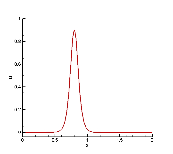
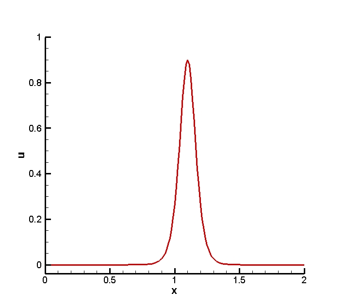
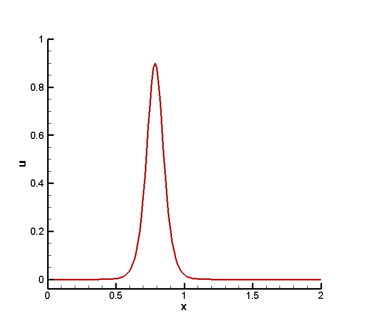
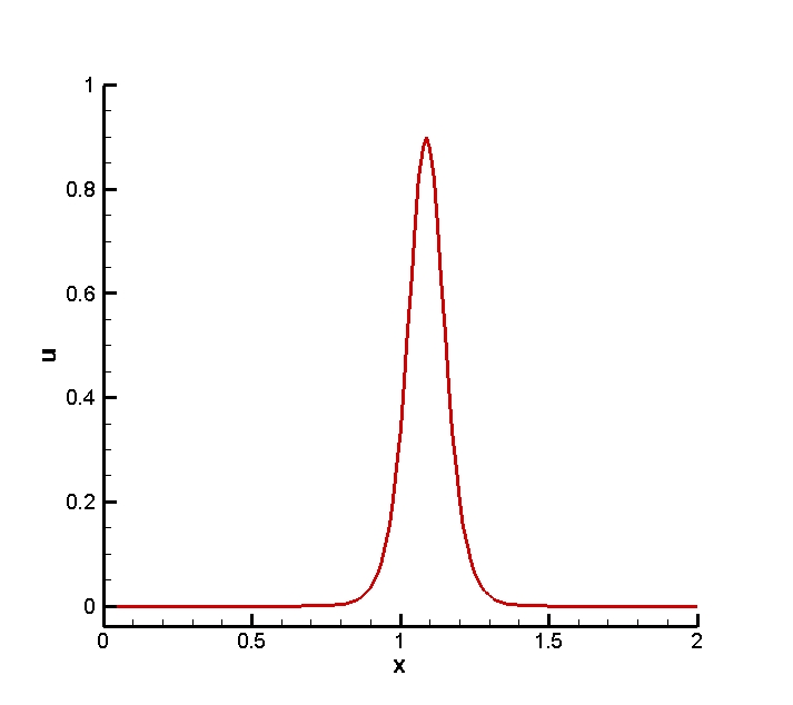
The single soliton case has the initial condition

u​(x,0)=3​c​sech2​(k​(xβˆ’x0))𝑒π‘₯03𝑐superscriptsech2π‘˜π‘₯subscriptπ‘₯0u(x,0)=3c\hbox{sech}^{2}(k(x-x_{0}))

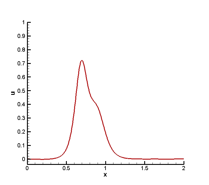
with c=0.3𝑐0.3c=0.3, x0=0.5subscriptπ‘₯00.5x_{0}=0.5, k=12​cΟ΅π‘˜12𝑐italic-Ο΅k=\frac{1}{2}\sqrt{\frac{c}{\epsilon}}, and Ο΅=5Γ—10βˆ’4italic-Ο΅5superscript104\epsilon=5\times 10^{-4}. The solution is computed in x∈(0,2)π‘₯02x\in(0,2) with periodic boundary conditions and shown in Fig.Β 4.1.

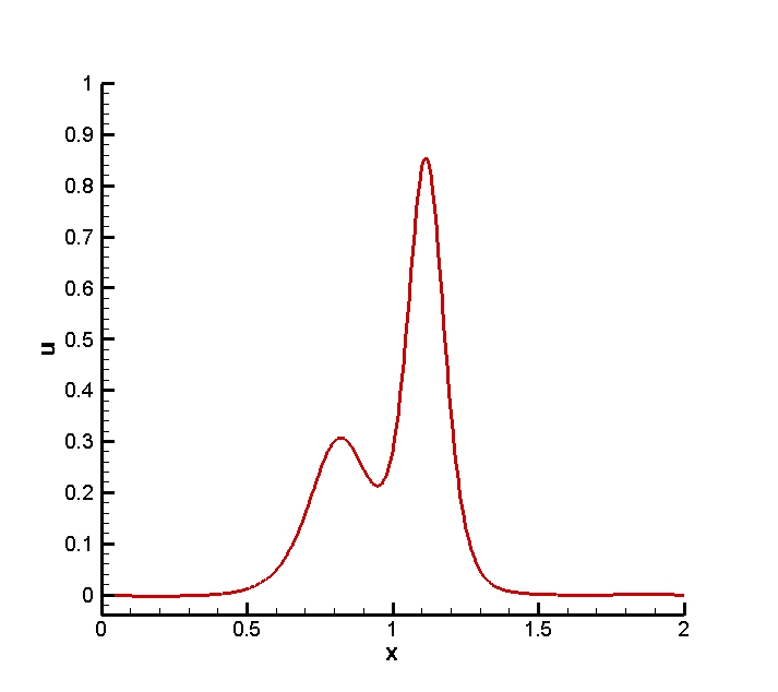
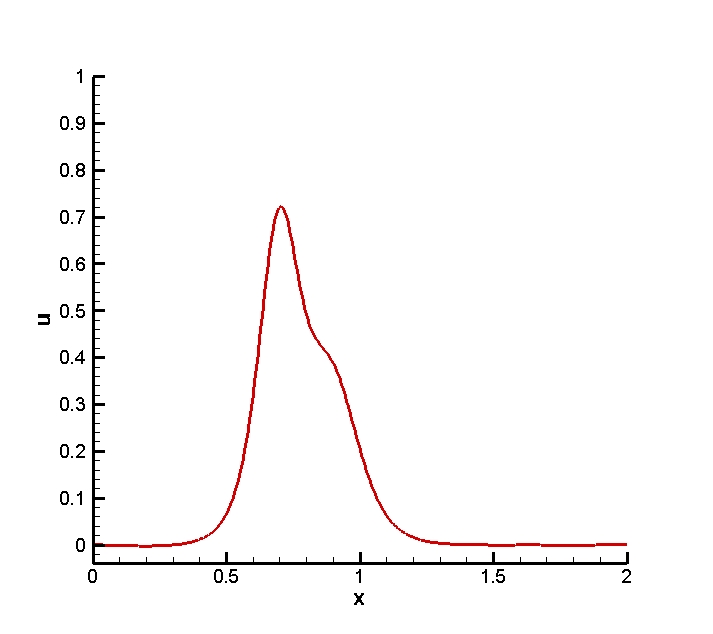
The double soliton collision case has the initial condition

u​(x,0)=3​c1​sech2​(k1​(xβˆ’x1))+3​c2​sech2​(k2​(xβˆ’y))𝑒π‘₯03subscript𝑐1superscriptsech2subscriptπ‘˜1π‘₯subscriptπ‘₯13subscript𝑐2superscriptsech2subscriptπ‘˜2π‘₯𝑦u(x,0)=3c_{1}\hbox{sech}^{2}(k_{1}(x-x_{1}))+3c_{2}\hbox{sech}^{2}(k_{2}(x-y))

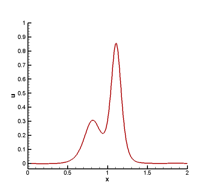
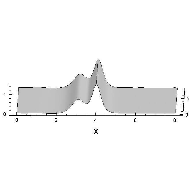
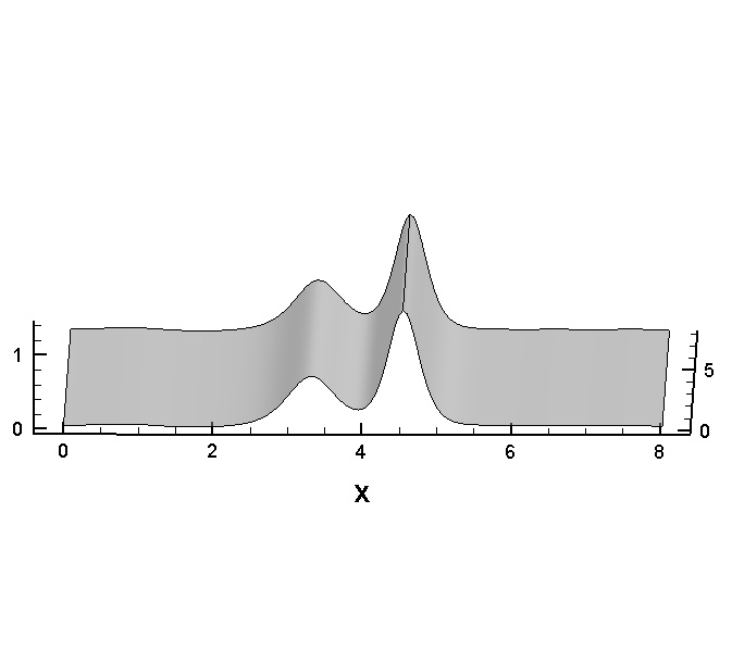
with c1=0.3subscript𝑐10.3c_{1}=0.3, c2=0.1subscript𝑐20.1c_{2}=0.1, x1=0.4subscriptπ‘₯10.4x_{1}=0.4, y=0.8𝑦0.8y=0.8, ki=12​ciΟ΅subscriptπ‘˜π‘–12subscript𝑐𝑖italic-Ο΅k_{i}=\frac{1}{2}\sqrt{\frac{c_{i}}{\epsilon}} for i=1,2𝑖12i=1,2, and Ο΅=4.84Γ—10βˆ’4italic-Ο΅4.84superscript104\epsilon=4.84\times 10^{-4}. The solution shown in Fig.Β 4.2 is computed in x∈(0,2)π‘₯02x\in(0,2) with a periodic boundary condition.
The triple soliton splitting case has the initial condition

u​(x,0)=23​sech2​(xβˆ’1108​ϡ)𝑒π‘₯023superscriptsech2π‘₯1108italic-Ο΅u(x,0)=\frac{2}{3}\hbox{sech}^{2}(\frac{x-1}{\sqrt{108\epsilon}})

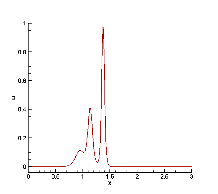
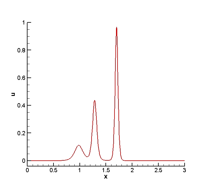
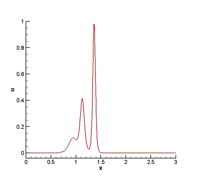
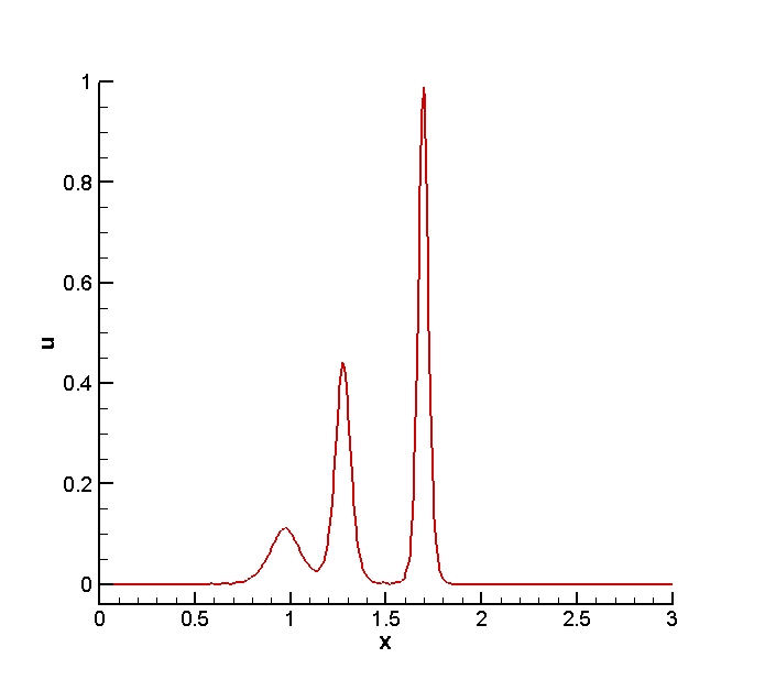
with Ο΅=10βˆ’4italic-Ο΅superscript104\epsilon=10^{-4}. The solution shown in Fig.Β 4.3 is computed in x∈(0,3)π‘₯03x\in(0,3) with a periodic boundary condition.
   

Refer to caption
(a) t=1
Refer to caption
(b) t=2
Refer to caption
(c) t=1
Refer to caption
(d) t=2
Figure 4.1: ExampleΒ 4.3: Single soliton case. Top: P2superscript𝑃2P^{2} elements are used with 160 cells; Bottom: P4superscript𝑃4P^{4} elements are used with 160 cells.


Refer to caption
(a) t=1
Refer to caption
(b) t=2
Refer to caption
(c) t=1
Refer to caption
(d) t=2
Figure 4.2: ExampleΒ 4.3: Double soliton collision case. Top: P2superscript𝑃2P^{2} elements are used with 320 cells; Bottom: P4superscript𝑃4P^{4} elements are used with 320 cells.


Refer to caption
(a) t=1
Refer to caption
(b) t=2
Refer to caption
(c) t=1
Refer to caption
(d) t=2
Figure 4.3: ExampleΒ 4.3: Triple soliton splitting case. Top: P2superscript𝑃2P^{2} elements are used with 320 cells; Bottom: P4superscript𝑃4P^{4} elements are used with 320 cells.
Β Β Β Β Β Β Example 4.4

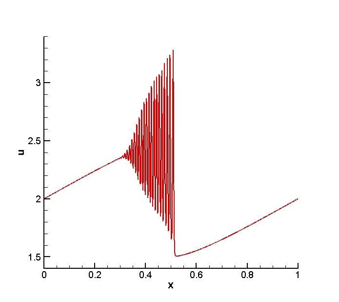
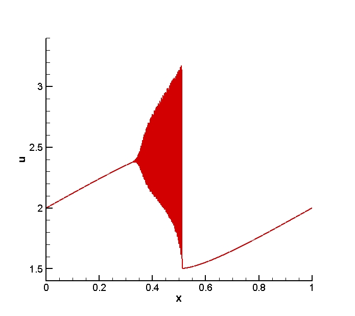
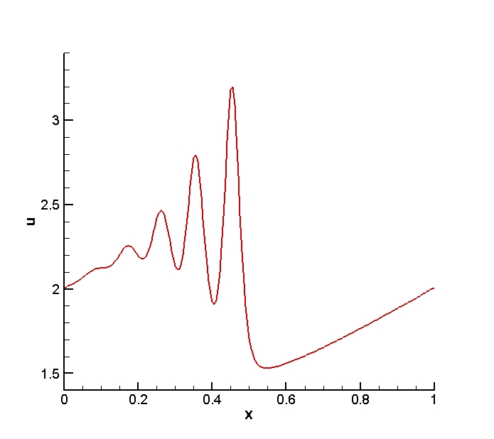
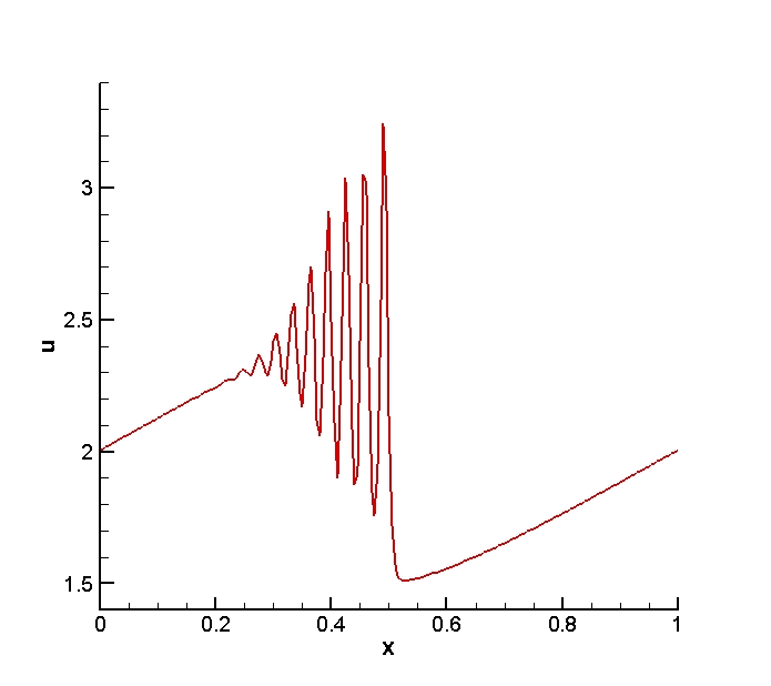
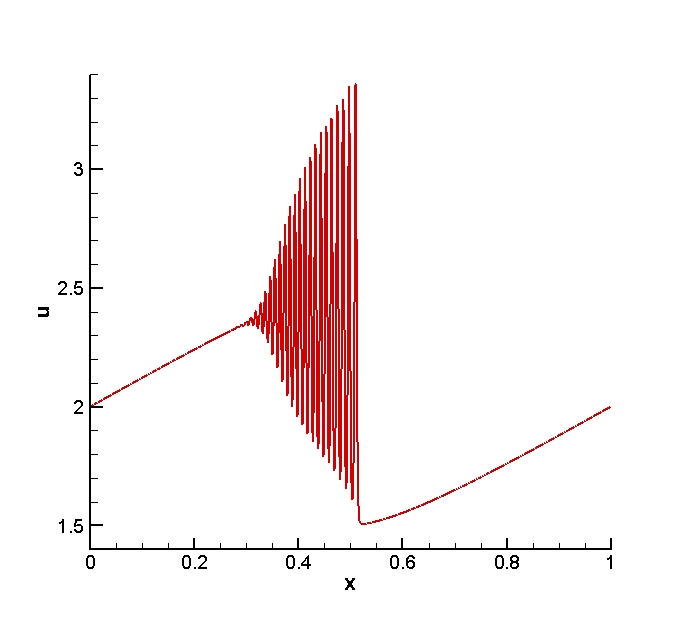
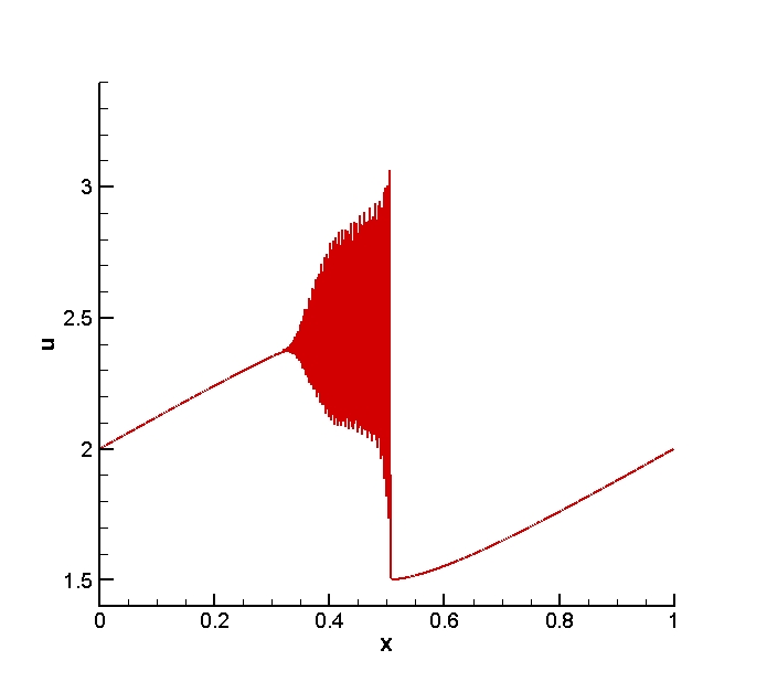
We compute in this example the KdV zero dispersion limit of conservation laws. The equation is

ut+(u22)x+ϡ​ux​x​x=0,x∈(0,1)formulae-sequencesubscript𝑒𝑑subscriptsuperscript𝑒22π‘₯italic-Ο΅subscript𝑒π‘₯π‘₯π‘₯0π‘₯01u_{t}+(\frac{u^{2}}{2})_{x}+\epsilon u_{xxx}=0,\quad x\in(0,1)

subject to the periodic boundary condition and the initial condition

u​(x,0)=2+0.5​sin​(2​π​x).𝑒π‘₯020.5sin2πœ‹π‘₯u(x,0)=2+0.5\hbox{sin}(2\pi x).

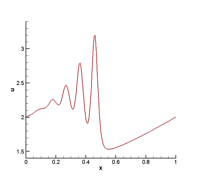
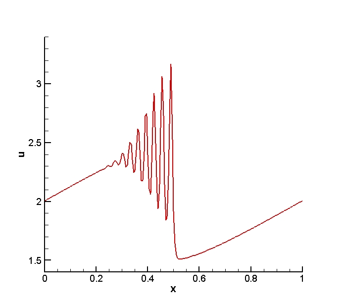
We compute the solution to t=0.5𝑑0.5t=0.5 with Ο΅=10βˆ’4italic-Ο΅superscript104\epsilon=10^{-4}, 10βˆ’5superscript10510^{-5}, 10βˆ’6superscript10610^{-6}, and 10βˆ’7superscript10710^{-7}. These numerical solutions are shown in Figs.Β 4.4 and 4.5.


Refer to caption
(a) Ο΅=10βˆ’4italic-Ο΅superscript104\epsilon=10^{-4}, t=0.5𝑑0.5t=0.5, n=200𝑛200n=200
Refer to caption
(b) Ο΅=10βˆ’5italic-Ο΅superscript105\epsilon=10^{-5}, t=0.5𝑑0.5t=0.5, n=200𝑛200n=200
Refer to caption
(c) Ο΅=10βˆ’6italic-Ο΅superscript106\epsilon=10^{-6}, t=0.5𝑑0.5t=0.5, n=1000𝑛1000n=1000
Refer to caption
(d) Ο΅=10βˆ’7italic-Ο΅superscript107\epsilon=10^{-7}, t=0.5𝑑0.5t=0.5, n=3400𝑛3400n=3400
Figure 4.4: ExampleΒ 4.4: Zero dispersion limit of conservation laws. P2superscript𝑃2P^{2} elements are used.


Refer to caption
(a) Ο΅=10βˆ’4italic-Ο΅superscript104\epsilon=10^{-4}, t=0.5𝑑0.5t=0.5, n=200𝑛200n=200
Refer to caption
(b) Ο΅=10βˆ’5italic-Ο΅superscript105\epsilon=10^{-5}, t=0.5𝑑0.5t=0.5, n=200𝑛200n=200
Refer to caption
(c) Ο΅=10βˆ’6italic-Ο΅superscript106\epsilon=10^{-6}, t=0.5𝑑0.5t=0.5, n=1500𝑛1500n=1500
Refer to caption
(d) Ο΅=10βˆ’7italic-Ο΅superscript107\epsilon=10^{-7}, t=0.5𝑑0.5t=0.5, n=1800𝑛1800n=1800
Figure 4.5: ExampleΒ 4.4: Zero dispersion limit of conservation laws. P4superscript𝑃4P^{4} elements are used.

4.2 Two dimensional examples

Β Β Β Β Β Β Example 4.5

In this example we compute the solution of the linear equation

ut+ux​x​x+uy​y​y=0,(x,y)∈(0,2​π)Γ—(0,2​π)formulae-sequencesubscript𝑒𝑑subscript𝑒π‘₯π‘₯π‘₯subscript𝑒𝑦𝑦𝑦0π‘₯𝑦02πœ‹02πœ‹u_{t}+u_{xxx}+u_{yyy}=0,\quad(x,y)\in(0,2\pi)\times(0,2\pi)

with the initial condition u​(x,y,0)=sin⁑(x+y)𝑒π‘₯𝑦0π‘₯𝑦u(x,y,0)=\sin(x+y) and the periodic boundary condition in both directions. Here, f1​(u)=f2​(u)=0,g12=g21=0,g11​(r)=g22​(r)=r,r1​(u)=r2​(u)=u.formulae-sequencesubscript𝑓1𝑒subscript𝑓2𝑒0subscript𝑔12subscript𝑔210subscript𝑔11π‘Ÿsubscript𝑔22π‘Ÿπ‘Ÿsubscriptπ‘Ÿ1𝑒subscriptπ‘Ÿ2𝑒𝑒f_{1}(u)=f_{2}(u)=0,\quad g_{12}=g_{21}=0,\quad g_{11}(r)=g_{22}(r)=r,\quad r_{1}(u)=r_{2}(u)=u. The exact solution is given by u​(x,y,t)=sin⁑(x+yβˆ’2​t)𝑒π‘₯𝑦𝑑π‘₯𝑦2𝑑u(x,y,t)=\sin(x+y-2t). The L1superscript𝐿1L^{1}, L2superscript𝐿2L^{2}, and L∞superscript𝐿L^{\infty} norm of the error and the convergence order of the scheme are shown in TableΒ 4.3. It can be seen clearly that the scheme with Pksuperscriptπ‘ƒπ‘˜P^{k} elements in DG gives the (k+1)thsuperscriptπ‘˜1th(k+1)^{\text{th}} order of convergence.

Table 4.3: ExampleΒ 4.5: periodic boundary conditions and T=1𝑇1T=1.
kπ‘˜k nΓ—n𝑛𝑛n\times n 10Γ—10101010\times 10 20Γ—20202020\times 20 30Γ—30303030\times 30 40Γ—40404040\times 40 50Γ—50505050\times 50
2 L1superscript𝐿1L^{1} 6.411e-3 4.351e-4 1.058e-4 4.123e-5 2.030e-5
Order 3.88 3.49 3.28 3.18
L2superscript𝐿2L^{2} 6.360e-3 4.563e-4 1.131e-4 4.454e-5 2.207e-6
Order 3.80 3.44 3.24 3.15
L∞subscript𝐿L_{\infty} 7.974e-3 5.973e-4 1.521e-4 6.093e-5 3.041e-5
Order 3.74 3.37 3.18 3.11
3 L1superscript𝐿1L^{1} 5.993e-4 1.537e-5 1.839e-6 4.445e-7 1.571e-7
Order 5.29 5.24 4.94 4.66
L2superscript𝐿2L^{2} 5.923e-4 1.572e-5 1.950e-6 4.821e-7 1.726e-7
Order 5.24 5.15 4.86 4.60
L∞subscript𝐿L_{\infty} 6.745e-4 1.969e-5 2.703e-6 7.006e-7 2.554e-7
Order 5.10 4.90 4.69 4.52
Β Β Β Β Β Β Example 4.6

In this example we consider the Zakharov-Kuznetsov (ZK) equation

ut+u​ux+Ρ​(ux​x​x+uy​y​x)=0.subscript𝑒𝑑𝑒subscript𝑒π‘₯πœ€subscript𝑒π‘₯π‘₯π‘₯subscript𝑒𝑦𝑦π‘₯0\displaystyle u_{t}+uu_{x}+\varepsilon(u_{xxx}+u_{yyx})=0. (4.1)

Here, f1​(u)=u22,f2​(u)=0,g12=g22=0,g11​(r)=g21​(r)=ϡ​r,r1​(u)=r2​(u)=u.formulae-sequenceformulae-sequencesubscript𝑓1𝑒superscript𝑒22formulae-sequencesubscript𝑓2𝑒0subscript𝑔12subscript𝑔220subscript𝑔11π‘Ÿsubscript𝑔21π‘Ÿitalic-Ο΅π‘Ÿsubscriptπ‘Ÿ1𝑒subscriptπ‘Ÿ2𝑒𝑒f_{1}(u)=\frac{u^{2}}{2},\quad f_{2}(u)=0,\quad g_{12}=g_{22}=0,\quad g_{11}(r)=g_{21}(r)=\epsilon r,\quad r_{1}(u)=r_{2}(u)=u. The steady progressive wave solution is of the form

u​(x,y,t)=3​c​sech2​(0.5​cΡ​((xβˆ’c​tβˆ’x0)​cos​θ+(yβˆ’y0)​sin​θ)),𝑒π‘₯𝑦𝑑3𝑐superscriptsech20.5π‘πœ€π‘₯𝑐𝑑subscriptπ‘₯0cosπœƒπ‘¦subscript𝑦0sinπœƒ\displaystyle u(x,y,t)=3c\hbox{sech}^{2}(0.5\sqrt{{\frac{c}{\varepsilon}}}((x-ct-x_{0})\hbox{cos}\theta+(y-y_{0})\hbox{sin}\theta)), (4.2)

where ΞΈπœƒ\theta is an inclined angle with respect to the xπ‘₯x-axis and (x0,y0)subscriptπ‘₯0subscript𝑦0(x_{0},y_{0}) is the location of the peak of the initial u𝑒u. We can see in TablesΒ 4.4 and 4.5 that the method with Pksuperscriptπ‘ƒπ‘˜P^{k} elements gives the (k+1)thsuperscriptπ‘˜1th(k+1)^{\text{th}} order of convergence. The computational domains are (βˆ’16,16)Γ—(βˆ’16,16)16161616(-16,16)\times(-16,16) in Table 4.4 and (0,32)Γ—(0,16)032016(0,32)\times(0,16) in Table 4.5, respectively.

Table 4.4: ExampleΒ 4.6: periodic boundary condition in both directions, c=0.01𝑐0.01c=0.01, Ξ΅=0.01πœ€0.01\varepsilon=0.01, ΞΈ=0πœƒ0\theta=0, x0=0subscriptπ‘₯00x_{0}=0, y0=0subscript𝑦00y_{0}=0, T=1𝑇1T=1.
kπ‘˜k nΓ—n𝑛𝑛n\times n 40Γ—40404040\times 40 50Γ—50505050\times 50 60Γ—60606060\times 60 70Γ—70707070\times 70 80Γ—80808080\times 80
2 L1superscript𝐿1L^{1} 1.515e-6 4.671e-7 2.202e-7 1.120e-7 6.404e-8
Order 5.27 4.12 4.39 4.19
L2superscript𝐿2L^{2} 4.128e-6 1.527e-6 7.131e-7 3.887e-7 2.189e-7
Order 4.46 4.18 3.94 4.30
L∞subscript𝐿L_{\infty} 1.747e-5 7.278e-6 4.573e-6 2.659e-6 1.449e-6
Order 3.92 2.55 3.52 4.55
3 L1superscript𝐿1L^{1} 1.046e-6 2.796e-7 1.249e-7 5.814e-8 2.785e-8
Order 5.91 4.42 4.96 5.51
L2superscript𝐿2L^{2} 2.376e-6 8.512e-7 3.663e-7 1.869e-7 9.563e-8
Order 4.60 4.62 4.37 5.02
L∞subscript𝐿L_{\infty} 8.766e-6 4.474e-6 1.866e-6 1.112e-6 5.968e-7
Order 3.01 4.80 3.36 4.66
Table 4.5: ExampleΒ 4.6: periodic boundary condition in the xπ‘₯x-direction and Dirichlet boundary condition in the y𝑦y-directions, c=0.01𝑐0.01c=0.01, Ξ΅=0.01πœ€0.01\varepsilon=0.01, ΞΈ=Ο€12πœƒπœ‹12\theta=\frac{\pi}{12}, x0=16subscriptπ‘₯016x_{0}=16, y0=8subscript𝑦08y_{0}=8, and T=1𝑇1T=1.
kπ‘˜k nΓ—n𝑛𝑛n\times n 40Γ—40404040\times 40 50Γ—50505050\times 50 60Γ—60606060\times 60 70Γ—70707070\times 70 80Γ—80808080\times 80
2 L1superscript𝐿1L^{1} 1.583e-6 5.111e-7 2.366e-7 1.088e-7 5.919e-8
Order 5.07 4.22 5.04 4.56
L2superscript𝐿2L^{2} 5.009e-6 1.802e-6 8.382e-7 3.922e-7 1.966e-7
Order 4.58 4.20 4.93 5.17
L∞subscript𝐿L_{\infty} 3.623e-5 1.538e-5 6.424e-6 3.400e-6 1.592e-6
Order 3.84 4.79 4.13 5.68
3 L1superscript𝐿1L^{1} 1.523e-6 3.564e-7 1.800e-7 6.543e-8 2.846e-8
Order 6.51 3.75 6.56 6.23
L2superscript𝐿2L^{2} 4.014e-6 1.164e-6 5.582e-7 2.337e-7 1.009e-7
Order 5.55 4.03 5.65 6.29
L∞subscript𝐿L_{\infty} 3.094e-5 9.814e-6 4.009e-6 2.211e-6 8.719e-7
Order 5.15 4.91 3.86 6.97
Β Β Β Β Β Β Example 4.7

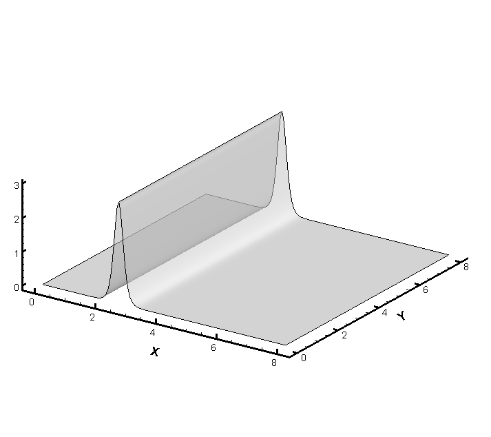
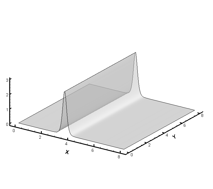
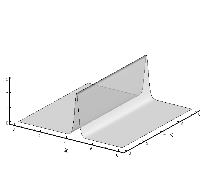
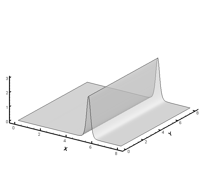
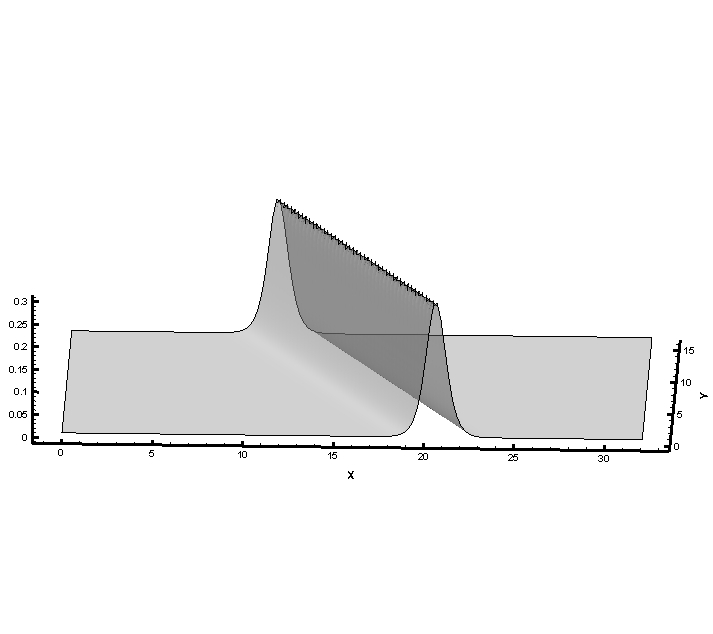
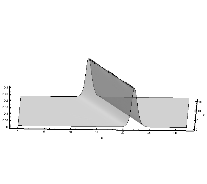
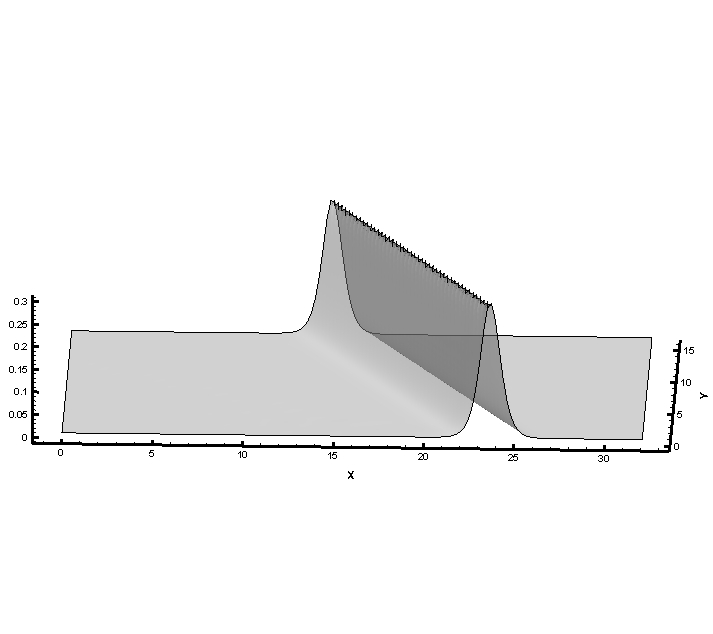
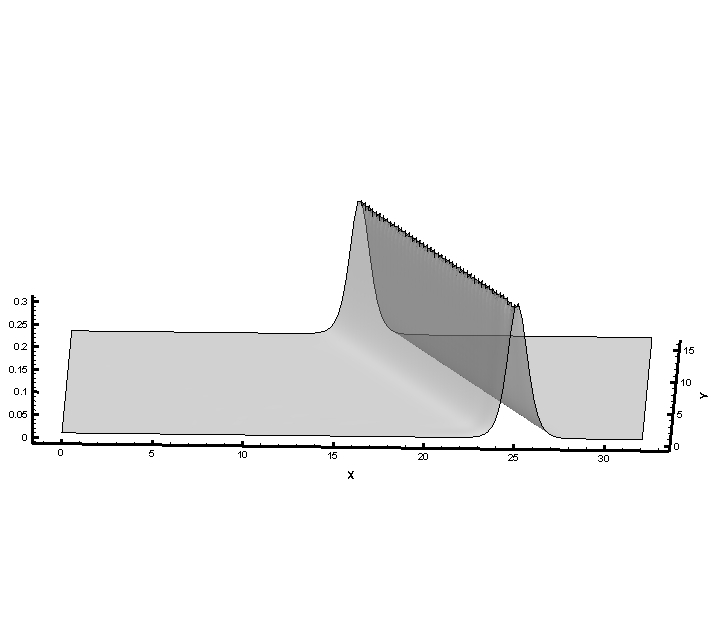
In this example we show the steady progressive wave propagation of the ZK equation (4.1). First, we show the single steady progressive wave in Figs. 4.6 and 4.7 with the initial condition

u​(x,y,0)=3​c​sech2​(0.5​cΡ​((xβˆ’x0)​cos​θ+(yβˆ’y0)​sin​θ)),𝑒π‘₯𝑦03𝑐superscriptsech20.5π‘πœ€π‘₯subscriptπ‘₯0cosπœƒπ‘¦subscript𝑦0sinπœƒ\displaystyle u(x,y,0)=3c\hbox{sech}^{2}(0.5\sqrt{{\frac{c}{\varepsilon}}}((x-x_{0})\hbox{cos}\theta+(y-y_{0})\hbox{sin}\theta)), (4.3)

where ΞΈπœƒ\theta is the inclined angle with respect to the xπ‘₯x-axis. The periodic boundary condition in both xπ‘₯x- and y𝑦y-directions are used when ΞΈ=0πœƒ0\theta=0. Since the solution cannot be periodic in y𝑦y-direction when ΞΈβ‰ 0πœƒ0\theta\neq 0, we use for this case the Dirichlet boundary condition in the y𝑦y-direction and a periodic boundary condition in the xπ‘₯x-direction.

The double soliton collision case has the initial condition

u​(x,y,0)=βˆ‘j=123​cj​sech2​(0.5​cjΡ​((xβˆ’xj)​cos​θ+(yβˆ’yj)​sin​θ)),𝑒π‘₯𝑦0superscriptsubscript𝑗123subscript𝑐𝑗superscriptsech20.5subscriptπ‘π‘—πœ€π‘₯subscriptπ‘₯𝑗cosπœƒπ‘¦subscript𝑦𝑗sinπœƒ\displaystyle u(x,y,0)=\sum\limits_{j=1}^{2}3c_{j}\hbox{sech}^{2}(0.5\sqrt{{\frac{c_{j}}{\varepsilon}}}((x-x_{j})\hbox{cos}\theta+(y-y_{j})\hbox{sin}\theta)), (4.4)

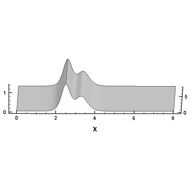
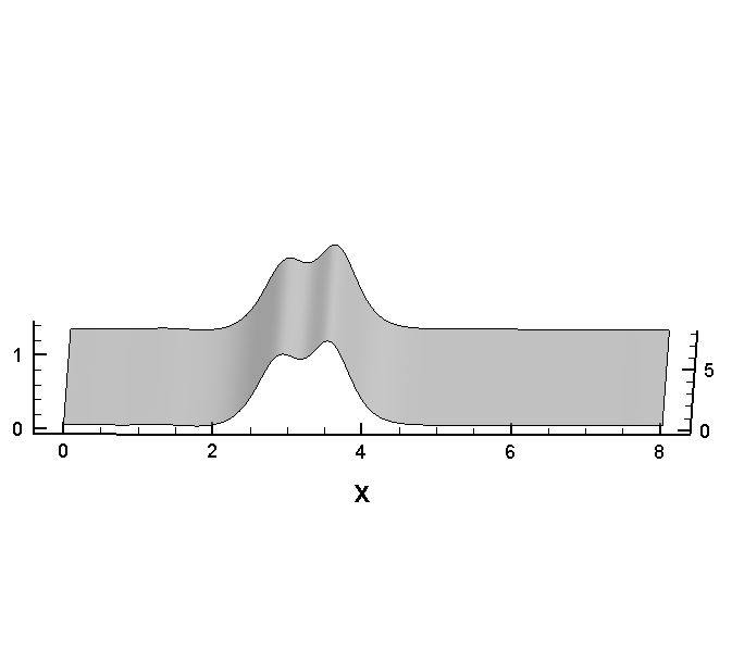
where c1=0.45subscript𝑐10.45c_{1}=0.45, c2=0.25subscript𝑐20.25c_{2}=0.25, Ξ΅=0.01πœ€0.01\varepsilon=0.01, ΞΈ=0πœƒ0\theta=0, x1=2.5subscriptπ‘₯12.5x_{1}=2.5, y1=0subscript𝑦10y_{1}=0, y=3.3𝑦3.3y=3.3, y2=0subscript𝑦20y_{2}=0. The results with periodic boundary conditions in both coordinate directions in (0,8)Γ—(0,8)0808(0,8)\times(0,8) using P2superscript𝑃2P^{2} elements with 150Γ—150150150150\times 150 uniform cells are shown in Fig.Β 4.8.


Refer to caption
(a) t=0𝑑0t=0
Refer to caption
(b) t=1𝑑1t=1
Refer to caption
(c) t=2𝑑2t=2
Refer to caption
(d) t=3𝑑3t=3
Figure 4.6: ExampleΒ 4.7: The single steady progressive wave propagation with the initial condition (4.3). c=1𝑐1c=1, Ξ΅=0.01πœ€0.01\varepsilon=0.01, ΞΈ=0πœƒ0\theta=0, x0=2.5subscriptπ‘₯02.5x_{0}=2.5, y0=4subscript𝑦04y_{0}=4. Periodic boundary condition in both coordinate directions in (0,8)Γ—(0,8)0808(0,8)\times(0,8). P2superscript𝑃2P^{2} elements with 150Γ—150150150150\times 150 uniform cells are used.


Refer to caption
(a) t=0𝑑0t=0
Refer to caption
(b) t=15𝑑15t=15
Refer to caption
(c) t=30𝑑30t=30
Refer to caption
(d) t=45𝑑45t=45
Figure 4.7: ExampleΒ 4.7: The single steady progressive wave propagation with the initial condition (4.3). c=0.1𝑐0.1c=0.1, Ξ΅=0.01πœ€0.01\varepsilon=0.01, ΞΈ=Ο€6πœƒπœ‹6\theta=\frac{\pi}{6}, x0=16subscriptπ‘₯016x_{0}=16, y0=8subscript𝑦08y_{0}=8. Periodic boundary condition in the xπ‘₯x-direction and Dirichlet boundary condition in the y𝑦y-direction in (0,32)Γ—(0,16)032016(0,32)\times(0,16). P2superscript𝑃2P^{2} elements with 150Γ—150150150150\times 150 uniform cells are used.


Refer to caption
(a) t=0𝑑0t=0
Refer to caption
(b) t=1𝑑1t=1
Refer to caption
(c) t=2𝑑2t=2
Refer to caption
(d) t=3𝑑3t=3
Figure 4.8: ExampleΒ 4.7: Double soliton collision profiles and periodic boundary condition in both coordinate directions in (0,8)Γ—(0,8)0808(0,8)\times(0,8). P2superscript𝑃2P^{2} elements with 150Γ—150150150150\times 150 uniform cells are used.
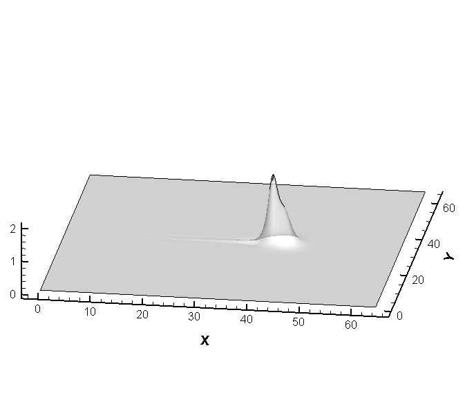
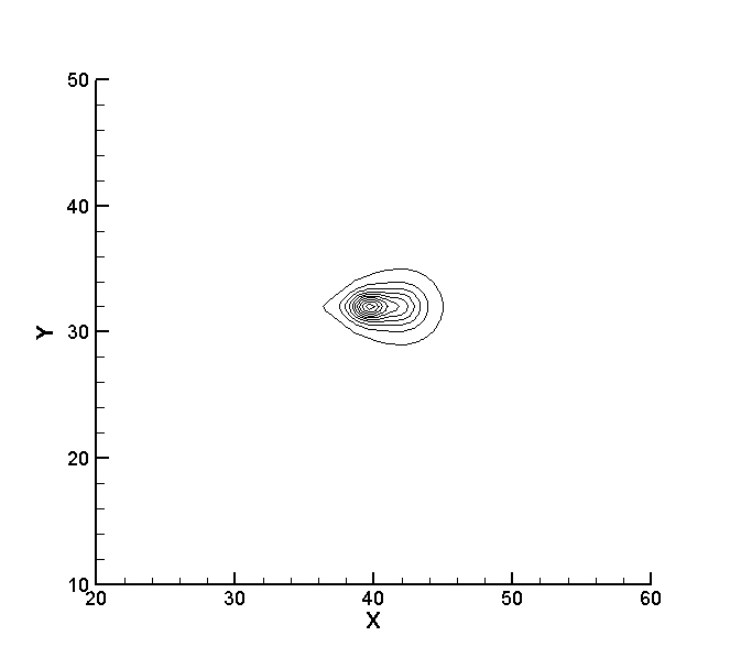
Β Β Β Β Β Β Example 4.8

In this example we show the numerical results for the equation

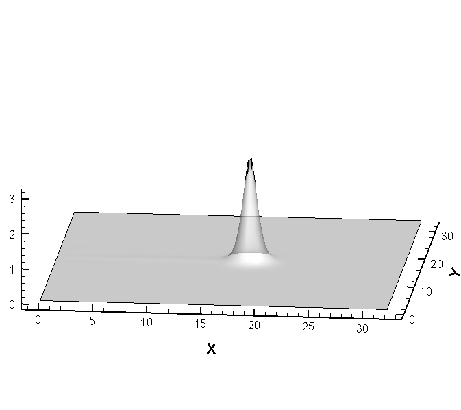
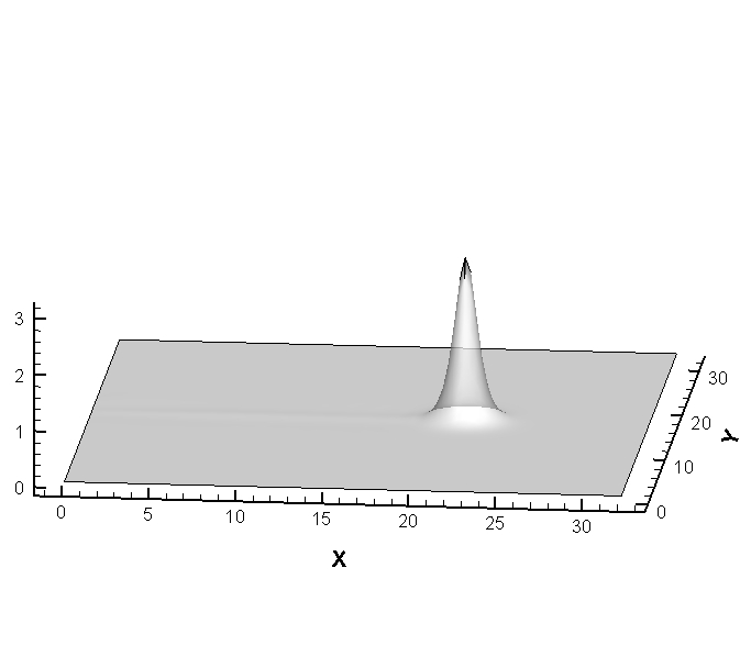
ut+(3​u2)x+ux​x​x+ux​y​y=0.subscript𝑒𝑑subscript3superscript𝑒2π‘₯subscript𝑒π‘₯π‘₯π‘₯subscript𝑒π‘₯𝑦𝑦0\displaystyle u_{t}+(3u^{2})_{x}+u_{xxx}+u_{xyy}=0. (4.5)

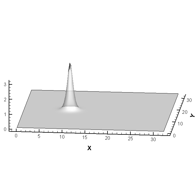
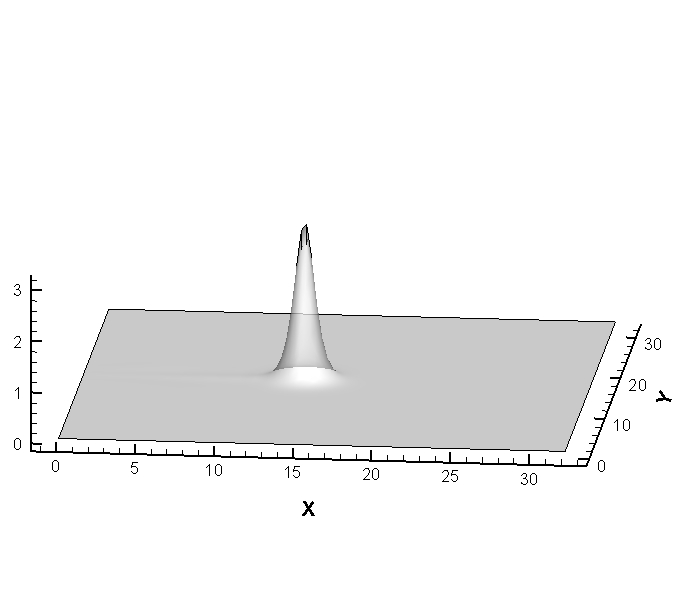
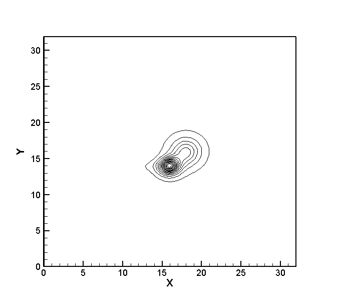
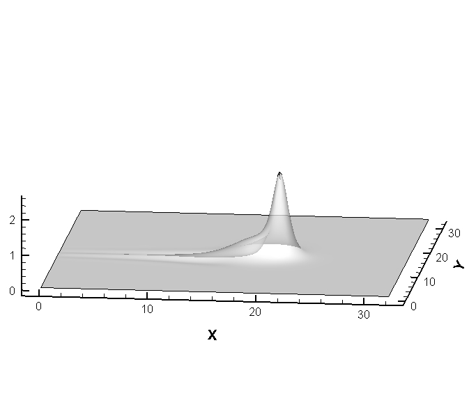
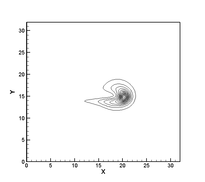
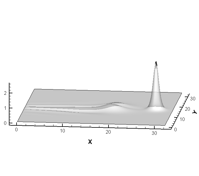
Here, f1​(u)=3​u2,f2​(u)=0,g12=g22=0,g11​(u)=g21​(u)=u,r1​(u)=r2​(u)=u.formulae-sequenceformulae-sequencesubscript𝑓1𝑒3superscript𝑒2formulae-sequencesubscript𝑓2𝑒0subscript𝑔12subscript𝑔220subscript𝑔11𝑒subscript𝑔21𝑒𝑒subscriptπ‘Ÿ1𝑒subscriptπ‘Ÿ2𝑒𝑒f_{1}(u)=3u^{2},\quad f_{2}(u)=0,\quad g_{12}=g_{22}=0,\quad g_{11}(u)=g_{21}(u)=u,\quad r_{1}(u)=r_{2}(u)=u. A cylindrically symmetric solitary solution was obtained and its evolutions as well as interactions were investigated numerically in [10]. This type of solitary solution, also called the bell-shaped pulse, can be expressed as

u​(x,y,t)=c3β€‹βˆ‘n=110a2​n​(cos​(2​n​arccot​(c2​r))βˆ’1),𝑒π‘₯𝑦𝑑𝑐3superscriptsubscript𝑛110subscriptπ‘Ž2𝑛cos2𝑛arccot𝑐2π‘Ÿ1\displaystyle u(x,y,t)=\frac{c}{3}\sum\limits_{n=1}^{10}a_{2n}(\hbox{cos}(2n\,\hbox{arccot}(\frac{\sqrt{c}}{2}r))-1), (4.6)

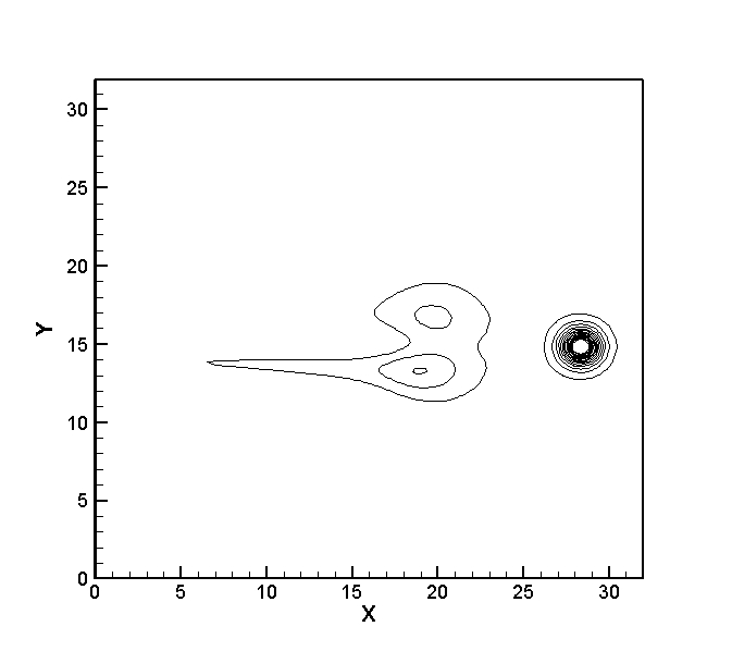
where c𝑐c is the velocity of the solitary wave solution and r=(xβˆ’c​t)2+y2π‘Ÿsuperscriptπ‘₯𝑐𝑑2superscript𝑦2r=\sqrt{(x-ct)^{2}+y^{2}}. The coefficients are collected in TableΒ 4.6 . We use the Dirichlet boundary condition given by the exact solution. The stable propagation of a single pulse is shown in Fig.Β 4.9.

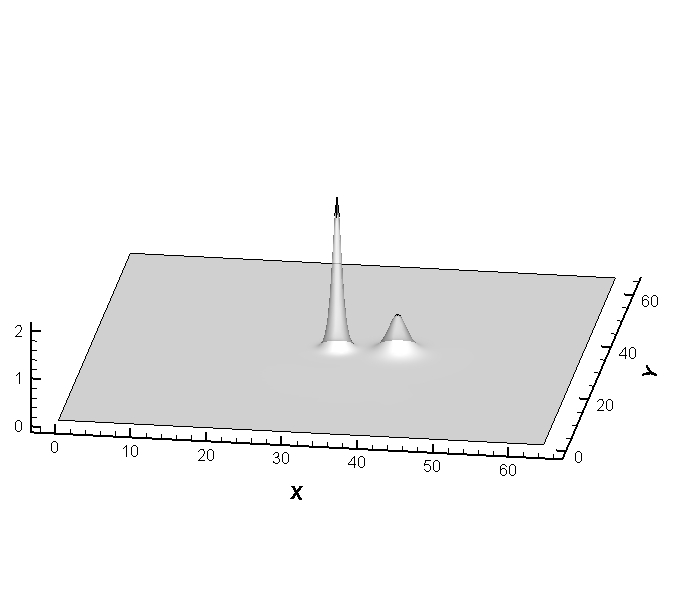
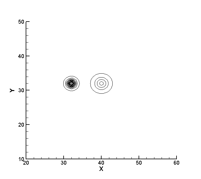
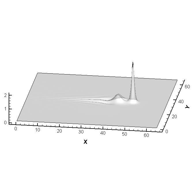
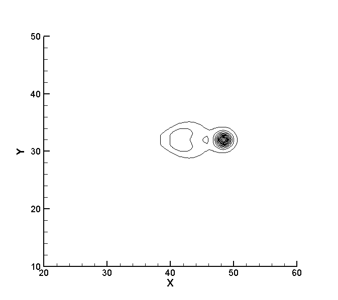
Then, we proceed to show the collision of two pulses with the initial condition

u​(x,y,0)=βˆ‘j=12cj3β€‹βˆ‘n=110a2​n​(cos​(2​n​arccot​(cj2​rj))βˆ’1),𝑒π‘₯𝑦0superscriptsubscript𝑗12subscript𝑐𝑗3superscriptsubscript𝑛110subscriptπ‘Ž2𝑛cos2𝑛arccotsubscript𝑐𝑗2subscriptπ‘Ÿπ‘—1\displaystyle u(x,y,0)=\sum\limits_{j=1}^{2}\frac{c_{j}}{3}\sum\limits_{n=1}^{10}a_{2n}(\hbox{cos}(2n\,\hbox{arccot}(\frac{\sqrt{c_{j}}}{2}r_{j}))-1), (4.7)

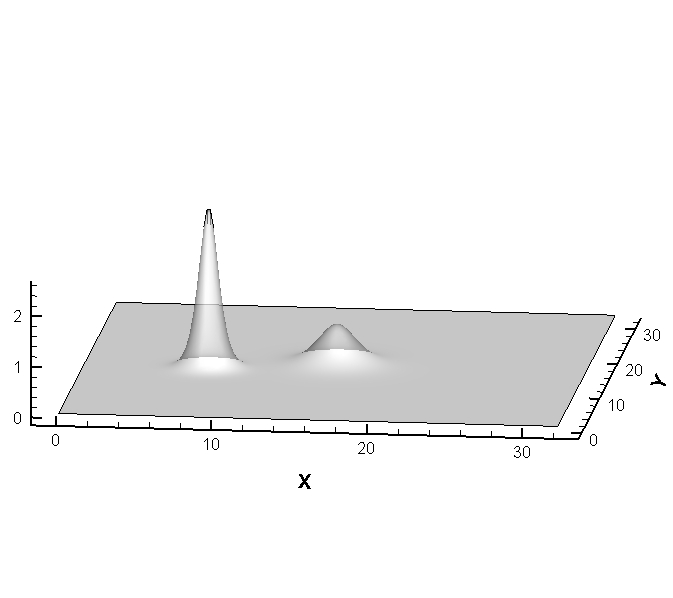
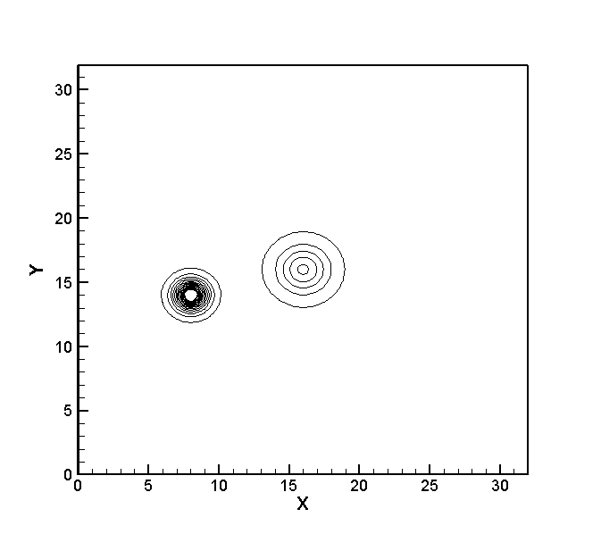
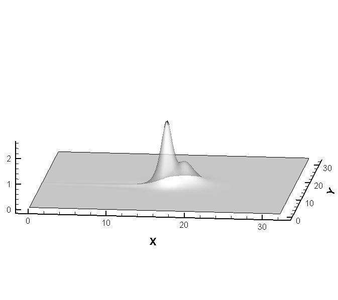
where c1subscript𝑐1c_{1} and c2subscript𝑐2c_{2} are the velocities of the solitary wave solutions, ri=(xβˆ’xi)2+(yβˆ’yi)2subscriptπ‘Ÿπ‘–superscriptπ‘₯subscriptπ‘₯𝑖2superscript𝑦subscript𝑦𝑖2r_{i}=\sqrt{(x-x_{i})^{2}+(y-y_{i})^{2}} (i=1,2)𝑖12(i=1,2), and (xi,yi)subscriptπ‘₯𝑖subscript𝑦𝑖(x_{i},y_{i})’s are the locations of the peaks of u𝑒u. When the centers of the two pulses are situated on the same line with y=const𝑦consty=\text{const}, the collision is called a direct collision and otherwise called a deviated collision [10]. The numerical solutions obtained for the cases of a direct collision and a deviated collision of two pulses are shown in Figs.Β 4.10 and 4.11, respectively.


Refer to caption
(a) t=0𝑑0t=0
Refer to caption
(b) t=1𝑑1t=1
Refer to caption
(c) t=2𝑑2t=2
Refer to caption
(d) t=3𝑑3t=3
Figure 4.9: ExampleΒ 4.8: Evolution of a single bell-shaped pulse solution for (4.5) with c=4𝑐4c=4, x0=10subscriptπ‘₯010x_{0}=10, and y0=16subscript𝑦016y_{0}=16. The used domain is (0,32)Γ—(0,32)032032(0,32)\times(0,32). P2superscript𝑃2P^{2} elements with 100Γ—100100100100\times 100 uniform cells are used.
Table 4.6: ExampleΒ 4.8: Coefficients for the solitary wave solution of the equation (4.5).
n𝑛n a2​nsubscriptπ‘Ž2𝑛a_{2n} n𝑛n a2​nsubscriptπ‘Ž2𝑛a_{2n}
1 -1.25529873 6 -0.00281281
2 0.21722635 7 -0.00138352
3 0.06452543 8 -0.00070289
4 0.00540862 9 -0.00020451
5 -0.00332515 10 -0.00003053


Refer to caption
(a) t=0𝑑0t=0
Refer to caption
(b) t=0𝑑0t=0
Refer to caption
(c) t=2𝑑2t=2
Refer to caption
(d) t=2𝑑2t=2
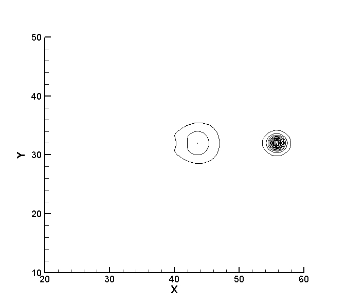
Figure 4.10: ExampleΒ 4.8: Direct collision of two bell-shaped pulses solution for (4.5) with the initial condition (4.7) and c1=4subscript𝑐14c_{1}=4, c2=1subscript𝑐21c_{2}=1, x1=32subscriptπ‘₯132x_{1}=32, y1=32subscript𝑦132y_{1}=32, y=40𝑦40y=40, y2=32subscript𝑦232y_{2}=32, and Dirichlet boundary condition. The computational domain is (0,64)Γ—(0,64)064064(0,64)\times(0,64). P2superscript𝑃2P^{2} elements with 200Γ—200200200200\times 200 uniform cells are used.

%Ν¬ ΝΌ ΔΌ    

Refer to caption
(e) t=4𝑑4t=4
Refer to caption
(f) t=4𝑑4t=4
Refer to caption
(g) t=6𝑑6t=6
Refer to caption
(h) t=6𝑑6t=6
Figure 4.10: (continued)


Refer to caption
(a) t=0𝑑0t=0
Refer to caption
(b) t=0𝑑0t=0
Refer to caption
(c) t=2𝑑2t=2
Refer to caption
(d) t=2𝑑2t=2
Figure 4.11: ExampleΒ 4.8: Deviated collision of two bell-shaped pulses solution for (4.5) with the initial condition (4.7) and c1=4subscript𝑐14c_{1}=4, c2=1subscript𝑐21c_{2}=1, x1=8subscriptπ‘₯18x_{1}=8, y1=14subscript𝑦114y_{1}=14, y=16𝑦16y=16, y2=16subscript𝑦216y_{2}=16. and Dirichlet boundary condition. The computational domain is (0,32)Γ—(0,32)032032(0,32)\times(0,32). P2superscript𝑃2P^{2} elements with 150Γ—150150150150\times 150 uniform cells are used.

%Ν¬ ΝΌ ΔΌ


Refer to caption
(e) t=3𝑑3t=3
Refer to caption
(f) t=3𝑑3t=3
Refer to caption
(g) t=5𝑑5t=5
Refer to caption
(h) t=5𝑑5t=5
Figure 4.11: (continued)

5 Conclusions

In the previous sections we have studied a hybrid LDG-HWENO scheme for solving KdV-type equations. The scheme uses the cell averages of the physical solution and first moment(s) as unknown variables (a feature of HWENO) while approximates high order spatial derivatives using the local DG method. It has less unknown variables than a pure LDG method and can be applied to problems involving high order spatial derivatives. Numerical results have been presented for a selection of one and two dimensional linear and nonlinear examples. They confirm the designed convergence order of the scheme.

The new scheme employs an explicit TVD Runge-Kutta method for time integration and is subject to the CFL condition which requires an extremely small time step restriction of the form Δ​t≀C​Δ​x3Δ𝑑𝐢Δsuperscriptπ‘₯3\Delta t\leq C\Delta x^{3}. How to avoid this restriction using suitable implicit time discretization will be the subject of future work.

References

  • [1] D. S. Balsara, C. Altmann, C.-D. Munz, M. Dumbser, A sub-cell based indicator for troubled zones in RKDG schemes and a novel class of hybrid RKDG+HWENO shemes, J. Comput. Phys., 226 (2007), 586-620.
  • [2] B. Cockburn, C.-W. Shu, TVB Runge-Kutta local projection discontinuous Galerkin finite element method for scalar conservation laws II: General framework, Math. Comp., 52 (1989), 411-435.
  • [3] B. Cockburn, S.-Y. Lin, C.-W. Shu, TVB Runge-Kutta local projection discontinuous Galerkin finite element method for scalar conservation laws III: One dimensional systems, J. Comput. Phys., 84 (1989), 90-113.
  • [4] B. Cockburn, S. Hou, C.-W. Shu, TVB Runge-Kutta local projection discontinuous Galerkin finite element method for scalar conservation laws IV: The multidimensional case, Math. Comp., 54 (1990), 545-581.
  • [5] B. Cockburn, C.-W. Shu, TVB Runge-Kutta local projection discontinuous Galerkin finite element method for scalar conservation laws V: Multidimensional systems, J. Comput. Phys., 141 (1998), 199-224.
  • [6] B. Cockburn, C.-W. Shu, The local discontinuous Galerkin method for time-dependent convection-diffusion systems, SIAM J. Numer. Anal., 35 (1998), 2440-2463.
  • [7] M. Dumbser, Arbitrary high order PNPM schemes on unstructured meshes for the compressible Navier-Stokes equations, Computers & Fluids, 39 (2010), 60-76.
  • [8] M. Dumbser, D. S. Balsara, E. F. Toro and C. D. Munz, A unified framework for the construction of one-step finite volume and discontinuous Galerkin schemes on unstructured meshes, J. Comput. Phys., 227 (2008), 8209-8253.
  • [9] B.-F. Feng, T. Kawahara, T. Mitsui, A conservative spectral method for several two-dimensional nonlinear wave equations, J. Comput. Phys., 153(1999), 467-487.
  • [10] H. Iwasaki, S. Toh, T. Kawahara, Cylindrical quasi-solitons of the Zakharov-Kuznetsov equation, Physica D,43(1990), 293-303.
  • [11] G. Jiang, C.-W. Shu, Efficient implementation of weighted ENO schemes, J. Comput. Phys., 126 (1996), 202-228.
  • [12] G. Jiang, C.-W. Shu, On cell entropy inequality for discontinuous Galerkin methods, Math. Comp., 62 (1994), 531-538.
  • [13] D. Korteweg, G. Varies, On the change of form of long waves advancing in a rectangular canal and on a new type of long stationary waves, Philos. Mag., 39 (1895), 422-443.
  • [14] X. Liu, S. Osher, T. Chan, Weighted essentially non-oscillatory schemes, J. Comput. Phys., 115 (1994), 200-212.
  • [15] H. Luo, L. Luo, R. Nourgaliev, V. A. Mousseau and N. Dinh, A reconstructed discontinuous Galerkin method for the compressible Navier-Stokes equations on arbitrary grids, J. Comput. Phys., 229 (2010), 6961-6978.
  • [16] H. Nishiyama, T. Noi, S. Oharu, Conservative finite difference schemes for the generalized Zakharov-Kuznetsov equations, J. Comput. Appl. Math., 236 (2012), 2998-3006.
  • [17] J. Qiu, C.-W. Shu, Hermite WENO schemes and their application as limiters for Runge-Kutta discontinuous Galerkin method: one-dimensional case, J. Comput. Phys., 193 (2003), 115-135.
  • [18] J. Qiu, C.-W. Shu, Hermite WENO schemes and their application as limiters for Runge-Kutta discontinuous Galerkin method II: two dimensional case, Computers & Fluids, 34 (2005), 642-663.
  • [19] W. H. Reed, T. R. Hill, Triangular mesh methods for neutron transport equation, Los Alamos Scientific Laboratory Report LA-UR-73-479 (1973).
  • [20] J. Shi, C. Hu, C.-W. Shu, A technique of treating negative weights in WENO schemes, J. Comput. Phys., 175 (2002), 108-127.
  • [21] C.-W. Shu, Total-variation-diminishing time discretizations, SIAM J. Sci. Stat. Comput., 9 (1988), 1073-1084.
  • [22] C.-W. Shu, S. Osher, Efficient implementation of essentially non-oscillatory shock-capturing schemes, J. Comput. Phys. 77 (1988), 439-471.
  • [23] C.-W. Shu, S. Osher, Efficient implementation of essentially non-oscillatory shock-capturing schemes, II, J. Comput. Phys. 83 (1989), 32-78.
  • [24] Y. Xia, Y. Xu, C.-W. Shu, Efficient time discretization for local discontinuous Galerkin methods, Discrete Contin. Dyn. Syst. Ser. B, 8 (2007), 677-693.
  • [25] Y. Xu, C.-W. Shu, Local discontinuous Galerkin methods for high-order time-dependent partial differential equations, Commun. Comput. Phys., 7 (2010), 1-46.
  • [26] Y. Xu, C.-W. Shu, Local discontinuous Galerkin methods for two classes of two-dimensional nonlinear wave equations, Physica D, 208 (2005), 21-58.
  • [27] J. Yan, C.-W. Shu, A local discontinuous Galerkin method for KdV type equations, SIAM J. Numer. Anal., 40 (2002), 769-791.
  • [28] F. Zheng and J. Qiu, Directly solving the Hamilton-Jacobi equations by Hermite WENO Schemes, submitted to J. Comput. Phys..