The star cluster mass–galactocentric radius relation: Implications for cluster formation

Abstract

Whether or not the initial star cluster mass function is established through a universal, galactocentric-distance-independent stochastic process, on the scales of individual galaxies, remains an unsolved problem. This debate has recently gained new impetus through the publication of a study that concluded that the maximum cluster mass in a given population is not solely determined by size-of-sample effects. Here, we revisit the evidence in favor and against stochastic cluster formation by examining the young ($\lesssim$ a few $\times 10^{8}$ yr-old) star cluster mass–galactocentric radius relation in M33, M51, M83, and the Large Magellanic Cloud. To eliminate size-of-sample effects, we first adopt radial bin sizes containing constant numbers of clusters, which we use to quantify the radial distribution of the first- to fifth-ranked most massive clusters using ordinary least-squares fitting. We supplement this analysis with an application of quantile regression, a binless approach to rank-based regression taking an absolute-value-distance penalty. Both methods yield, within the $1\sigma$ to $3\sigma$ uncertainties, near-zero slopes in the diagnostic plane, largely irrespective of the maximum age or minimum mass imposed on our sample selection, or of the radial bin size adopted. We conclude that, at least in our four well-studied sample galaxies, star cluster formation does not necessarily require an environment-dependent cluster formation scenario, which thus supports the notion of stochastic star cluster formation as the dominant star cluster-formation process within a given galaxy.

1 Introduction

Although the initial cluster mass function (ICMF) appears to be universal (de Grijs et al., 2003; Portegies Zwart et al., 2010; Fall & Chandar, 2012), the formation conditions of the highest-mass clusters are still subject to significant debate. Proponents of one school of thought suggest that the formation of the most massive clusters in a given volume or during a specific time period is independent of environment (Gieles et al., 2006; Gieles, 2009) and, consequently, that the “size-of-sample” effect determines the masses of the most massive clusters in a given cluster population (e.g., Hunter et al. 2003). Alternatively, the formation of the most massive clusters may require special physical conditions, such as high ambient pressure or enhanced gas densities, which might indeed be environment-dependent. In the context of the ICMF, its possible environmental dependence within a given galaxy could be demonstrated through careful analysis of its relation to galactocentric distance, i.e., by assessment of the “star cluster mass–galactocentric radius relation.” Larsen (2009) modeled the ICMFs in actively star-forming spiral and starburst galaxies, adopting a single Schechter function, and found that the ICMF’s chracteristic cut-off mass at the high-mass end is higher for starburst galaxies than for more quiescent spiral galaxies resembling the Milky Way. This suggests that this global difference may be owing to the high-pressure environments in starburst galaxies.

Pflamm-Altenburg et al. (2013; henceforth PA13) explored the apparent cluster mass–galactocentric radius relationship of young star clusters in Messier 33 (M33, the Triangulum galaxy) based on the data set of Sharma et al. (2011). They claimed to have ruled out the size-of-sample effect as a mechanism driving massive cluster formation and concluded that very massive star clusters may indeed require special physical conditions to form, and thus that the formation of young star clusters is not a stochastic process. PA13’s claims appear strong, in the sense that they purport to expose deficiencies apparently perpetrated by the authors of a number of previous analyses (see also Cameron 2013). However, the scientific strategy employed in these previous studies appears entirely reasonable: namely, their authors compare observational data against a null distribution model and, in the event of observing a reasonable agreement, they decided not to reject the null. Indeed, the quote from past research highlighted by PA13 shows that the earlier researchers were careful to avoid the common logical fallacy of treating non-rejection as support for the null: “Our conclusion [in support of the random drawing hypothesis] remains provisional” (the text within square brackets is ours). Unfortunately, however, the data set used by PA13 is not suitable for the purposes of their analysis (for evidence, see Section 2.1). The validity of their conclusions must thus be revisited.

In this paper, we use observations of young clusters in both Messier 51 (M51, the Whirlpool galaxy) and Messier 83 (M83) to independently test PA13’s conclusions. We do not only use the ordinary least-squares (OLS) method employed by these latter authors, but we also introduce “quantile regression” (QR) as a more suitable and highly robust statistical approach to support our conclusions. We focus predominantly on the results for M51, since they are the strongest. In Section 2, we explain why we discard all currently available cluster data sets pertaining to $\lesssim 10$ Myr-old clusters in M33 (which corresponds to the age range selected by PA13) and select the cluster samples in M51 and M83 instead (but see Section 7 for a brief revisit of the M33 cluster population). We also apply our analysis approach to the lower-mass cluster sample in the Large Magellanic Cloud (LMC). In Section 4, we apply both methods to M51 and show that any radial dependence is rather weak, a statement for which we present statistically robust evidence. In Section 5, we discuss the dependence of our results on our adoption of the maximum cluster age, minimum cluster mass, and bin size. We conclude that variation of the lower-mass limit has a significant impact on the results, whereas varying the applicable age range is less important. We follow up this analysis with similar analyses applied to the M83 as well as to the LMC and M33 cluster populations in Sections 6 and 7, respectively. In Section 8, we briefly summarize the paper and restate our main conclusions.

2 Observational Datasets

Our analysis relies on having access to statistically significant numbers of young clusters with reliable age and mass estimates. In addition, we require the host galaxies to exhibit a reasonable symmetry so that radial averaging can be performed appropriately. In the local Universe, the most suitable star cluster samples that are readily available for our purpose include those hosted by M33, M51, and M83, as well as the LMC cluster population (although the latter galaxy is not as symmetrical as its larger spiral counterparts).

2.1 The M33 Cluster Population

PA13 based their results for M33 on the $24\mu$m-selected data set of Sharma et al. (2011). Therefore, as a first step, we attempted to retrieve this database ourselves in order to check their results. However, we soon learned that Sharma et al. (2011)’s “cleaned” dataset of 648 objects has not been made publicly available, since it consists of an inhomogeneous mixture of object types, including genuine young clusters, but also Hii regions and unidentified asymptotic giant branch stars. Nevertheless, and despite these concerns (voiced by the original authors themselves), Sharma et al. (2011) proceeded to apply statistical analysis tools to both their original, highly contaminated sample of 915 sources and the cleaned data set, referring to the latter as the “young star cluster sample.” Upon contacting these authors, we learned that the individual cluster ages and masses would be insufficiently accurate for the type of analysis we intended to embark on (S. Sharma 2014, private communication). They recommended us not to use their data for exploration of the cluster mass–galactocentric radius relation, given that they were well aware of significant, persistent contamination of even their cleaned data set by spurious, non-cluster objects. However, these concerns were not well communicated in their peer-reviewed article, which led PA13 to chase after what transpired to be a poorly defined, inhomogeneous dataset.

We therefore explored alternative databases containing cluster age and mass estimates for significant samples of M33 clusters. A subset of the current authors published the current most up-to-date and most carefully defined M33 cluster data set (Fan & de Grijs, 2014). The latter sample of star clusters was mainly selected from San Roman et al. (2010), whose database is, in turn, based on observations with the MegaCam camera mounted on the Canada–France–Hawai’i Telescope. Fan & de Grijs (2014) derived photometric and physical parameters for 588 clusters and cluster candidates from archival $UBVRI$ images from the Local Group Galaxies Survey. Supplemented by 120 confirmed star clusters from the updated, 2010 version of Sarajedini & Mancone (2007), the total number of clusters in their sample reached 708. However, although 69% of these clusters and cluster candidates are characterized by ages younger than 2 Gyr, few young clusters with ages of $\lesssim 10^{7}$ yr are included in the final database. This limitation implies that this database cannot be used either to conclusively examine the formation modes of young star clusters following PA13. We are not aware of any other M33 cluster database that could currently serve this purpose.

2.2 M51 and M83 Cluster Data

The M51 dataset used in this paper, which contains many young star clusters, was published by Chandar et al. (2011). These authors made use of multi-color F435W (“$B$”), F555W (“$V$”), F814W (“$I$”) and F658N (“$\text{H}\alpha$”) images of M51 obtained with the Hubble Space Telescope’s (HST) Advanced Camera for Surveys, combined with F336W (“$U$”) pointings obtained with the HST’s Wide-Field and Planetary Camera-2. They estimated the age and extinction pertaining to each cluster by performing a minimum-$\chi^{2}$ fit, comparing the measurements in five filters ($UBVI$, $\text{H}\alpha$) with predictions from the Bruzual & Charlot (2003) simple stellar population (SSP) models. They assumed solar metallicity, $Z=0.02$ (which is appropriate for young clusters in M51; Moustakas et al. 2010), a Salpeter (1955) stellar initial mass function (IMF), and a Galactic-type extinction law. They constructed the mass function (MF) of 3812 intermediate-age, (1–4)$\times 10^{8}$ yr-old star clusters in a $3\times 7$ kpc² region of M51. For reasons of consistency and comparison with previous work, here we adopt Chandar et al.’s (2011) $\sim 90$% completeness limit of $\sim 6000M_{\odot}$ (but see Section 5.2 for a detailed analysis).

For M83, we adopted the dataset taken from Bastian et al. (2011). These authors used Early Release Science data of two adjacent fields in M83, observed with the HST/Wide Field Camera-3. The data pertaining to the inner field were presented by Chandar et al. (2010). The latter authors made use of observations in the F336W ($U$), F438W ($B$), F555W ($V$), F657N (H$\alpha$), and F814W ($I$) filters. The outer-field data were imaged in the same filters. Bastian et al. (2011) estimated the age, mass, and extinction affecting each of their M83 sample clusters by comparing the observed cluster magnitudes with SSP models. They compared the results from their application of two methods, including those returned by the 3DEF fitting code (Bastian et al., 2005) combined with the galev SSP models, as well as results obtained with the fitting procedure of Adamo et al. (2010a, b) and the yggdrasil SSP models (Zackrisson et al., 2011). Bastian et al. (2011) adopted a metallicity of $2.5Z_{\odot}$ and a Kroupa-type stellar IMF. Both sets of models also include contributions from nebular emission, which is helpful in distinguishing old clusters from young, highly extinguished clusters (Chandar et al., 2010; Konstantopoulos et al., 2010) and contributes to the broad-band colors, sometimes significantly so (Anders & Fritze-v. Alvensleben 2003). Both methods yielded consistent ages and masses for the clusters. In the present paper, we have adopted the ages and masses for 940 star clusters and cluster candidates in M83 derived using the Adamo et al. (2010a) method.

2.3 Star Clusters in the LMC

The statistically complete LMC cluster database we adopted was published by Baumgardt et al. (2013). These authors used four recent compilations of LMC star cluster parameters to derive a combined catalog of LMC clusters. Their primary data set is that of Glatt et al. (2010), who used data from the Magellanic Clouds Photometric Surveys (Zaritsky et al., 2002, 2004), combined with isochrone fitting, to derive ages and luminosities for 1193 populous star clusters in a 64 deg² area of the LMC. Their second data set is the catalog of Pietrzyński & Udalski (2000), who used $BVI$ data from the Optical Gravitational Lensing Experiment II (ogle ii) (Udalski et al., 1998), again combined with isochrone fitting to derive ages of approximately 600 star clusters located in the central parts of the LMC, with ages younger than 1.2 Gyr. Baumgardt et al. (2013) also include cluster ages from both Milone et al. (2009) and Mackey & Gilmore (2003). Many of the ages in these catalogs were derived on the basis of HST data.

3 Importance of a “truncation mass”

Numerous previous ICMF determinations have also found power-law functions with indices close to $-2$ (e.g., Zhang & Fall 1999; de Grijs et al. 2003; Bik et al. 2003; McCrady & Graham 2007; among many others). In addition, there is mounting evidence of the reality of a “truncation mass” in cluster MFs which varies among galaxies (e.g., Gieles et al. 2006; Bastian 2008; Larsen 2009; Maschberger & Kroupa 2009; Bastian et al. 2012; Kostantopolous et al. 2013; Adamo & Bastian 2015). Indeed, the functional form of the ICMF for young star clusters is well represented by a Schechter (1976) distribution,

$$\psi(M)=\frac{\textrm{d}N}{\textrm{d}M}=AM^{-\beta}\exp(-M/M_{\star}),$$

where $M_{\star}$ is the truncation mass. Gieles et al. (2006) and Gieles (2009) reported a truncation mass that is different for spiral and starburst galaxies. For Milky Way-type spiral galaxies, $M_{\star}\approx 2\times 10^{5}M_{\odot}$ (Gieles et al. 2006; Larsen 2009). For interacting galaxies and luminous infrared galaxies, Bastian (2008) obtained $M_{\star}\geq 10^{6}M_{\odot}$. In the present paper, we focus on the importance of a possible environmental influence at different galactocentric radii in the same galaxy. In this context, different truncation masses in different galaxy types do not rule out stochastic cluster formation in a given galaxy.

In previous research on the reality of truncation masses, the age of the cluster samples used for the analyses usually extended to a few $\times 10^{8}$ yr. Whether the high-mass end of the cluster MF is affected by a truncation cannot always be confirmed convincingly because of the often small numbers of young clusters available. We can gain statistical insights based on Chandar et al.’s (2010) M51 dataset by conducting a Monte Carlo test to check for the existence, if any, of a truncation mass in the clusters’ MF (e.g., Bastian et al. 2012). We derive $M_{\star}\approx 10^{5}M_{\odot}$, with $\beta\sim 2$, both for cluster ages younger than $10^{7}$ yr and for ages up to $10^{8}$ yr: see Fig. 1 and 1, respectively. To our knowledge, this is the first confirmation of a truncation mass for such young clusters in a spiral galaxy. We note that Chandar et al. (2011) did not find any evidence for curvature in the MF of their M51 cluster sample. We cannot directly compare our results with theirs, however, since Chandar et al. (2011) analyzed the MF for clusters with ages in the range of $(1-4)\times 10^{8}$ yr, which is significantly older than the young age range considered here. Those authors comment on the need to consider the effects of cluster disruption, for which they quote a typical timescale of $2\times 10^{8}$ yr for $10^{4}M_{\odot}$ clusters. Asuming “standard” disruption analysis (see Chandar et al. 2011), our young sample is expected to be negligibly affected by such effects.

We note that the fit result strongly depends on the lower mass limit adopted. The lower mass limit is mainly affected by the level of the sample’s incompleteness. In turn, this dependence can be used, in fact, to determine the statistically meaningful sampling limit to the low-mass end of randomly sampled clusters. For a minumum mass of $10^{3}M_{\odot}$ (following PA13), the dataset is poorly described by either a pure power-law or a Schechter MF (see Fig. 1). The best fit is obtained for a lower mass limit of approximately 5000–7000 $M_{\odot}$. As we will show in Section 5.2, our simulations based on mock cluster populations imply that a completeness level $\gtrsim 80$% would be suitable to construct cumulative MFs. We will also show that the M51 cluster sample is best characterized using a completeness limit in the range from $\sim 3500M_{\odot}$ to $5000M_{\odot}$.

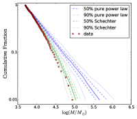
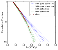
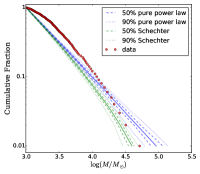
Figure 1: Cumulative cluster mass fractions for M51. Red dots: Observational data. Green line: Schechter function. Blue line: pure power law. (a) Age $<10$ Myr, $M_{\text{min}}=5000M_{\odot}$, $\log(M_{\rm\ast}/M_{\odot})=5.1$, $\beta=2$; (b) Age $<100$ Myr, $M_{\text{min}}=7000M_{\odot}$, $\log(M_{\star}/M_{\odot})=5.3$, $\beta=2$; (c) Age $<10$ Myr, $M_{\text{min}}=1000M_{\odot}$, $\log(M_{\star}/M_{\odot})=5$, $\beta=2$.

In Fig. 1 we show the cumulative fraction of star cluster masses in M51. The derived mass distributions for clusters with ages younger than the upper limits indicated are shown as solid (red) bullets. Monte Carlo simulations based on adoption of the same number of clusters for a pure power-law distribution and a Schechter MF are indicated by the blue and green lines, respectively, while the dashed and dotted lines enclose 50% and 90% of the simulations, respectively. It is clear that the M51 cluster MF is not well approximated by a pure power law. Instead, the dataset requires a truncation at the high-mass end. The truncation mass varies by a factor of 1.5 for different ages, corresponding to $\Delta\log(M_{\star}/M_{\odot})\lesssim 0.2$.

Bastian et al. (2012) also found that the M83 cluster MF is truncated at the high-mass end, and that the truncation mass in the inner region is 2–3 times higher than that in the outer region. Konstantopolous et al. (2013) found an offset of $\sim 0.5$ dex (a factor of $\sim 3$) between the inner disk and the outer regions of M83. The simulations undertaken by both teams of the cluster mass distributions in the galaxy’s outer region show significant deviations from the “best” fit: see Fig. 16 of Bastian et al. (2012) and Fig. 15 of Konstantopolous et al. (2013). The differences found for the inner and outer subsamples in M51 derived here are significantly smaller, while the MF fits are much better than those of either Bastian et al. (2012) or Konstantopolous et al. (2013). The differences reported in the literature correspond to $\Delta\log(M_{\star}/M_{\odot})\sim 0.3$–0.45. Although a detailed re-analysis of the Bastian et al. (2012) and Konstantopolous et al. (2013) results is beyond the scope of this paper, we point out that such differences are often of the same order of magnitude as the uncertainties in the individual cluster masses (e.g., Anders et al. 2004; de Grijs et al. 2005). We therefore urge the use of caution when interpreting differences of this magnitude. Stochastic effects may also play a role in the construction of the cumulative MFs routinely used in this field: a single deviating cluster may skew the entire distribution, as can be seen by a careful examination of a number of sudden “jumps” in the cumulative MFs published to date as well as in this paper.

4 Cluster Formation in M51

M51 is an interacting, grand-design spiral galaxy with a Seyfert 2 active galactic nucleus, projected on the sky in the constellation Canes Venatici. We adopt inclination and position angles of $20^{\circ}$ and $170^{\circ}$, respectively (Tully, 1974), and a distance of $D=8.4$ Mpc (Feldmeier et al., 1997).

We apply both maximum age and minimum mass cut-offs to our working sample. There are two peaks in the age distribution at $\sim 5$ Myr and $\sim 100$ Myr. We opted to impose a default maximum age of 10 Myr for our initial analysis, following PA13, which includes 57% of the cluster population.

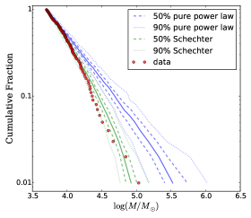
(a) Radius $<4$ kpc

(b) Radius $>4$ kpc

Figure 2: Cumulative cluster mass functions in the inner ($R_{\rm GC}<4$ kpc) and outer regions of M51. The legends are the same as in Fig. 1. (a) $M_{\text{min}}=5000$ $M_{\odot}$, $\log(M_{\star}/M_{\odot})=5$, $\beta=2$; (b) $M_{\text{min}}=5000$ $M_{\odot}$, $\log(M_{\star}/M_{\odot})=5.17$, $\beta=2$.

In Fig. 2 we show the best-fitting results for a set of Monte Carlo simulations that were similarly stochastically sampled from an underlying Schechter cluster MF as the observational data, for a power-law index $\beta=-2$. We show the results for both the inner and the outer regions of M51, adopting a radius of 4 kpc as our operational boundary. The truncation mass was chosen in the same way as for Fig. 1: $M_{\star}=1.0\times 10^{5}$ $M_{\odot}$ and $1.5\times 10^{5}$ $M_{\odot}$ for the inner and outer regions, respectively.

The masses of the most massive star clusters are well-determined, since they are not strongly affected by stochastic IMF sampling effects. However, because of stochastic IMF effects, the determination of star cluster masses based on integrated photometry may become highly uncertain for low-mass clusters (e.g., Maíz Apellániz, 2009; Fouesneau & Lançon, 2010; Anders et al., 2013; de Grijs et al., 2013, and references therein). We thus also adopt a minimum cluster mass for our cluster sample selection. The choice of the lower mass limit is important, because the presence or absence of low-mass star clusters can affect the distribution of the radial bins if the latter are selected to contain constant numbers of clusters.

When fitting the data with a Schechter function, we adopt a minimum mass of $M_{\rm cl}=5000M_{\odot}$. We conclude that reducing the low-mass limit to values much below $5000M_{\odot}$ leads to significant instability in the fits and this thus affects the eventual robustness of the parameters returned by the fits. Application of this selection limit ensures that we retain 17% of the total sample of cluster candidates (633 objects). Our simulations result in better fits than those previously obtained by both Bastian et al. (2012) and Konstantopolous et al. (2013). By comparison with the latter authors, it appears that this difference is largely caused by the differences in the adopted mass limits.

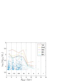
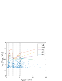
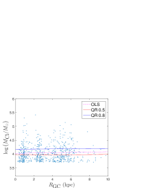
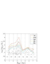
Figure 3: (a) Young M51 star cluster masses as a function of galactocentric radius, adopting a minimum mass limit of $M_{\rm cl}=10^{3}M_{\odot}$. The radial bin size adopted is 2 kpc; the numbers shown in each bin indicate the cluster numbers included. The solid lines connect the $i^{\rm th}(i=1,2,3,4,5)$ ranked most massive clusters in each bin. The effects of varying the bin sizes will be explored in Section 4.3. (b) As (a), but using radial bin sizes containing constant cluster numbers ($N=50$), as indicated by the vertical dashed lines. (c) Comparison of the results of our linear OLS fit (purple dashed line) with those resulting from QR for $\tau=0.5$ (red solid line) and $\tau=0.8$ (blue solid line), where $\tau$ refers to the $\tau^{\rm th}$ sample quartile; see Section 4. (d) As (a) but for the M83 star cluster system, adopting radial bin sizes of 1 kpc.

Figure 3a shows the distribution of the young cluster masses in M51 as a function of galactocentric radius, where the age and mass ranges have been restricted as discussed above. The clusters are grouped here in radial bins with fixed widths of 2 kpc each. The differently colored solid lines connect the $i^{\rm th}(i=1,2,3,4,5)$ ranked most massive clusters in each bin. The numbers at the bottom of each bin indicate the number of young clusters contained in the relevant bin.

There is a clear general tendency that the mass of the $i^{\rm th}$ ranked most massive cluster decreases with increasing galactocentric distance, at least out to $R_{\rm GC}\simeq 7$–8 kpc. However, the number of clusters in each bin also decreases, which signals that the observed trend may be confounded by size-of-sample effects. PA13 suggested that, at first glance, a similar result they obtained for their M33 objects may correspond to the simple, universal probability density distribution function (PDF) given by the ICMF. However, they pointed out that they cannot rule out a different model where the formation of the most massive star clusters is limited by the local physical conditions, e.g., by the local gas density (e.g., Pflamm-Altenburg & Kroupa 2008).

To further examine the physical relevance of this possibility, we tried to eliminate the size-of-sample effect by adopting radial bin sizes such that each bin contained the same number of clusters. If the ICMF represents a simple, universal, and environment-independent PDF, then we would not expect to find any radial dependence of the mass of the $i^{\rm th}$ ranked most massive star cluster. We adopted bins containing 60 clusters each for our analysis: see Fig. 3b. In each bin, we identified the $i^{\rm th}$ ranked most massive young star clusters. The galactocentric radii assigned to the $i^{\rm th}$ ranked most massive star clusters are the averages of the radial distances of all star clusters in the relevant bin.

We first used the OLS method to fit straight lines to the data,

$$\log(M_{\text{cl}}/{M_{\odot}})=aR_{\rm GC}({\text{kpc}})+b,$$ (1)

where $a$ and $b$ are the slope and intercept, respectively. Our fit results for M51 are rather different from those of PA13 for M33. The latter authors found a maximum absolute value of the slope for all clusters of 0.158 (for all data sets considering the second to the fifth most massive clusters in each bin), while for the same relative masses our maximum absolute value for the slope is merely 0.036. This difference has important implications for our understanding of the cluster-formation mode in the host galaxy. If the ICMF would be independent of its natal environment, i.e., if cluster formation were to proceed stochastically, the expected slope for the young massive clusters would be zero, modulo the size-of-sample effect. The observed value of the slope of the cluster mass–galactocentric radius relation thus becomes a useful criterion to test statistically for ICMF departures from the hypothesis of a universal (“stationary,” in statistical terms) stochastic cluster-formation process.

Table 1: Slopes of the radial distribution of the $i^{\rm th}$ ranked most massive star cluster in each bin in M51. The conditions imposed on our datasets are discussed in Section 5.

Condition	$i^{\rm th}$	Slope	Intercept	$p$ value
		($a$)	($b$)
$N=50$	1	0.045	4.8	0.26
$\log\left(M_{\rm{cl}}/M_{\odot}\right)$	2	0.028	4.7	0.081
$>3.7$;	3	0.0060	4.6	0.80
$\log(t\mbox{ yr}^{-1})$	4	$-$0.0051	4.6	0.71
$\leq 7$	5	0.0042	4.5	0.77
$N=50$	1	0.046	4.8	0.21
$\log\left(M_{\rm{cl}}/M_{\odot}\right)$	2	0.031	4.6	0.056
$>3.7$;	3	0.028	4.5	0.24
$\log(t\mbox{ yr}^{-1})$	4	$-$0.0041	4.6	0.81
$\leq 7.3$	5	0.00091	4.5	0.96
$N=50$	1	0.025	4.8	0.48
$\log\left(M_{\rm{cl}}/M_{\odot}\right)$	2	0.010	4.6	0.70
$>3.5$;	3	$-$0.0025	4.5	0.89
$\log(t\mbox{ yr}^{-1})$	4	0.0041	4.4	0.81
$\leq 7$	5	0.00067	4.4	0.97
$N=30$	1	0.037	4.7	0.29
$\log\left(M_{\rm{cl}}/M_{\odot}\right)$	2	0.0032	4.6	0.90
$>3.7$;	3	0.0078	4.5	0.65
$\log(t\mbox{ yr}^{-1})$	4	0.00094	4.4	0.95
$\leq 7$	5	$-$0.0021	4.4	0.89
$N=40$	1	0.037	4.8	0.30
$\log\left(M_{\rm{cl}}/M_{\odot}\right)$	2	0.024	4.6	0.15
$>3.7$;	3	0.036	4.5	0.050
$\log(t\mbox{ yr}^{-1})$	4	0.0033	4.5	0.75
$\leq 7$	5	0.011	4.4	0.34
$N=60$	1	0.043	4.8	0.34
$\log\left(M_{\rm{cl}}/M_{\odot}\right)$	2	0.025	4.7	0.17
$>3.7$;	3	0.020	4.6	0.39
$\log(t\mbox{ yr}^{-1})$	4	$-$0.012	4.6	0.28
$\leq 7$	5	$-$0.004	4.5	0.74

To gain a better insight into the cluster mass–galactocentric radius relation characteristic of the M51 cluster population, we next used the QR method (Koenker 2005; Feigelson & Babu 2012; Ivezić et al. 2014). QR analysis is often used in statistics and econometrics. Whereas the OLS method results in estimates that approximate the conditional mean of the response variable (in the context of the analysis of this paper, the response variable is the cluster mass) given certain values of the predictor variables (here, the galactocentric distances), QR aims at estimating either the conditional median or other quantiles of the response variable. QR estimates are more robust against outliers in the response measurements than their OLS-based counterparts. In addition, QR analysis does not impose arbitrary binning, such as that required above to bend OLS to the purpose of quantile fitting.

Symmetry implies that the minimization of the sum of the absolute residuals must be equal to the number of positive and negative residuals. Since the symmetry of the absolute values yields the median, minimizing a sum of asymmetrically weighted absolute residuals—i.e., simply giving differing weights to positive and negative residuals—yields the quantiles. We thus need to solve

$$\min\limits_{\xi\in\Re}\sum\rho_{\tau}\left(y_{i}-\xi\right),$$ (2)

where the function $\rho_{\tau}(\cdot)$ is the tilted absolute value function targeting the $\tau^{\rm th}$ sample quantile. To model a dependence of the median on a given variable and thus obtain an estimate of the conditional median function, we need to replace the scalar $\xi$ by the parametric function $\xi(x_{i},\beta)$ and adopt $\tau=\frac{1}{2}$. To obtain estimates of the other conditional quantile functions, we replace the absolute values by $\rho_{\tau}(\cdot)$ and solve

$$\min\limits_{\xi\in\Re p}\sum\rho_{\tau}\left(y_{i}-\xi(x_{i},\beta)\right).$$ (3)

When $\xi(x_{i},\beta)$ is a linear function of parameters, the resulting minimization problem can be solved very efficiently using linear programming methods.

QR examines the relation between the response variable (cluster mass) and predictor variable (galactocentric distance) for a quantile $\tau$. Unlike OLS regression, we now have a family of curves to interpret, and we can focus our attention on the particular segments of the conditional distribution, thus obtaining a more complete view of the relationship between the variables (Koenker & Hallock, 2001). Although we employ a frequentist QR approach in the present work (adapted from Koenker 2009), it is worth noting that Bayesian versions exist (e.g., Yu & Moyeed 2001), which can be readily incorporated into hierarchical models to account for complexities, such as the presence of large uncertainties in the explanatory variables.

We selected the M51 cluster sample from Fig. 1a and 1b to demonstrate the QR result. The data selection in Fig. 3c is identical to that used for the OLS regression. The red dashed line represents the linear OLS fit, while the blue and black solid lines represent the QR results for $\tau=0.5$ and $\tau=0.8$, respectively. The line pertaining to the QR result for $\tau=0.5$ has a similar intercept and slope as that resulting from the OLS regression, whereas QR for $\tau=0.8$ yields a much larger intercept, although it returns a similar slope.

Figure 5 shows the slopes as a function of $\tau$ for different age ranges. Except for the smallest regressed quantiles (where a null slope is enforced by our fixed lower mass limit), the corresponding galactocentric radius is associated, for the maximum likelihood solution, with a very small decrease in the mass distribution. Taking the standard error ($\sigma$) into account, a Wald test (Wald 1939) rules against rejection of the null hypothesis (zero slope) for all quantiles. This is so, because the approximate $3\sigma$ confidence intervals encompass a slope of zero for (almost) all quantiles. The simple frequentist $p$-value interpretation of the Wald test then automatically recommends against rejecting the null hypothesis. We point out that for a very small number of values of $\tau$, and depending on the age range considered, the Wald test cannot be applied directly. From a statistical point of view, this can be understood by realizing that the Wald test is, strictly speaking, only applicable to single quantiles, while in this case we run into non-independent multiple hypothesis testing if we are to look over all possible quantiles.

Finally, to validate our observational results for M51, we constructed a mock cluster population characterized by a Schechter-type MF. Using our simulated cluster population, we explored two conditions, one where the truncation mass does not depend on galactocentric distance and a second where the truncation in the galaxy’s inner regions occurs for cluster masses that are 2–3 times higher than those in the galactic periphery. We randomly assigned cluster ages from 5 Myr (the youngest cluster age in our observational sample) to 500 Myr, adopting a constant cluster formation rate for the entire intervening period for simplicity. We used the Bruzual & Charlot (2003) SSP models to assign $B$-band magnitudes to our sample clusters, a choice driven by the characteristics of the data set of Chandar et al. (2011), whose cluster photometry is ultimately limited by their $B$-band observations. We applied the observational magnitude limit from Chandar et al. (2011) and adjusted the number of clusters to reproduce the observational data set as closely as possible given the adopted constraints. The distributions in the diagnostic age–mass plance of both the observed M51 cluster population and our mock sample are shown in Fig. 4a and b.

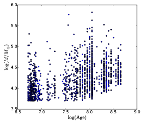
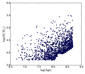
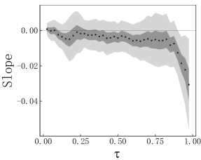
Figure 4: (a) Age–mass distribution of our observational M51 cluster sample. (b) Equivalent distribution of the simulated clusters. The magnitude limit adopted determines the number of sample clusters, while the total number of clusters above the adopted completeness limit is based on the number of clusters in our M51 sample. (c) QR result for clusters with a universal (radius-independent) truncation mass. (d) QR result for clusters characterized by a radius-dependent truncation mass.

First, we considered the cluster MFs for age ranges younger and older than $10^{8}$ yr for a universal truncation mass, $M_{\star}=10^{5}M_{\odot}$. For the younger clusters, we adopted a low-mass limit of $5000M_{\odot}$. The resulting value of $M_{\star}$ was 50% higher than expected, $M_{\star}\simeq 2\times 10^{5}M_{\odot}$. For the older cluster sample, with ages between 100 Myr and 500 Myr, we adopted a low-mass limit of $10^{4}M_{\odot}$, which resulted in a derived truncation mass of $M_{\star}\simeq 1.25\times 10^{5}M_{\odot}$. This difference in the derived truncation masses reflects the uncertainties pertaining to our calculations. The corresponding QR test for this mock data set is similar to what we found previously, resulting in a close-to-zero slope for all quantiles.

Second, we considered the case of a truncation mass that depends on galactocentric distance. Observationally, a galactocentric-distance dependence has not been established for the M51 cluster population. Therefore, we adopted Bastian et al.’s (2012) suggested radial dependence for the M83 clusters for our mock test. They reported truncation masses of $M_{\star}=2\times 10^{5}M_{\odot}$ and $M_{\star}=10^{5}M_{\odot}$ for, respectively, the inner and outer regions of the galaxy. Applying our approach to the entire cluster sample, we derive $M_{\star}\simeq 2\times 10^{5}M_{\odot}$, since the number of clusters in the galaxy’s inner regions is much larger than that at larger radii. However, considering the truncation masses for different radial ranges separately, we derived values consistent with the theoretical input values, within the method’s typical uncertainties. Thus, if the truncation mass varies systematically by a factor of 2 (or more) radially across a given galaxy, we should expect this to show up in our results. The corresponding QR test also allows us to distinguish between cluster MFs with truncation masses that differ by at least a factor of 2.

5 Parameter Dependence

In order to explore how the results depend on the adopted ICMF parameters, we varied the maximum age and minimum mass limits, as well as the radial bin size, and re-analyzed the clusters’ mass–galactocentric radius relationship. The maximum age limit adopted determines the number of clusters included in our sample; varying the maximum age limit leads to significantly different sample sizes. The minimum mass limit adopted determines the distribution of the star clusters in radial bins containing constant cluster numbers. Varying the minimum mass limit will thus change the mass and location of the most massive star cluster in each bin, which will affect our analysis pertaining to stochasticity in the ICMF. Bin-size variations also have an immediate effect on the resulting ICMF.

5.1 Maximum Age Limit

If we adopt a maximum age for the young clusters of $10^{7.3}$ yr (20 Myr), the resulting M51 cluster sample includes 689 objects. The previously noted tendency that the maximum cluster masses decrease with increasing galactocentric radius is still obvious. However, for both the OLS (adopting equal-number radial bins) and QR analyses, the resulting slopes of the linear fits tend to values close to zero. The detailed results are included in Table 1. The maximum slope for the second or third most massive cluster in each bin ranges from 0.025 to 0.036; for the first-ranked cluster in each bin, which we treat separately for stochastic reasons, the maximum slope attained ranges from 0.037 to 0.046.

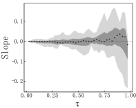
(a) $\log(t\mbox{ yr}^{-1})\leq 6.9$

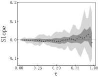
(b) $\log(t\mbox{ yr}^{-1})\leq 7.0$

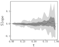
(c) $\log(t\mbox{ yr}^{-1})\leq 7.2$

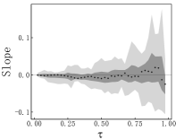
(d) $\log(t\mbox{ yr}^{-1})\leq 7.4$

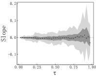
(e) $\log(t\mbox{ yr}^{-1})\leq 7.6$

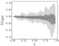
(f) $\log(t\mbox{ yr}^{-1})\leq 7.8$

Figure 5: QR results for different maximum age limits in M51, as indicated. The slope of the estimated linear QR is plotted as a function of $\tau$. Dark and light gray shading represent the $1\sigma$ and $3\sigma$ confidence intervals, respectively.

We next tested the relationship adopting a variety of maximum ages. Figure 5 shows the QR result for clusters with maximum ages spanning the range from $10^{6.9}$ yr to $10^{7.8}$ yr. In all six test conditions, the values of the maximum cluster masses appear to be functions of galactocentric radius. For small $\tau$, the slope fluctuates around 0, while for $\tau\approx 0.8$, the slopes increase. No matter the extent to which we adjust the age range, the intercept remains the same and the extent to which the slope fluctuates remains stable. A zero slope is, in all cases, contained within the $1\sigma$ range. It is thus clear that varying the upper age limit has a negligible effect on the cluster mass–galactocentric radius relation.

In addition, we point out that the uncertainty becomes rather large for $\tau\geq 0.9$. This strongly suggests that the stochastic ICMF does not depend significantly on the upper age limit adopted. As long as the clusters are sufficiently young, stochastic effects appear to average out.

5.2 Lower Mass Limit

Figure 6 is similar to Fig. 5, but for variations in the minimum cluster mass limit adopted; we varied the lower mass limit from $10^{3.3}M_{\odot}$ to $10^{3.9}M_{\odot}$ to assess the effects of sampling incompleteness. The lower mass limit adopted has a large influence on the results of our fits. In Fig. 6a, the slope deviates from 0 around the $3\sigma$ confidence level, since the lower-mass limit adopted is well below the level where our sample is statistically complete. In other cases, changing the mass limit does not change the resulting pattern significantly. In Fig. 6b, where we have adopted a lower-mass limit of $\sim 3200M_{\odot}$, the slope is consistent with a value of 0 at or within the $1\sigma$ confidence level, while Fig. 6c (for a lower-mass limit of $5000M_{\odot}$) reveals that for all values of $\tau$ the slope is consistent with zero well inside the $1\sigma$ limit. This leads us to suggest that the sample is most likely statistically complete for lower masses in the range from apprimately $3500M_{\odot}$ to $5000M_{\odot}$. Figure 6d shows the results for a lower-mass limit of $6000M_{\odot}$ as adopted by Chandar et al. (2011; their $\sim 90$% completeness limit), which may indeed be a somewhat conservative choice. Nevertheless, for reasons of consistency with previously published results, we followed Chandar et al. (2011) as regards the completeness limit adopted in this paper.

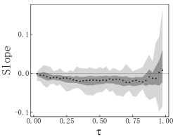
(a) $\log(M_{\rm cl}/M_{\odot})\geq 3.3$

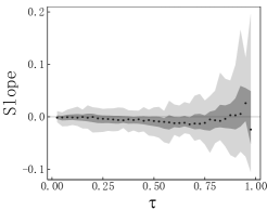
(b) $\log(M_{\rm cl}/M_{\odot})\geq 3.5$

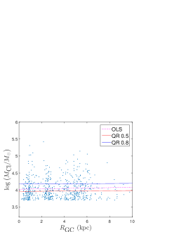
(c) $\log(M_{\rm cl}/M_{\odot})\geq 3.7$

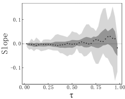
(d) $\log(M_{\rm cl}/M_{\odot})\geq 3.78$

Figure 6: As Fig. 5, but for different minimum mass limits, as indicated.

These results can be understood by considering the distribution of the lowest cluster masses as a function of distance from the center of M51. For a radial range from the galactic center out to $R\simeq 6$ kpc, and adopting bins of equal radial ranges for simplicity, the numbers of clusters with masses $\log(M_{\rm cl}/M_{\odot})\geq 3.7$ do not exhibit any significant radial trend, irrespective of the radial bin size adopted (for comparison, see Table 1; although there we included the full range in galactocentric distances covered by our sample clusters). However, if we adopt a lower-mass limit of $\log(M_{\rm cl,min}/M_{\odot})=3.3$, an overall downward radial trend becomes discernible, despite the significant fluctuations on interarm scales. Our simulations involving mock clusters lead to a similar result. If the lower-mass limit adopted is sufficiently high enough so that the level of sampling completeness is $\gtrsim 80$%, the artificial clusters can be fitted adequately with a Schechter MF. For lower completeness fractions, the fits become significantly worse.

5.3 Radial Bin-size Variations

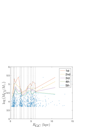
(a) $N=40$

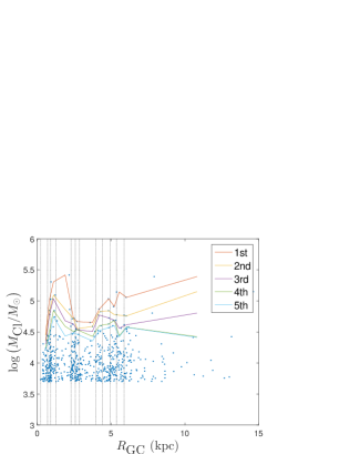
(b) $N=50$

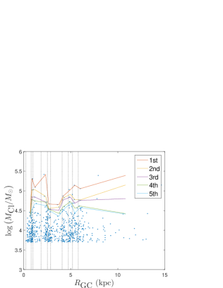
(c) $N=60$

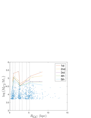
(d) $N=80$

Figure 7: OLS analysis of the M51 star cluster distribution for different radial bin sizes, with cluster numbers as indicated.

In Fig. 7, the number of clusters in each radial bin varies from 40 to 80. The slopes of the $i^{\rm th}$-ranked lines in our OLS fits have similar values (see Table 1 for details). Although we see slightly decreasing trends, the values are consistent with flat slopes, within the uncertainties. This suggests that the choice of radial bin size does not affect the results significantly.

6 The M83 Cluster Population

M83 is a barred spiral galaxy, seen on the sky in the constellation Hydra. We adopted a distance of $D=4.79$ Mpc (Karachentsev et al., 2007); the inclination and position angles were taken as $24^{\circ}$ and $45^{\circ}$, respectively (Zimmer et al., 2004).

The majority of the M83 star clusters have ages corresponding to one of two peaks, at $10^{7.2}$ and $10^{8.1}$ yr. The clusters in M83 are thus, on the whole, older than those in M51. If we only were to select clusters associated with the young peak for our analysis, we would be left with a cluster sample that is insufficiently large to obtain statistically robust results. We therefore adopted an upper age limit of $10^{8}$ yr. The masses of the M83 clusters are also higher than those in M51. Nevertheless, we still adopt a minimum mass limit of $M_{\rm cl}=5000M_{\odot}$. Figure 3d shows the radial distribution of the young massive clusters in M83.

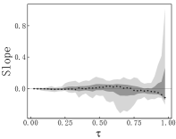
(a) $\log(t\mbox{ yr}^{-1})\leq 7.7$

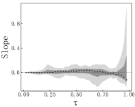
(b) $\log(t\mbox{ yr}^{-1})\leq 7.8$

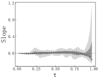
(c) $\log(t\mbox{ yr}^{-1})\leq 7.9$

(d) $\log(t\mbox{ yr}^{-1})\leq 8$

(e) $\log(t\mbox{ yr}^{-1})\leq 8.1$

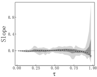
(f) $\log(t\mbox{ yr}^{-1})\leq 8.2$

Figure 8: As Fig. 5, but for the M83 cluster population.

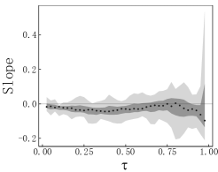
(a) $\log(M_{\rm cl}/M_{\odot})\geq 3.3$

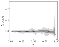
(b) $\log(M_{\rm cl}/M_{\odot})\geq 3.5$

(c) $\log(M_{\rm cl}/M_{\odot})\geq 3.7$

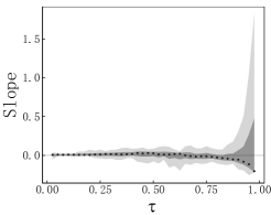
(d) $\log(M_{\rm cl}/M_{\odot})\geq 3.9$

Figure 9: As Fig. 6, but for the M83 cluster population.

Figure 8 is similar to Fig. 5. They show some common ground, although the slope decreases for large values of $\tau$; the fluctuations of the slope in M83 appear stronger than those pertaining to the M51 cluster population, particularly for the larger quantiles. Figure 9 is similar to Fig. 6. Somewhat differently from the results for M51, the fluctuation level again increases slightly for larger quantiles.

We point out that, as in Fig. 2, for a small number of values of $\tau$ in both Fig. 8 and Fig. 9, the Wald test cannot be used to rule against rejection of the null hypothesis (zero slope). Again, this can be understood by realizing that the Wald test is, strictly speaking, only applicable to single quantiles, while in this case we run into non-independent multiple hypothesis testing if we are to look over all possible quantiles.

7 The LMC Cluster Population and a Revisit of the M33 Cluster Sample

The LMC is an irregular, Magellanic-type dwarf galaxy with a prominent central bar and hints of spiral arms. We adopted a distance of $D=49.9$ Mpc (de Grijs et al., 2014). The inclination and position angles were taken as $34.7^{\circ}$ and $122.5^{\circ}$, respectively (van der Marel & Cioni, 2001). The majority of the LMC star clusters have ages corresponding to a dominant peak at $10^{8.0}$ yr. In fact, the clusters in the LMC have similar age and mass distributions as those in M83. We adopted an upper age limit of 500 Myr and a minimum mass limit of $M_{\rm cl}=5000M_{\odot}$ based on Monte Carlo tests (see Fig. 10a). This choice left us with a sample of 179 star clusters. The truncation mass in the LMC is consistent with that found by Maschberger & Kroupa (2009).

The linear fit results (see Fig. 10b) are included in Table 2. Except for the most massive clusters in each radial bin, the slopes are very small. A more in-depth analysis of the dataset shows that any relationship between cluster mass and galactocentric radius is weak. This is exemplified by the QR analysis shown in Fig. 10c.

We next decided to revisit the M33 cluster population. We extended the age range of interest to cluster ages $\lesssim 500$ Myr so as to check for environmental effects within M33, if any, on a statically sound basis. In Fig. 10d–f we show the results for this cluster sample’s best-fitting truncation mass and lower mass limit. Again, although statistically less robust than the results for either M51 or M83, the behavior of the M33 cluster population corroborates the scenario deemed most viable for those larger galaxies.

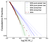
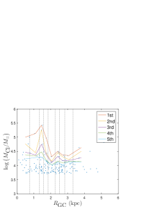
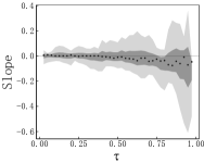
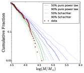
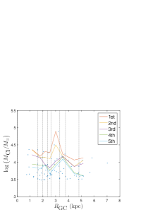
Figure 10: (a) and (d) Monte Carlo tests applied to (a) the LMC and (d) the M33 cluster samples, resulting in a best-fitting truncation mass of $6.8\times 10^{4}$ $M_{\odot}$ for a lower mass limit of $5000M_{\odot}$ in both cases. (b) and (e) OLS results based on the cluster mass–galactocentric radius distributions of the LMC cluster sample (20 clusters per radial bin) and (e) the M33 cluster population (10 clusters per radial bin). (c) and (f) QR results for the LMC and M33 cluster samples, respectively.

Table 2: Slopes of the radial distribution of the $i^{\rm th}$ ranked most massive star cluster in each bin in the LMC.

Condition	$i^{\rm th}$	Slope	Intercept	$p$ value
		($a$)	($b$)
$N=16$	1	$-$0.26	5.2	0.051
$\log\left(M_{\rm{cl}}/M_{\odot}\right)$	2	$-$0.14	4.8	0.23
$>3$;	3	$-$0.10	4.6	0.12
$\log(t\mbox{ yr}^{-1})$	4	$-$0.095	4.4	0.054
$\leq 8$	5	$-$0.058	4.3	0.092

8 Discussion and Conclusions

The high-mass regime of the ICMF and its properties have been the subject of discussions by many authors. Whether or not the ICMF is established through universal stochastic processes, on scales of individual galaxies, remains an unsolved problem, however. Young massive clusters could potentially provide good tools to check the ICMF’s dependence on its environment by means of a careful analysis of the cluster mass–galactocentric radius relation.

In this paper, we have used star cluster data from M33, M51, M83, and the LMC to examine the formation scenarios of the young massive star clusters in these galaxies. By restricting the cluster ages and masses to within certain limits, we derived the galaxies’ cluster MFs. We also explored the importance of the characteristic “truncation mass.” We first distributed the cluster samples in bins of constant galactocentric radius. Simplistic application of the OLS method resulted in a strong trend of decreasing maximum cluster mass with increasing radius. However, to eliminate size-of-sample effects, we next adopted bin sizes containing constant numbers of clusters. The trends pertaining to the first to fifth most massive clusters in each bin all but disappeared, resulting in near-zero slopes in the context of our OLS fits.

Second, we applied QR analysis to our data to examine the relation between the young cluster masses and their galactocentric distances as a function of the sample quantile, $\tau$. The quantile curves start from zero for small quantiles ($\tau<0.2$) and fluctuate for $0.2\leq\tau\leq 0.8$. For these values of $\tau$, the results are in agreement with those from the equal-number-binned OLS analysis. Both methods yield near-zero slopes (within $1\sigma$ to $3\sigma$) in the cluster mass–galactocentric radius plane. We point out that one should be careful when directly assessing any environmental dependence for large $\tau$.

We also investigated the parameter dependence on the maximum age and minimum mass imposed, as well as that on the bin size adopted. The resulting slopes do not show any strong dependence on the maximum age or bin size adopted. However, for M51, the slope decreases significantly for increasing mass limits. Based on our analysis of the star cluster populations in M33, M51, M83, and the LMC, we find that the star cluster mass–galactocentric radius dependence is similar for all four host galaxies, within the prevailing uncertainties. This implies that star cluster formation does not necessarily require an environment-dependent cluster formation scenario, which thus supports the notion of stochastic star cluster formation as dominant cluster-formation process (see Gieles et al. 2006; Gieles 2009), at least within a given galaxy.

References

- Adamo & Bastian (2015) Adamo, A., & Bastian, N. 2015, in: The Birth of Star Clusters, ed. S. W. Stahler, New York, NY: Springer, in press
- Adamo et al. (2010a) Adamo, A., Östlin, G., Zackrisson, E., et al. 2010, MNRAS, 407, 870
- Adamo et al. (2010b) Adamo, A., Zackrisson, E., Östlin, G., & Hayes, M. 2010, ApJ, 725, 1620
- Anders et al. (2004) Anders, P., Bissantz, N., Fritze-v. Alvensleben, U., & de Grijs, R. 2004, MNRAS, 347, 196
- Anders & Fritze-v. Alvensleben (2003) Anders, P., & Fritze-v. Alvensleben, U. 2003, A&A, 401, 1063
- Anders et al. (2013) Anders, P., Kotulla, R., de Grijs, R., & Wicker, J. 2013, ApJ, 778, 138
- Bastian (2008) Bastian, N. 2008, MNRAS, 390, 759
- Bastian et al. (2011) Bastian, N., Adamo, A., Gieles, M., et al. 2011, MNRAS, 417, 6
- Bastian et al. (2005) Bastian, N., Gieles, M., Lamers, H. J. G. L. M., Scheepmaker, R. A., & de Grijs, R. 2005, A&A, 431, 905
- Baumgardt et al. (2013) Baumgardt, H., Parmentier, G., Anders, P., & Grebel, E. K. 2013, MNRAS, 430, 676
- Bik et al. (2003) Bik, A., Lamers, H. J. G. L. M., Bastian, N., Panagia, N., & Romaniello, M. 2003, A&A, 397, 473
- Bruzual & Charlot (2003) Bruzual, G., & Charlot, S. 2003, MNRAS, 344, 1000
- Cameron (2013) Cameron, E. 2013, https://astrostatistics.wordpress.com/2013/12/01/bordering-on-scientific-misconduct/ Accessed: 28 August 2015
- Chandar et al. (2010) Chandar, R., Whitmore, B. C., Kim, H., et al. 2010, ApJ, 719, 966
- Chandar et al. (2011) Chandar, R., Whitmore, B. C., Calzetti, D., et al. 2011, ApJ, 727, 88
- de Grijs et al. (2003) de Grijs, R., Anders, P., Bastian, N., et al. 2003, MNRAS, 343, 1285
- de Grijs et al. (2005) de Grijs, R., Anders, P., Lamers, H. J. G. L. M., et al. 2005, MNRAS, 359, 874
- de Grijs et al. (2013) de Grijs, R., Anders, P., Zackrisson, E., & Östlin, G. 2013, MNRAS, 431, 2917
- de Grijs et al. (2014) de Grijs, R., Wicker, J. E., & Bono, G. 2014, AJ, 147, 122
- Fall & Chandar (2012) Fall, S. M., & Chandar, R. 2012, ApJ, 752, 96
- Fan & de Grijs (2014) Fan, Z., & de Grijs, R. 2014, ApJS, 211, 22
- Feigelson & Babu (2012) Feigelson, E. D., & Babu, G. L. 2012, Modern Statistical Methods for Astronomy: With R Applications. Cambridge, UK: CUP
- Feldmeier et al. (1997) Feldmeier, J. J., Ciardullo, R., & Jacoby, G. H. 1997, ApJ, 479, 231
- Fouesneau & Lançon (2010) Fouesneau, M., & Lançon, A. 2010, A&A, 521, A22
- Gieles (2009) Gieles, M. 2009, Ap&SS, 324, 299
- Gieles et al. (2006) Gieles, M., Larsen, S. S., Scheepmaker, R. A., et al. 2006, A&A, 446, L9
- Glatt et al. (2010) Glatt, K., Grebel, E. K., & Koch, A. 2010, A&A, 517, 50
- Ivezic et al. (2014) Ivezić, Z., Connolly, A., Vanderplas, J., & Gray, A. 2014, Statistics, Data Mining and Machine Learning in Astronomy, Princeton, NJ: Princeton Univ. Press
- Karachentsev et al. (2007) Karachentsev, I. D., Tully, R. B., Dolphin, A., et al. 2007, AJ, 133, 504
- Koenker (2005) Koenker, R. 2005, Quantile Regression (Econometric Society Monographs), Cambridge, UK: CUP
- Koenker (2009) Koenker, R. 2009, quantreg: Quantile Regression. R package version 4.27. http://CRAN.R-project.org/package=quantreg
- Koenker & Hallock (2001) Koenker, R. & Hallock, K. F. 2001, J. Econ. Perspect., 4, 143
- Konstantopoulos et al. (2010) Konstantopoulos, I. S., Gallagher, S. C., Fedotov, K., et al. 2010, ApJ, 723, 197
- Konstantopoulos et al. (2013) Konstantopoulos, I. S., Smith, L. J., Adamo, A., et al. 2013, AJ, 145, 137
- Larsen (2009) Larsen, S. S. 2009, A&A, 494, 539
- Mackey & Gilmore (2003) Mackey, A. D., & Gilmore, G. F. 2003, MNRAS, 338, 85
- Maíz Apellániz (2009) Maíz Apellániz, J. 2009, ApJ, 699, 1938
- Maschberger & Kroupa (2009) Maschberger, T., & Kroupa, P. 2009, MNRAS, 395, 931
- Massey (2002) Massey, P. 2002, ApJS, 141, 81
- McCrady & Graham (2007) McCrady, N., & Graham, J. R. 2007, ApJ, 663, 844
- Milone et al. (2009) Milone, A. P., Bedin, L. R., Piotto, G., & Anderson, J. 2009, A&A, 497, 755
- Moustakas et al. (2010) Moustakas, J., Kennicutt, R. C., Jr., Tremonti, C. A., et al. 2010, ApJS, 190, 233