Solving Jigsaw Puzzles with Linear Programming

Abstract

We propose a novel Linear Program (LP) based formulation for solving jigsaw puzzles. We formulate jigsaw solving as a set of successive global convex relaxations of the standard NP-hard formulation, that can describe both jigsaws with pieces of unknown position and puzzles of unknown position and orientation. The main contribution and strength of our approach comes from the LP assembly strategy. In contrast to existing greedy methods, our LP solver exploits all the pairwise matches simultaneously, and computes the position of each piece/component globally. The main advantages of our LP approach include: (i) a reduced sensitivity to local minima compared to greedy approaches, since our successive approximations are global and convex and (ii) an increased robustness to the presence of mismatches in the pairwise matches due to the use of a weighted L1 penalty. To demonstrate the effectiveness of our approach, we test our algorithm on public jigsaw datasets and show that it outperforms state-of-the-art methods.

1 Introduction

Jigsaw puzzles were first produced as a form of entertainment around 1760s by a British mapmaker and remain one of the most popular puzzles today. The goal is to reconstruct the original image from a given collection of pieces. Although introduced as a game, this problem has also attracted computer scientists. The first computational approach to solve this problem dates back to 1964 [7]. It was later shown that this combinatorial problem is NP-hard [1, 6]. Solving jigsaw puzzles computationally remains a relevant and intriguing problem noted for its applications to real-world problems. For instance the automatic reconstruction of fragmented objects in 3D is of great interest in archaeology or art restoration, where the artefacts recovered from sites are often fractured. This problem has attracted significant attention from the computer graphics community, where solutions have been offered to the automatic restoration of frescoes [9] or the reassembly of fractured objects in 3D [10].

The sustained interest in this problem has led to significant progress in automatic puzzle solvers [8, 14, 15, 16]. An automatic solver typically consists of two components: the estimation of pairwise compatibility measures between different pieces, and the assembly strategy. Most research has been dedicated to finding better assembly strategies and we continue this trend. Existing approaches tend to use either greedy strategies or heuristic global solvers, e.g. genetic algorithms. While greedy methods are known to be sensitive to local minima, the performance of genetic algorithms heavily relies on the choice of fitness function and crossover operation.

In common with the majority of works on solving jigsaw puzzles in the vision community, we focus on the difficult case in which all pieces are square, so no information about location or orientation is provided by the pieces, and the jigsaw must be solved using image information alone.

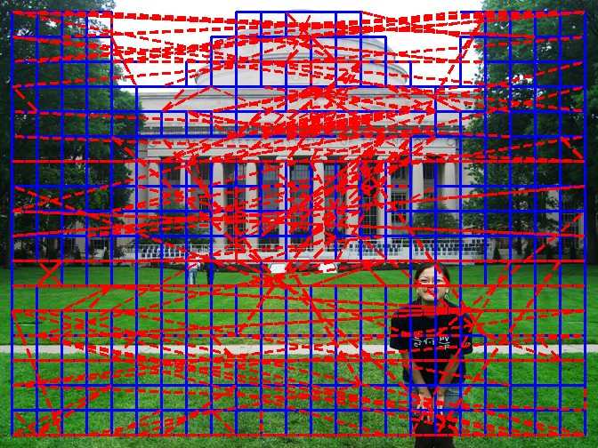
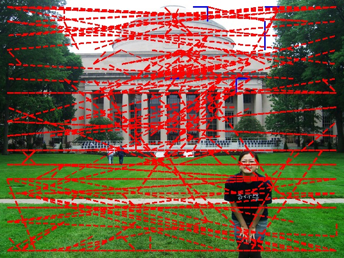
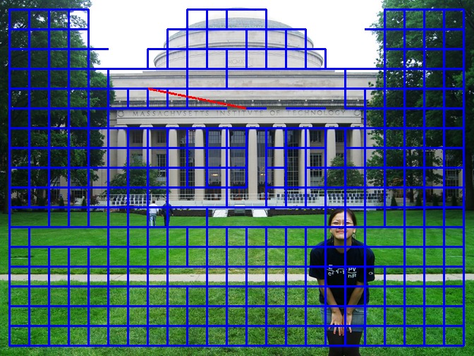
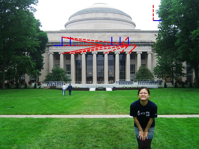
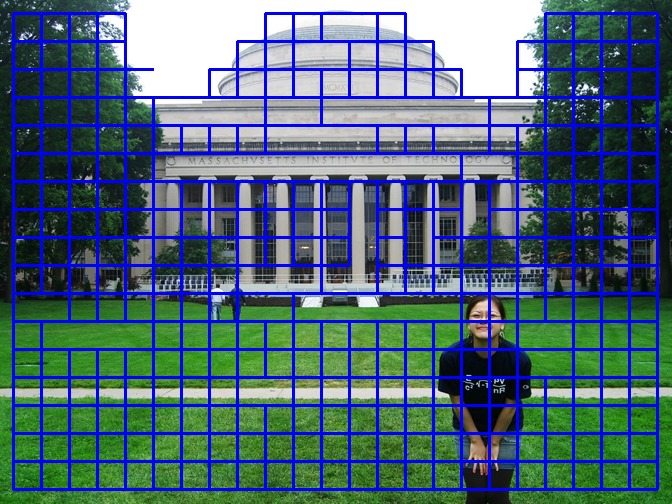
In this paper we propose a novel Linear Program (LP) based assembly strategy. We show that this LP formulation is a convex relaxation of the original discrete non-convex jigsaw problem. Instead of solving the difficult NP-hard problem in a single optimization step, we introduce a sequence of LP relaxations (see figure 1). Our approach proceeds by alternating between computing new soft constraints that may be consistent with the current LP solution and resolving and discarding this family of constraints with an LP. Starting with an initial set of pairwise matches, the method increasingly builds larger and larger connected components that are consistent with the LP.

Our LP formulation naturally addresses the so called Type 1 puzzles [8], where the orientation of each jigsaw piece is known in advance and only the location of each piece is unknown. However, we show that our approach can be directly extended to the more difficult Type 2 puzzles, where the orientation of the pieces is also unknown, by first converting it into a Type 1 puzzle with additional pieces.

2 Related Work

Initial confident pairwise matches $A^{(0)}$	Rejected matches $R^{(0)}$	Confident matches consistent with first LP $A^{(0)}-R^{(0)}$	(c) New matches introduced in second LP $A^{(1)}-A^{(0)}$	(d) Confident matches consistent with second LP $A^{(1)}-R^{(1)}$

Figure 1: Top: An example run through of the algorithm. Bottom: How bad matches are successively eliminated over the same sample run resulting in a better LP. Blue indicates correct ground-truth matches, while red indicates false. Through-out the run various low confident matches between pieces of sky are present but ignored by the algorithm due to their extremely low weight. For clarity,these are not plotted. See section 3.4.

The first automatic jigsaw solver was introduced by Freeman and Garder [7] who proposed a $9$-piece puzzle solver, that only made use of shape information, and ignored image data. This was followed by further works [18, 17] that only made use of shape information. Kosiba [11] was the first to make use of both shape and appearance information in evaluating the compatibility between different pieces.

Although it is widely known that jigsaw puzzle problems are NP-hard when many pairs of pieces are equally likely a priori to be correct [6], many methods take advantage of the unambiguous nature of visual images to solve jigsaws heuristically. Existing assembly strategies can be broadly classified into two main categories: greedy methods [8, 16, 19] and global methods [4, 2, 14, 15]. The greedy methods start from initial pairwise matches and successively build larger and larger components, while global methods directly search for a solution by maximizing a global compatibility function.

Gallagher [8] proposed a greedy method they refer to as a “constrained minimum spanning tree” based assembly which greedily merges components while respecting the geometric consistence constraints. In contrast, Son et al. [16] showed that exploiting puzzle cycles, e.g. loop constraints between the pieces, rather than avoiding them in tree assembly [8], leads to better performance. They argued that loop constraints could effectively eliminate pairwise matching outliers and therefore a better solution could be found by gradually establishing larger consistent puzzle loops. These loop constraints are related to the loop closure and cycle preservation constraints used in SLAM [5] and structure from motion [3]. Global approaches include Cho et al. [4] who formulated the problem in as a Markov Random Field and proposed a loopy belief propagation based solution. Sholomon [14, 15] has shown that genetic algorithms could be successfully applied to large jigsaw puzzles, and Andalo et al.  [2] proposed a Quadratic Programming based jigsaw puzzle solver by relaxing the domain of permutation matrices to doubly stochastic matrices.

Our approach can be seen as a hybrid between global and greedy approaches, designed to capture the best of both worlds. Unlike global approaches which can be hampered by a combinatorial search over the placement of ambiguous pieces, like greedy methods, we delay the placing of these pieces until we have information that makes their position unambiguous. However, unlike greedy methods, at each step of the algorithm, we consider the placement of all pieces, rather than just a small initial set of pieces in deciding whether a match is valid. This makes us less likely to “paint ourselves into a corner” with early mistakes. Empirically, the results presented in section 4 reflect this, and we outperform all other approaches.

3 Our Puzzle Solver

In this section we discuss the two principal components of our puzzle solver: (i) the estimation of pairwise matching costs based on image intensity information and (ii) the assembly strategy. The fundamental contribution of our work is a novel LP based assembly algorithm. After generating initial pairwise matching scores for all possible pairs of pieces at all four orientations using Gallagher’s approach [8], our algorithm solves a set of successive globally convex LP relaxations. We initially focus the description of our algorithm in the case of Type 1 puzzles where only the position of the pieces is unknown. We will then show how Type 2 puzzles can be solved by converting them into a mixed Type 1 puzzle containing copies of each piece in each of the four possible orientations.

$o=1$	$o=2$	$o=3$	$o=4$
$j$ $i$	$i$$j$	$i$ $j$	$j$$i$

Figure 2: Four different configurations for an oriented pair of matching pieces $(i,j,o)$. In this paper we assume that the positive $x$ axis points right while the positive $y$ direction points down. From left to right the orientation takes values $o=\{1,2,3,4\}$ respectively.

3.1 Matching Constraints

As shown in Figure 2, given an oriented pair of matching jigsaw pieces $(i,j,o)$ there are $4$ different possibilities for their relative orientation $o$. Accordingly, we define $4$ matching constraints on their relative positions on the puzzle grid $(x_{i},y_{i})$ and $(x_{j},y_{j})$, where $x_{i}$ and $y_{i}$ indicate the horizontal and vertical positions of piece $i$. We define the desired offsets $\delta^{x}_{o}$, $\delta^{y}_{o}$ between two pieces in $x$ and $y$ for an oriented pair $(i,j,o)$ as

$$\delta^{x}_{o}=\begin{cases}0&\quad\text{if $o=1$}\\ -1&\quad\text{if $o=2$}\\ 0&\quad\text{if $o=3$}\\ 1&\quad\text{if $o=4$}\\ \end{cases}$$

$$\delta^{y}_{o}=\begin{cases}1&\quad\text{if $o=1$}\\ 0&\quad\text{if $o=2$}\\ -1&\quad\text{if $o=3$}\\ 0&\quad\text{if $o=4$}\\ \end{cases}$$

3.2 Pairwise Matching Costs

To measure the visual compatibility between pairs of jigsaw pieces, we use the Mahalanobis Gradient Compatibility (MGC) distance proposed by Gallagher [8] which penalizes strong changes in image intensity gradients across piece boundaries by encouraging similar gradient distributions on either side. This pairwise matching cost is widely used by other authors, and therefore allows for a direct comparison of our assembly strategy against competing approaches [8, 16]. We define $D_{ijo}$ to be the MGC distance (see [8] for full definition) between pieces $i$ and $j$ with orientation $o$ (see figure 2). The matching weight $w_{ijo}$ associated with the oriented pair $(i,j,o)$ can now be computed as

$$w_{ijo}=\frac{\min(\min_{k\neq i}(D_{kjo}),\min_{k\neq j}(D_{iko}))}{D_{ijo}},$$ (1)

i.e. the inverse ratio between $D_{ijo}$ and the best alternative match. Note that these weights are large when the matching distance between pieces is relatively small and vice-versa.

3.3 NP hard objective

Input : Scrambled jigsaw puzzle pieces

Output : Assembled image

Initialisation: Generate initial pairwise matches $U^{(0)}$

1 Compute $A^{(0)}$ according to eq (14)

2 Solve (16) to get the initial solution ${\bf x}^{(0)}$, ${\bf y}^{(0)}$

3 while not converged do

4       Generate Rejected Matches $R^{(k)}$ using eq (17)

5       Update $U^{(k)}$ by discarding $R^{(k)}$

6       Compute pairwise matches $A^{(k)}$ according to eq (14)

7       Solve (16), get new solution ${\bf x}^{(k)},{\bf y}^{(k)}$

8      

end Trim and fill as necessary to get rectangular shape [8]

Algorithm 1 LP based Type 1 jigsaw puzzle solver

Given the entire set of puzzle pieces $V=\{i\mid i=1,\ldots,N\times M\}$, where $M$ and $N$ are the dimensions of the puzzle, we define the set $U=\{(i,j,o),\,\forall i\in V,\,\forall j\in V,\,\forall o\in\{0,1,2,3\}\}$ as the universe of all possible oriented matches $(i,j,o)$ between pieces (see figure (2)). Each oriented match $(i,j,o)$ will have an associated confidence weight $w_{ijo}$.

We now define the following weighted $L_{0}$ costs

$$C({\bf x})=\sum_{(i,j,o)\in U}w_{ijo}|x_{i}-x_{j}-\delta^{x}_{o}|_{0},$$ (2)

$$C({\bf y})=\sum_{(i,j,o)\in U}w_{ijo}|y_{i}-y_{j}-\delta^{y}_{o}|_{0},$$ (3)

and formulate the jigsaw puzzle problem as

minimize: $$C({\bf x})+C({\bf y})$$ (4)

subject to: $$\forall i,x_{i}\in\mathbb{N},1\leq x_{i}\leq M$$ (5)

$$\forall j,y_{j}\in\mathbb{N},1\leq y_{j}\leq N$$ (6)

$$\forall i,\forall j,\left|x_{i}-x_{j}\right|+\left|y_{i}-y_{j}\right|>0$$ (7)

where $x_{i}$ and $y_{i}$ are the $x$ and $y$ position of piece $i$ and ${\bf x}=[x_{1},x_{2},\ldots x_{n}]$, ${\bf y}=[y_{1},y_{2},\ldots y_{n}]$, with $n$ being the total number of pieces.

The objective function (4) is the sum of cost over $x$ and $y$ dimensions. The first two constraints (5, 6) are integer position constraints, that force each piece to lie on an integer solution inside the puzzle domain. The final constraint (7) guarantees that no two pieces are located in the same position. Problem (4) can be explained as searching for a configuration of all the pieces which gives the minimum weighted number of incorrect matches. However, both the feasible region and the objective (4) are discrete and non-convex, and the problem is NP-hard.

Table 1: Reconstruction performance on Type 1 puzzles from the Olmos[12] and Pomeranz[13] datasets. The size of each piece is P = 28 pixels. See Section 4 for a definition of the error measures.

	540 pieces		805 pieces		2360 pieces		3300 pieces
	Direct	Nei.	Direct	Nei.	Direct	Nei.	Direct	Nei.
Pomeranz et al. [13]	83%	91%	80%	90%	33%	84%	80.7%	95.0%
Andalo et al. [2]	90.6%	95.3%	82.5%	93.4%	-	-	-	-
Sholomon et al. [14]	90.6%	94.7%	92.8%	95.4%	82.7%	87.5%	65.4%	91.9%
Son et al. [16]	92.2%	95.2%	93.1%	94.9%	94.4%	96.4%	92.0%	96.4%
Constrained	94.0%	96.8%	95.4%	96.6%	94.9%	97.6%	94.1%	97.5%
Free	94.6%	97.3%	94.2%	96.4%	94.9%	97.6%	93.9%	97.1%
Hybrid	94.8%	97.3%	95.2%	96.6%	94.9%	97.6%	94.1%	97.5%

Table 2: Reconstruction performance on Type 2 puzzles from the Olmos and Pomeranz dataset. Each piece is a 28 pixel square. Note that our slightly worse performance than Son et al. in 3300 piece jigsaws comes from poor resolution of a patch of sky in a single image. See Section 4 for a definition of the error measures.

	540 pieces		805 pieces		2360 pieces		3300 pieces
	Direct	Nei.	Direct	Nei.	Direct	Nei.	Direct	Nei.
Son et al. [16]	89.1%	92.5%	86.4%	88.8%	94.0%	95.3%	89.9%	93.4%
Constrained	92.6%	93.1%	91.2%	92.0%	94.4%	95.5%	88.4%	89.2%
Free	88.0%	89.1%	91.4%	92.5%	94.4%	94.8%	89.7%	90.2%
Hybrid	92.8%	93.3%	91.7%	92.9%	94.4%	95.5%	89.7%	90.2%

3.4 LP based Puzzle Assembly

Figure 1 and Algorithm 1 gives overviews of our approach. The method takes scrambled pieces as input and returns an assembled image. Instead of solving the difficult puzzle problem in a single optimization step, we propose to solve a sequence of LP convex relaxations. Our approach is an incremental strategy: starting with initial pairwise matches, we successively build larger connected components of puzzle pieces by iterating between LP optimization and generating new matches by deleting those that are inconsistent with the current LP solution and proposing new candidates not yet shown to be inconsistent.

In comparison to previous greedy methods [8, 16], our approach has two main advantages. The first one is that instead of gradually building larger components in a greedy way, our LP step exploits all the pairwise matches simultaneously. The second advantage is that due to the weighted $L_{1}$ cost function, LP is robust to incorrect pairwise matches. Son et al. [16] has shown that verification of loop constraints significantly improves the precision of pairwise matches, and our work can be considered as a natural generalisation of these loop constraints that allows loops of all shapes and sizes, not necessarily rectangular, to be solved in a single LP optimization. The rest of this section describes in detail the two main components of our formulation: (i) the initial LP formulation for the scrambled input pieces, and (ii) the successive LPs for the connected components. See Figure 1 for an illustration of the whole process on an image taken from the MIT dataset.

3.4.1 LP Formulation for Scrambled Pieces

To make the problem convex, we discard the integer position constraints (5,6) and the non-collision constraints (7) and relax the non-convex $L_{0}$ norm objective to its tightest convex relaxation $L_{1}$ norm. This gives the objective

$$C^{*}({\bf x},{\bf y})= C^{*}({\bf x})+C^{*}({\bf y})$$ (8)

$$= \sum_{(i,j,o)\in U}w_{ijo}|x_{i}-x_{j}-\delta^{x}_{o}|_{1}$$ (9)

$$+ \sum_{(i,j,o)\in U}w_{ijo}|y_{i}-y_{j}-\delta^{y}_{o}|_{1}$$ (10)

In practice, this relaxation does not give rise to a plausible solution as the $L_{1}$ norm acts in a similar way to the weighted median, and results in a compromised solution that overly favours weaker matches. Instead we consider the same objective over an active subset of candidate matches $A\subseteq U$.

$$C^{+}({\bf x},{\bf y})= C^{+}({\bf x})+C^{+}({\bf y})$$ (11)

$$= \sum_{(i,j,o)\in A}w_{ijo}|x_{i}-x_{j}-\delta^{x}_{o}|_{1}$$ (12)

$$+ \sum_{(i,j,o)\in A}w_{ijo}|y_{i}-y_{j}-\delta^{y}_{o}|_{1}$$ (13)

Note that if $A$ was chosen as the set of ground-truth neighbors, solving this LP would return the solution to the jigsaw, and so finding the optimal set $A$ is N.P. hard. Instead we propose a sequence of estimators of $A$, which we write as $A^{(k)}$. In practice, throughout the LP formulation, we consider two sets of matches $U^{(k)}$ and $A^{(k)}$ for each LP iteration $k$. The first set $U^{(k)}$ begins as the universal set of all possible candidate matches for all orientations and choices of piece $U^{(0)}=U$ and is of size $4n^{2}$. In subsequent iterations of our algorithm, its $k^{\text{th}}$ form $U^{(k)}$ steadily decreases in size as our algorithm runs and rejects matches. The second set of matches $A^{(k)}$ is the active selection at iteration $k$ of best candidate matches taken from $U^{(k)}$. For all iterations, $A^{(k)}$ is always of size $4n$ and can be computed as

$$A^{(k)}=\{(i,j,o)\in U^{(k)}:j=\operatorname*{arg\,min}_{j:(i,j,o)\in U^{(k)}}D_{ijo}\},$$ (14)

We take advantage of the symmetry between $C^{+}({\bf x})$ and $C^{+}({\bf y})$, and only illustrate in the paper how to solve the $x$ coordinate subproblem.

The minimiser of $C^{+}({\bf x})$ can be written as

$${\operatorname*{arg\,min}_{\bf x}}\sum_{(i,j,o)\in A^{(k)}}w_{ijo}|x_{i}-x_{j}-\delta^{x}_{o}|_{1}.$$ (15)

By introducing auxiliary variables ${\bf h}$, we transform the minimisation of (15) into the following linear program

$${\operatorname*{arg\,min}_{{\bf x},{\bf h}}} \sum_{(i,j,o)\in A^{(k)}}w_{ijo}h_{ijo}$$ (16)

subject to $$h_{ijo}\geq x_{i}-x_{j}-\delta^{x}_{o}, (i,j,o)\in A^{(k)}$$

$$h_{ijo}\geq-x_{i}+x_{j}+\delta^{x}_{o}, (i,j,o)\in A^{(k)}.$$

Given the LP solution, we can recover the image based on the relative position of all the pieces. However, as the linear program does not enforce either integer location or collision constraints, pieces may not be grid aligned and the solution may also contain holes (no pieces in the corresponding position) or collisions (two or more pieces assigned to the same position). In practice, unlike most other convex regularizers such as $L_{2}^{2}$, the $L_{1}$ norm encourages a ‘winner takes all’ solution, and while the absolute location of each piece is arbitrary, the relative locations between adjacent pieces are very close to integers ($<10e{-6}$). Holes and collisions between pieces mostly happen where sufficiently ambiguous matches lead to fully disconnected regions, or contradictory cues lead to a region being pulled apart, with the weakest matches broken.

Generally, solving this LP does not give rise to a complete and fully aligned jigsaw. Instead we build on the solution found and by iteratively solving a sequence of LP optimizations gradually create larger and larger recovered components. As the LP robustly detects and eliminates mismatches, the matches consistent with the current LP solution can be used to establish accurate connected components of jigsaw pieces.

3.4.2 Successive LPs and Removal of Mismatches

After the $k^{th}$ LP iteration, we validate the solution and remove matches from the set $A^{(k)}$ that are inconsistent with the solution to the LP

$$R^{(k)}=\{\forall(i,j,o)\in A^{(k)}:|x_{i}-x_{j}-\delta^{x}_{o}|>10^{-5}\}.$$ (17)

We set

$$U^{(k)}=U^{({k-1})}-R^{(k)},$$ (18)

and estimate $A^{(k)}$ according to equation (14). This procedure is guaranteed to converge. Matches are only ever removed from $U^{(k)}$, and as $U^{(0)}$ is finite, the procedure must eventually stop. In practice, we never observed the algorithm take more than 5 iterations, and typically it converges after two iterations.

3.4.3 Completing the solution

Much like other methods [8, 16], the solution found is not guaranteed to be rectangular, and may still have some pieces we have been unable to assign. As such, we make use of the same post-processing of Gallagher[8], to generate a complete rectangular solution.

3.5 Constrained variants of our approach

In practice, one limitation of the above method is that the updating of $A^{(k)}$ can tear apart previously found connected components. In some cases this is good as it allows for the recovery from previously made errors but it is roughly as likely to break good components as bad.

As such, we evaluate a constrained variant of our approach, that enforces as a hard constraint that all pieces lying in a connected components must remain in the same relative position to other pieces in the component. In section 4, we evaluate these two methods and another that selects the best solution found by these two methods based on how well it minimizes the original cost $C({\bf x})+C({\bf y})$. A comparison between all three strategies can be seen in the tables of section 4, where we refer to the three approaches as free, constrained, or hybrid respectively.

(a)	(b)	(c)	(d)

Figure 3: Reconstruction results from the initial LP and our complete method, images from the MIT dataset. (a) the input pieces, (b) the largest connected component before filling, (c) the final result and (d) ground truth.

Figure 4: Example reconstruction results of Type 2 Puzzle. From left to right: the rotated input puzzle pieces, and four recovered images generated by converting to a mixed Type 1 puzzle.

Figure 5: Reconstruction on mixed Type 2 puzzle (864 mixed pieces based on two images from MIT dataset.)

Son et al. [16]	Ours

Figure 6: Comparison of Type 2 puzzle reconstruction results between our approach and Son et al. [16]. Examples are selected from MIT dataset.

3.5.1 Type 2 Puzzles

To solve the more challenging Type 2 puzzles, where both the position and orientation of the pieces is unknown, we first convert the problem into a larger Type 1 puzzle by replicating each piece with all 4 possible different rotations and then solving the four mixed Type 1 puzzles simultaneously.

The only difference with the Type 1 puzzle solver is that in this case we have an additional constraint: identical pieces with different rotations must not be assigned to the same connected component. Since this constraint is non-convex it cannot be imposed in the LP directly. In practice, we take the piece with the largest pairwise matching confidence weight and fix the positions of its four rotated versions in the LP to predefined values (in this work we place the 4 copies of the piece at $[\pm 10e{+4},\pm 10e{+4}]$). This ensures that these copies can not belong to the same connected component.

4 Experiments

To demonstrate the performance of our method, we apply our algorithm to five different datasets. The MIT dataset, collected by Cho et al. [4], contains 20 images with $432$ pieces, each with pixel size $28\times 28$. The other four datasets, due to Olmos et al. [12] and Pomeranz et al. [13], include two with 20 images ($540$ and $805$ pieces) and two with 3 images ($2360$ and $3300$ pieces).

The metric we use to evaluate our approach follows those of Gallagher [8] where four measures are computed: “Direct comparison” measures the percentage of pieces that are in the correct position, compared with the ground truth; “Neighbor comparison” measures the percentage of correct piecewise adjacencies; “Largest Component” is the fraction of pieces in the largest connected component with correct pairwise adjacencies, and “Perfect Reconstruction” is a binary measure of if all the pieces in the puzzle are in the correct position and with the correct orientation.

Type 1 Puzzles: We evaluate our approach on a wide variety of existing datasets. Table 1 shows the comparison results of our algorithm with the two state of the art methods, Gallagher [8] and Son [16] on the Pomeranz and Olmos datasets. The scores reported are the average results over all the images in each set. Our proposed approach outperforms Son et al. [16] who had previously shown that their method was state of the art compared with competing approaches. We believe that the improvements over previous methods comes from our LP assembly strategy. Compared with existing approaches, the global LP formulation and the robustness of weighted $L_{1}$ cost allows us to discard mismatches and delay the placing of ambiguous pieces leading to better performance.

The MIT dataset (Table 3) is more saturated but we still outperform all known methods. By adding noise to the images (Figure 7) the advantage of our approach over other greedier methods becomes more apparent.

Table 3: Reconstruction performance on Type 1 puzzles from the MIT dataset, The number of pieces is K = 432 and the size of each piece is P = 28 pixels. The errors reported here for Initial LP and Successive LP treat pieces that do not belong to the largest connected component as errors. As intermediate results need not be rectangular, scores are created by sliding the biggest connected component across the ground truth image and finding best matching locations.

	Direct	Neighbor	Comp.	Perfect
Cho et al. [4]	10 %	55%	-	0
Yang et al. [19]	69.2 %	86.2 %	-	-
Pomeranz et al. [13]	94 %	95 %	-	-
Andalo et al. [2]	91.7%	94.3 %	-	-
Gallagher [8]	95.3%	95.1%	95.3%	12
Sholomon et al. [14]	80.6 %	95.2%	-	-
Son et al. [16]	95.6%	95.5%	95.5%	13
Initial LP	95.1%	94.7%	95.1%	13
Successive LPs (constrained)	95.7%	95.5%	95.7%	14
Constrained	95.7%	95.7%	95.7%	14
Free	95.8%	95.6%	95.8%	14
Hybrid	95.7%	95.7%	95.7%	14
Upper Bound [16]	96.7%	96.4%	96.6%	15

Table 4: Reconstruction performance on Type 2 puzzles from the MIT dataset, The number of pieces is K = 432. Each piece is a 28 pixel square.

	Direct	Neighbor	Comp.	Perfect
Gallagher  [8]	82.2%	90.4%	88.9%	9
Son et al. [16]	94.7%	94.9%	94.6%	12
Constrained	95.6%	95.3%	95.6%	14
Free	95.6%	95.3%	95.6%	14
Hybrid	95.6%	95.3%	95.6%	14

Figure 7: Comparison of our approach vs Gallagher [8] and Son et al. [16] with different amounts of image noise. The X axis shows the standard deviation of the Gaussian noise added to the image intensity (intensities range from 0 to 65535). The Y axis shows the scores on the four performance measures. Results are averaged over five runs, and as such the number of perfect images may be non-integer.

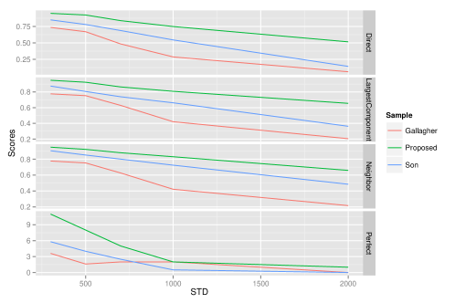
Table 3, and Tables 1 and 2 in the suplementary materials), show the performance of various components of our method. Looking at Table 1 in the suplementary materials, it can clearly be seen that our proposed approach, a sequence of LP relaxations, generates an near perfect solution (all the three metrics are very close to 100%) with most of the errors coming from the final filling step, in which ambiguous pieces must be placed to finish the assembly.

Type 2 Puzzles: As discussed in section $3$, we convert Type 2 puzzles into a mixed Type 1 puzzles (mixed by four different rotation identical images). Figure 4 shows a perfect Type 2 puzzle reconstruction from the MIT dataset. Table 4 gives the comparison results of our method with Son et al. [16] and Gallagher [8] on the MIT dataset. It can be seen that our approach consistently outperforms both methods. Table 2 shows the results on other four additional datasets, where we out-perform Son et al. [16], on all except the last dataset (which only contains three images).

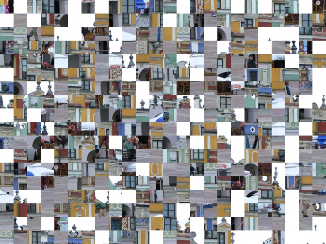
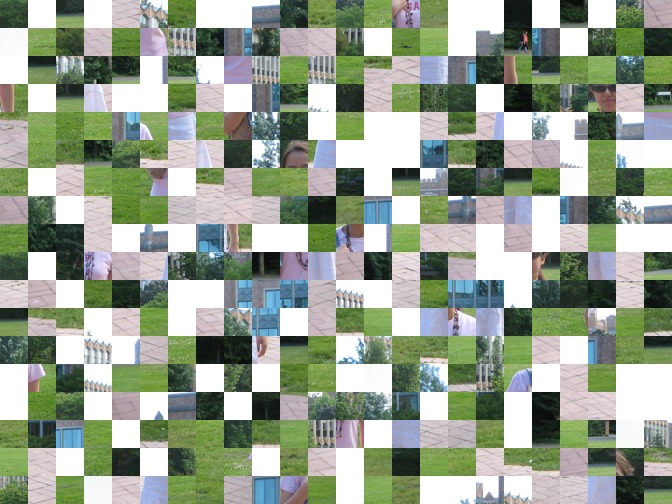
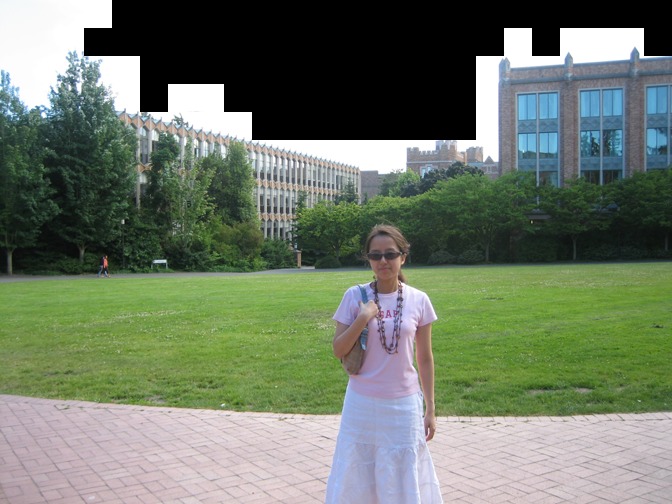
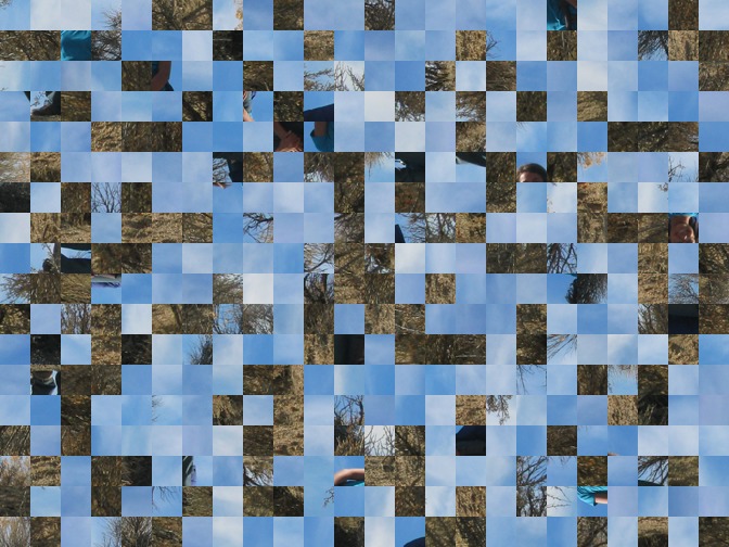
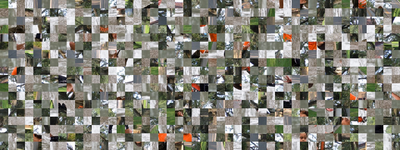
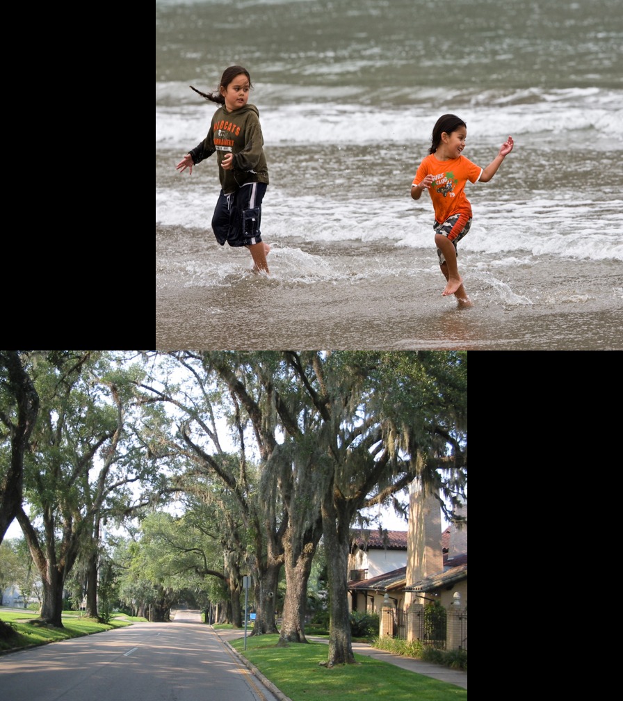
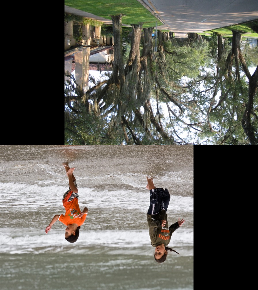
Mixed Type 2 Puzzles: Figure 5 shows the mixed puzzle reconstruction result of our approach. The input are the $864$ scrambled pieces ($432$ pieces per image) taken from two images of MIT dataset. It can be seen that our method successfully recovers all the $4$ rotation versions of the two images.

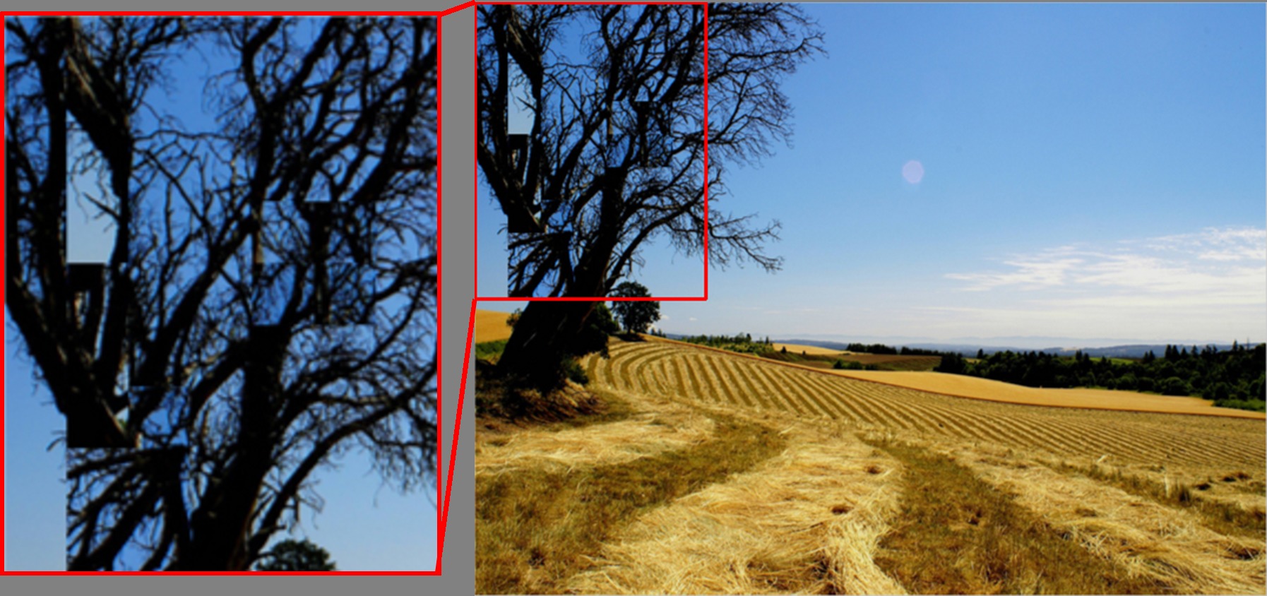
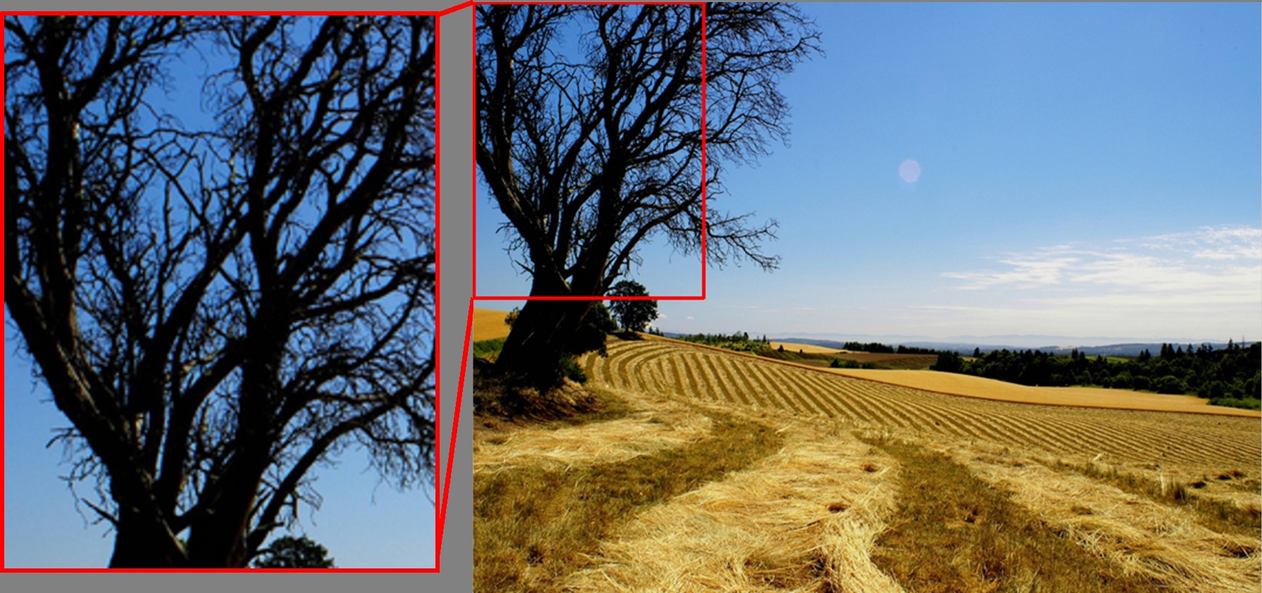
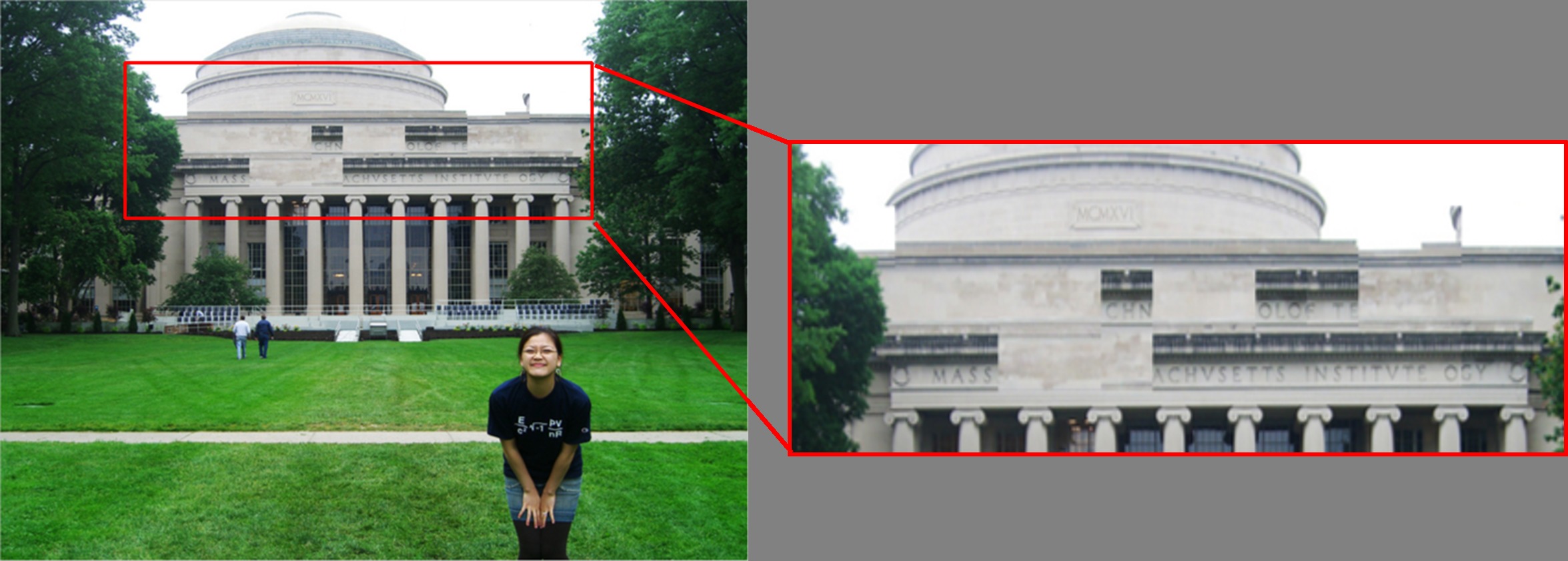
Experiment with noise: To further illustrate the robustness of our method, we conduct experiments with image noise on Type 2 puzzles from MIT dataset. Figure 7 shows the comparison of our approach with Gallagher [8] and Son et al. [16] at different levels of image noise, where we show a large gap in performance of our LP-based puzzle solver. This further illustrates its clear dominance with respect to competing approaches in the presence of noise.

Runtime: Our approach takes $5$ seconds for a $432$ piece Type 1 puzzle and $1$ minute for a Type 2 puzzle on a modern PC. The principal bottle-neck of the algorithm remains Gallagher’s $O(n^{2})$ computation of pairwise matches which is common to all state-of-the-art approaches[8, 16]. As such over the scale of problems considered, the algorithm complexity scales roughly quadratically with the number of the pieces of the puzzle.

5 Conclusion

We have proposed a novel formulation for solving jigsaw puzzles as a convergent sequence of linear programs. The solutions to these programs correspond to a sequence of unambiguous matches that have been proved to be globally consistent. Without any significant increase in runtime our approach outperforms existing global [14, 4, 19, 2] and greedy methods [8, 16] which represent state-of-the-art performance. Our system would extend naturally beyond 2D jigsaws to the reconstruction of damaged 3d objects[10] and mosaics[9] and this remains an exciting direction for future research.

References

- [1] T. Altman. Solving the jigsaw puzzle problem in linear time. Applied Artificial Intelligence an International Journal, 3(4):453–462, 1989.
- [2] F. A. Andaló, G. Taubin, and S. Goldenstein. Solving image puzzles with a simple quadratic programming formulation. In Graphics, Patterns and Images (SIBGRAPI), 2012 25th SIBGRAPI Conference on, pages 63–70. IEEE, 2012.
- [3] D. Ceylan, N. J. Mitra, Y. Zheng, and M. Pauly. Coupled structure-from-motion and 3d symmetry detection for urban facades. ACM Transactions on Graphics, 2013.
- [4] T. S. Cho, S. Avidan, and W. T. Freeman. A probabilistic image jigsaw puzzle solver. In Computer Vision and Pattern Recognition (CVPR), 2010 IEEE Conference on, pages 183–190. IEEE, 2010.
- [5] M. Cummins and P. Newman. Probabilistic appearance based navigation and loop closing. In Proc. IEEE International Conference on Robotics and Automation (ICRA’07), Rome, April 2007.
- [6] E. D. Demaine and M. L. Demaine. Jigsaw puzzles, edge matching, and polyomino packing: Connections and complexity. Graphs and Combinatorics, 23(1):195–208, 2007.
- [7] H. Freeman and L. Garder. Apictorial jigsaw puzzles: The computer solution of a problem in pattern recognition. Electronic Computers, IEEE Transactions on, (2):118–127, 1964.
- [8] A. C. Gallagher. Jigsaw puzzles with pieces of unknown orientation. In CVPR 2012, 2012.
- [9] A. García Castañeda, B. Brown, S. Rusinkiewicz, T. Funkhouser, and T. Weyrich. Global consistency in the automatic assembly of fragmented artefacts. In Proc. of 12th International Symposium on Virtual Reality, Archaeology and Cultural Heritage (VAST), pages 313–330, October 2011.
- [10] Q.-X. Huang, S. Flöry, N. Gelfand, M. Hofer, and H. Pottmann. Reassembling fractured objects by geometric matching. In ACM SIGGRAPH 2006 Papers, SIGGRAPH ’06, 2006.
- [11] D. A. Kosiba, P. M. Devaux, S. Balasubramanian, T. L. Gandhi, and R. Kasturi. An automatic jigsaw puzzle solver. In Pattern Recognition, 1994. Vol. 1-Conference A: Computer Vision & Image Processing., Proceedings of the 12th IAPR International Conference on, volume 1, pages 616–618. IEEE, 1994.
- [12] A. Olmos et al. A biologically inspired algorithm for the recovery of shading and reflectance images. Perception, 33(12):1463–1473, 2003.
- [13] D. Pomeranz, M. Shemesh, and O. Ben-Shahar. A fully automated greedy square jigsaw puzzle solver. In Computer Vision and Pattern Recognition (CVPR), 2011 IEEE Conference on, pages 9–16. IEEE, 2011.
- [14] D. Sholomon, O. David, and N. S. Netanyahu. A genetic algorithm-based solver for very large jigsaw puzzles. In Computer Vision and Pattern Recognition (CVPR), 2013 IEEE Conference on, pages 1767–1774. IEEE, 2013.
- [15] D. Sholomon, O. E. David, and N. S. Netanyahu. A generalized genetic algorithm-based solver for very large jigsaw puzzles of complex types. In Twenty-Eighth AAAI Conference on Artificial Intelligence, 2014.
- [16] K. Son, J. Hays, and D. Cooper. Solving square jigsaw puzzles with loop constraints. In ECCV 2014, 2014.
- [17] R. W. Webster, P. S. LaFollette, and R. L. Stafford. Isthmus critical points for solving jigsaw puzzles in computer vision. Systems, Man and Cybernetics, IEEE Transactions on, 21(5):1271–1278, 1991.
- [18] H. Wolfson, E. Schonberg, A. Kalvin, and Y. Lamdan. Solving jigsaw puzzles by computer. Annals of Operations Research, 12(1):51–64, 1988.
- [19] X. Yang, N. Adluru, and L. J. Latecki. Particle filter with state permutations for solving image jigsaw puzzles. In Computer Vision and Pattern Recognition (CVPR), 2011 IEEE Conference on, pages 2873–2880. IEEE, 2011.