Transductive Zero-Shot Action Recognition by Word-Vector Embedding

Abstract

The number of categories for action recognition is growing rapidly and it has become increasingly hard to label sufficient training data for learning conventional models for all categories. Instead of collecting ever more data and labelling them exhaustively for all categories, an attractive alternative approach is “zero-shot learning” (ZSL). To that end, in this study we construct a mapping between visual features and a semantic descriptor of each action category, allowing new categories to be recognised in the absence of any visual training data. Existing ZSL studies focus primarily on still images, and attribute-based semantic representations. In this work, we explore word-vectors as the shared semantic space to embed videos and category labels for ZSL action recognition. This is a more challenging problem than existing ZSL of still images and/or attributes, because the mapping between video space-time features of actions and the semantic space is more complex and harder to learn for the purpose of generalising over any cross-category domain shift. To solve this generalisation problem in ZSL action recognition, we investigate a series of synergistic strategies to improve upon the standard ZSL pipeline. Most of these strategies are transductive in nature which means access to testing data in the training phase. First, we enhance significantly the semantic space mapping by proposing manifold-regularized regression and data augmentation strategies. Second, we evaluate two existing post processing strategies (transductive self-training and hubness correction), and show that they are complementary. We evaluate extensively our model on a wide range of human action datasets including HMDB51, UCF101, OlympicSports and event datasets including CCV and TRECVID MED 13. The results demonstrate that our approach achieves the state-of-the-art zero-shot action recognition performance with a simple and efficient pipeline, and without supervised annotation of attributes. Finally, we present in-depth analysis into why and when zero-shot works, including demonstrating the ability to predict cross-category transferability in advance.

1 Introduction

Action recognition is of established importance in the computer vision community due to its potential applications in video retrieval, surveillance and human machine interaction (Aggarwal and Ryoo, 2011). However the need for increasing coverage and finer classification of human actions means the number and complexity of action categories of interest for recognition is growing rapidly. For example, action recognition dataset size and number of categories has experienced constant growth since the classic KTH Dataset (Schuldt et al, 2004) (6 classes, 2004): Weizmann Dataset (Blank et al, 2005) (9 classes, 2005), Hollywood2 Dataset (Marszalek et al, 2009) (12 classes, 2009), Olympic Sports Dataset (Niebles, 2010) (16 classes, 2010), HMDB51 (Kuehne et al, 2011) (51 classes, 2011) and UCF101 (Soomro et al, 2012) (101 classes, 2012). The growing number and complexity of actions result in: (1) Enormous human effort is required to collect and label large quantities of video data for learning. Moreover, compared to image annotation, obtaining each annotated action clip is more costly as it typically requires some level of spatio-temporal segmentation from the annotator. (2) The growing number of categories eventually begins to pose ontological difficulty, about how to structure and define distinct action categories as they grow more fine-grained and inter-related (Jiang et al, 2015). In this work, we explore methods which do not explicitly create models for new action categories from manually annotated training data, but rather dynamically construct recognition models by combining past experience in language together with knowledge transferred from already labelled existing action categories.

The “zero-shot learning” (ZSL) paradigm (Lampert et al, 2009; Fu et al, 2012; Socher et al, 2013) addresses this goal by sharing information across categories; and crucially by allowing recognisers for novel/ unseen/ testing categories to be constructed based on a semantic description of the category, without any labelled visual training samples. ZSL methods follow the template of learning a general mapping between a visual feature and semantic descriptor space from known/ seen/ training data . In the context of zero-shot action recognition, ‘semantic descriptor’ refers to an action class description that can be specified by a human user, either manually, or with reference to existing knowledge bases, e.g. wikipedia. The ZSL paradigm is most commonly realised by using class-attribute descriptors (Lampert et al, 2014; Liu et al, 2011; Fu et al, 2015a) to bridge the semantic gap between low-level features (e.g. MBH or SIFT) and categories. Attributes are mid-level concepts that transcend class boundaries (Lampert et al, 2009), allowing each category or instance to be represented as a binary (Lampert et al, 2009; Liu et al, 2011) or continuous (Fu et al, 2014b) vector. Visual attribute classifiers are learned for a set of known categories, and then a human can create recognisers for novel categories by specifying their attributes. With a few exceptions (Liu et al, 2011; Fu et al, 2015a; Xu et al, 2015), this paradigm has been applied to images rather than video action recognition.

An emerging alternative to attribute-based ZSL is unsupervised semantic embeddings (Socher et al, 2013; Frome et al, 2013; Fu et al, 2014b; Habibian et al, 2014b; Norouzi et al, 2014; Fu et al, 2015b; Xu et al, 2015; Akata et al, 2015).Unsupervised semantic embedding spaces refer to intermediate representations which can be automatically constructed from existing unstructured knowledge-bases (such as wikipedia text), rather than manually specified attributes. The most common approaches (Socher et al, 2013; Fu et al, 2014b, 2015b; Xu et al, 2015; Akata et al, 2015) are to exploit a distributed vector representation of words produced by a neural network (Mikolov et al, 2013) trained on a large text corpus in an unsupervised manner. Regressors (cf classifiers in the attribute space), are trained on the known dataset to map low-level visual features into this semantic embedding space. Zero-shot recognition is subsequently performed by mapping novel category visual instances to the embedding space via the regression, and matching these to the vector representation of novel class names (e.g. by nearest neighbour). Several properties make the embedding space approaches preferable to the attribute-based ones: (1) A manually pre-defined attribute ontology is not needed as embedding space is learned in an unsupervised manner. (2) Novel categories can be defined trivially by naming them, without the requirement to exhaustively define each class in terms of a list of attributes – which grows non-scale-ably as the breadth of classes to recognise grows (Fu et al, 2014b; Akata et al, 2015). (3) Semantic embedding allows easier exploitation of information sharing across datasets (Xu et al, 2015; Habibian et al, 2014b) because category names from multiple datasets can be easily projected into a common embedding space, while attribute spaces are usually dataset specific, with datasets having incompatible attribute schemas (e.g. UCF101 (Jiang et al, 2013) and Olympic Sports (Liu et al, 2011) have disjoint attribute sets).

The domain shift problem for ZSL of actions Although embedding-based ZSL is an attractive paradigm, it has rarely previously been demonstrated in zero-shot action recognition. This is in part because of the pervasive challenge of learning mappings, that generalize across the train-test semantic gap (Fu et al, 2015a; Romera-Paredes and Torr, 2015). In ZSL, the train-test gap is more significant than conventional supervised learning because the training and testing classes are disjoint, i.e. completely different without any overlap. As a result of serious domain-shift (Pan and Yang, 2010), mapping from low-level visual feature to semantic embedding trained on a known class data will generalise poorly to novel class data. This is because the data distributions for the underlying categories are different. This violates the assumptions of supervised learning methods and results in poor performance. The domain shift problem – analysed empirically in Fu et al (2015a); Dinu et al (2015), and theoretically in Romera-Paredes and Torr (2015) – is worse for action than still image recognition because of the greater complexity of categories in visual space-time features and the mapping of space-time features to semantic embedding space.

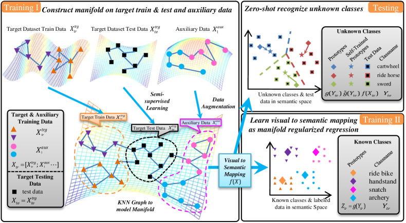
Our Solutions In this work, we explore four potential solutions to ameliorate the domain shift challenge in ZSL for action recognition as shown in Fig. 1, and achieve better zero-shot action recognition: (1) The first strategy we consider aims to improve the generalisation of the embedding space mapping. We explore manifold regularization (aka semi-supervised learning) to learn a regressor which exploits a regularizer based on the testing/unlabelled data to learn a smoother regressor that better generalises to novel testing classes. Manifold regularization (Belkin et al, 2006) is established in semi-supervised learning to improve generalisation of predictions on testing data, but this is more important in ZSL since the gap between training and testing data is even bigger due to disjoint categories. To our best knowledge, this is the first transductive use of testing/unlabelled data for zero-shot learning at training time. (2) The second strategy we consider is data augmentation (aka cross-dataset transfer learning) (Pan and Yang, 2010; Shao et al, 2015). The idea is that by simultaneously learning the regressors for multiple action datasets, a more representative sample of input action data is seen, and thus a more generalizable mapping from the visual feature to the semantic embedding space is learned. This is straightforward to achieve with semantic embedding-based ZSL because the datasets and their category name word-vectors can be directly aggregated. In contrast, it is non-trivial with attribute-based ZSL due to the need to develop a universal attribute ontology for all datasets. Besides these two new considerations to expand the embedding projection, we also evaluate two existing post-processing heuristics to reduce the effect of domain-shift in ZSL. These include (3) self-training, which adapts test-class descriptors based on unlabeled testing data to bridge the domain shift (Fu et al, 2014c) and (4) Hubness correction which re-ranks the test-data’s match to novel class descriptions in order to avoid the bias toward ‘hub’ categories induced by domain shift (Dinu et al, 2015).

By exploring manifold regularization, data augmentation, self-training, and hubness correction, our word-vector embedding approach outperforms consistently conventional zero-shot approaches on all contemporary action datasets (HMDB51, UCF101, Olympic Sports, CCV and USAA). On a more relaxed multi-shot setting, our representation is comparable with using low-level features directly. Interestingly, with unsupervised semantic embedding (word-vector) and transductive access to testing data we are able to achieve very competitive performance even compared to supervised embedding methods (Fu et al, 2014b; Akata et al, 2015) which require attribute annotation. Moreover, because our method has a closed-form solution to the visual to semantic space mapping, it is very simple to implement, requiring only a few lines of Matlab.

Transductive Setting Of the four strategies, manifold regularization, self-training, and hubness correction assume access to the full set of unlabelled testing data, which is called the transductive setting (Belkin et al, 2006; Fu et al, 2015a). This assumption would be true in many real-world problems. Video repositories, e.g. YouTube, can process large batches of unlabelled videos uploaded by users. Transductive zero-shot methods can be used to tag batches automatically without manual annotation, or add a new tag to the ontology of an existing annotated set.

New Insights In order to better understand ZSL, this study performs a detailed analysis of the relationship between training and testing classes for zero-shot learning, revealing the causal connection between known and novel category recognition performance.

Contributions Our key contributions are threefold: (1) We explore jointly four mechanisms for expanding ZSL by addressing its domain-shift challenge, including three transductive learning strategies - manifold regularization, self-training and hubness correction. Our model is both closed-form in solving the visual to semantic mapping and unsupervised in constructing the semantic embeddings. (2) We show extensive experiments to demonstrate a very simple implementation of this closed-form model that both runs very quickly and is capable of achieving the state-of-the-art ZSL performance on contemporary action/event datasets. (3) We provide new insight, for the first time, into the underlying factors affecting the efficacy of ZSL.

Figure 1: We have labelled data in target dataset $\mathbf{X}^{trg}_{tr}$ and auxiliary dataset $\mathbf{X}^{aux}_{1}$ and testing data in target dataset $\mathbf{X}^{trg}_{te}$. The objective is to use all this data to classify testing data into a set of pre-defined categories (aka unknown classes). Specifically, in the training phase I, target labelled data $\mathbf{X}^{trg}_{tr}$ is first augmented by data from auxiliary dataset $\mathbf{X}^{aux}_{1}$ to form a combined labelled dataset $\mathbf{X}_{tr}$. We construct a K Nearest Neighbour (KNN) graph on all labelled and testing data in visual feature space to model the underlying manifold structure. In the training phase II, prototypes for known classes are generated by semantic embedding $\mathbf{Z}_{tr}=g(\mathbf{y}_{tr})$. Then we learn a visual-to-semantic mapping $f:\mathbf{X}_{tr}\to\mathbf{Z}_{tr}$ as manifold regularized regression. In the testing phase, prototypes for unknown classes are first generated by semantic embedding $g(\mathbf{y}_{te})$. Then target testing data $\mathbf{X}_{te}$ are projected into semantic space via $f(\mathbf{X})$. Finally simple nearest neighbour (NN) classifier is used to categorize testing data as the label of closest prototype. On top of NN classifier, self-training and hubness corrections are adopted at testing phase to improve results by mitigating the domain shift problem. With this framework we achieve the state-of-the-art performance on zero-shot action recognition tasks.

2 Related Work

2.1 Action Recognition

Video action recognition is now a vast and established area in computer vision and pattern recognition due to the wide application in video surveillance, interaction between human and electronic devices. Extensive surveys of this area are conducted by Aggarwal and Ryoo (2011); Poppe (2010). Recent progress in this area is attributed to densely tracking points and computing hand-crafted features which are fed into classical supervised classifiers (e.g. SVM) for recognition (Wang et al, 2015).

Human Action Datasets Video datasets for action recognition analysis have experienced constant developing. Early datasets focus on simple and isolated human actions performed by a single person, e.g. KTH (Schuldt et al, 2004) (2004) and Weizmann (Blank et al, 2005) (2005) datasets. Due to the growth of internet video sharing, e.g. YouTube and Vimeo, action datasets collected from online repositories are emerging, e.g. OlympicSports (Niebles, 2010) in 2010, HMDB51 (Kuehne et al, 2011) in 2011 and UCF101 (Soomro et al, 2012) in 2012.

Event Datasets To recognize more complex events with interactions between people and objects, event datasets including Columbia Consumer Video dataset (CCV) (Jiang et al, 2011) and the TRECVID Multimedia Event Detection (MED) dataset (Over et al, 2014) are becoming popular.

Feature Representation Local space-time feature approaches have become the the prevailing strategies due to not requiring non-trivial object tacking and segmentation. In these approaches, local interest points are first detected (Laptev, 2005) or densely sampled (Wang et al, 2015). Visual descriptors invariant to clutter, appearance and scale are calculated in a spatiotemporal volume formed by the interest points. Different visual descriptors have been proposed to capture the texture, shape and motion information, including 3D-SIFT (Scovanner et al, 2007), HOG3D (Klaser et al, 2008) and local trinary patterns (Yeffet and Wolf, 2009). Among these, dense trajectory features with HOG, HOF and MBH descriptors (Wang et al, 2013) and its variant improved trajectory features (Wang et al, 2015) produce state-of-the-art performance on action recognition. Therefore, we choose improved trajectory feature (ITF) for our low-level feature representation.

2.2 Zero-Shot Learning

Zero-shot learning aims to achieve dynamic construction of classifiers for novel classes at testing time based on semantic descriptors provided by humans or existing knowledge bases, rather than labeled examples. This approach was popularised by the early studies (Larochelle et al, 2008; Palatucci et al, 2009; Lampert et al, 2009). Since then numerous studies have been motivated to investigate ZSL due to the scalability barrier of exhaustive annotation for supervised learning, and the desire to emulate the human ability to learn from description with few or no examples.

ZSL Architectures Various architectures have been proposed for zero-shot recognition of classes $\mathbf{y}$ given data $\mathbf{X}$. Sequential architectures (Lampert et al, 2009; Fu et al, 2014b, 2015a; Liu et al, 2011; Zhao et al, 2013; Lazaridou et al, 2014; Norouzi et al, 2014) setup classifier/regressor mappings $\mathbf{Z}=f(\mathbf{X})$ to predict semantic representations $\mathbf{Z}$, followed by a recognition function $\mathbf{y}=r(\mathbf{Z})$. The visual feature mapping $f(\cdot)$ is learned from training data and assumed to generalise, and the recogniser is given by the human or external knowledge. Converging architectures (Akata et al, 2015; Yang and Hospedales, 2015; Romera-Paredes and Torr, 2015; Frome et al, 2013) setup energy functions $E(\mathbf{X},\mathbf{Z})$ which are positive when $\mathbf{X}$ and $\mathbf{Z}$ are from matching classes and negative otherwise. In this work, we adopt a sequential regression approach for simplicity and efficiency of closed-form solution, and amenability to exploiting the unlabelled data manifold.

Attribute Embeddings The most popular intermediate representation for ZSL has been attributes, where categories are specified in terms of a vector of binary (Lampert et al, 2009; Liu et al, 2011; Zhao et al, 2013) or continuous (Fu et al, 2014b; Akata et al, 2015; Romera-Paredes and Torr, 2015) attributes. However, this approach suffers inherently from the need to agree upon a universal attribute ontology, and the scalability barrier of manually defining each new class in terms of an attribute ontology that grows with breadth of classes considered (Fu et al, 2014b; Akata et al, 2015).

Word-Vector Embeddings While other representations including taxonomic (Akata et al, 2015), co-occurence (Gan et al, 2015; Mensink et al, 2014; Habibian et al, 2014b) and template-based (Larochelle et al, 2008) have been considered, word-vector space ZSL (Fu et al, 2015a; Akata et al, 2015; Xu et al, 2015; Lazaridou et al, 2014; Norouzi et al, 2014; Frome et al, 2013) has emerged as the most effective unsupervised alternative to attributes. In this approach, the semantic class descriptor $\mathbf{Z}$ is generated automatically from existing unstructured text knowledge bases such as the Wikipedia. In practice, this often means the target $\mathbf{Z}$ of mapping $\mathbf{Z}=f(\mathbf{X})$ is given by the internal representation of a text modelling neural network (Mikolov et al, 2013). This can be more intuitively understood as encoding each class name in terms of a vector describing its co-occurance frequency with other terms in a text corpus (Lazaridou et al, 2014). In sequential architectures the final recognition is typically performed with nearest neighbour (NN) matching of the predicted class descriptor (Xu et al, 2015; Lazaridou et al, 2014; Norouzi et al, 2014).

Domain-Shift Every ZSL method suffers from the issue of domain shift between the training class on which the mapping $f(\cdot)$ or energy function $E(\cdot,\cdot)$ is trained, and the disjoint set of testing classes to which it is tested on. Although this is a major reason why it is hard to obtain competitive results with ZSL strategies, it is only recently this problem has been studied explicitly (Dinu et al, 2015; Fu et al, 2015a; Romera-Paredes and Torr, 2015). In this work, we focus primarily on how to mitigate this domain-shift problem in ZSL for action recognition. That is, by making the training data more representative thus learning a more general visual feature to semantic space mapping (dataset augmentation), transductively exploiting both labelled and unlabelled data manifold to learn an embedding mapping that generalises better to the testing data (manifold regularized regression), and post-processing corrections to adapt (self-training) the classifier at the testing time therefore to improve its robustness (hubness correction) to domain shift. While transductive (Dinu et al, 2015; Fu et al, 2015a; Xu et al, 2015) strategies have been exploited before as post-processing, this is the first time it have been exploited for learning the embedding itself via manifold regression.

ZSL Insights Previous studies have provided particular insight into the ZSL problem, including Rohrbach et al (2010); Akata et al (2015) who focus on exploring and comparing different class-label embeddings (we use word-vectors), Rohrbach et al (2011) who explores scalability to large scale settings, and Dinu et al (2015) who discusses why ZSL is harder than supervised learning due to the hubness problem. Our insights aim to complement the above studies by exploring when positive transfer occurs, and showing how it is possible to predict this in advance.

2.3 ZSL for Action Recognition

Despite clear appeal from ZSL, few studies have considered it for action recognition. Early attribute-centric studies took latent SVM (Liu et al, 2011) and topic model (Fu et al, 2014b; Zhao et al, 2013) approaches, neither of which are very scalable for large video datasets. Thus more recent studies have started to consider unsupervised embeddings including semantic relatedness (Gan et al, 2015) and word-vectors (Xu et al, 2015). However, most prior ZSL action recognition studies do not evaluate against a wide range of realistic set of contemporary action recognition benchmarks, restricting themselves to a single dataset of USAA (Fu et al, 2014b; Zhao et al, 2013), or Olympic Sports (Liu et al, 2011). In this work, we fully explore word-vector-based zero-shot action recognition, and demonstrate its superiority to attribute-based approaches, despite the latter’s supervised ontology construction. Another line of work towards zero-shot action recognition have been studied by Jain et al (2015) who proposed to exploit the vast object annotations, images and textual descriptions, e.g. ImageNet (Deng et al, 2009).

2.4 ZSL for Event Detection

In contrast to action recognition, another line of work on the related task of event detection typically deals with temporally longer multimedia videos. The most widely studied test is the TRECVID Multimedia Event Detection (MED) benchmark (Over et al, 2014). In the zero-shot MED task (MED 0EK), 20 events are to be detected among a 27K video (Test Set MED) with no positive examples of each test event available for training. Existing studies (Wu et al, 2014; Chen et al, 2014; Habibian et al, 2014a) typically discover a ‘concept space’ by extracting frequent terms with pruning in video metadata (per-video text description) and learning concept classifiers on the 10K video Research Set. Then for each of the 20 events to be detected, a query is generated as a concept vector from the metadata of the event (textual description of event) (Wu et al, 2014) or an event classifier is learned on 10 positive examples of the testing event (Habibian et al, 2014a). The testing videos are finally tested against the concept classifiers and then matched to the query as inner product between concept detection scores and query concepts (Wu et al, 2014) or through the event classifier (Habibian et al, 2014a). Alternatively, visual concept can be mined from noisy online image repositories. In the concept space, a query is then generated from event name and keywords which are extracted from event definitions (Chen et al, 2014). These approaches rely on two assumptions: (1) A large concept training pool (10K video) with per-video textual description annotated by experts. (2) A detailed description of the event to be detected is needed to generate the query. For example a typical event description includes the name - ‘Birthday Party’, Explication - ‘A birthday in this context is the anniversary of a person’s birth etc’, Object/People - ‘Decorations, birthday cake, candles, gifts, etc’. Since detailed per-video annotations and detailed descriptions of event types are not widely available in other video databases, in this work we focus on exploring the TRECVID task with the more challenging but also more broadly applicable setting of event name-driven training and queries only. This setting is rarely studied for TRECVID, except in the recent study (Jain et al, 2015) which explores using a Fisher vector to encode compound event/action names.

3 Methodology

To formalise the problem a list of notations are first given in Table 1. We have a training video set $\mathbf{T}_{tr}=\{\mathbf{X}_{tr},\mathbf{y}_{tr}\}$ where $\mathbf{X}_{tr}=\{\mathbf{x}_{i}\}_{i=1\cdots n_{l}}$ is the set of $d_{x}$ dimensional low-level features, e.g. Fisher Vector encoded MBH and HOG. For each of the $n_{l}$ labelled training videos $\mathit{y}_{i}$ is the class names/labels of each instance, e.g. “brush hair” and “handwalk”. We also have a set of testing videos $\mathbf{T}_{te}=\{\mathbf{X}_{te},\mathbf{y}_{te}\}$ with $n_{u}$ unlabelled testing video instances. The goal of ZSL is to learn to recognise videos in $\mathbf{X}_{te}$ whose classes $\mathbf{y}_{te}$ are disjoint from any seen data at training time: $\mathbf{y}_{tr}\cap\mathbf{y}_{te}=\emptyset$.

Table 1: Basic notations.

Notation	Description
$\mathbf{X}\in\mathbb{R}^{d_{x}\times N}$; $\mathbf{x}_{i}$	Visual feature matrix for N instances; Column representing the $i$-th instance
$\mathbf{y}\in\mathbb{Z}^{1\times N}$; $\mathit{y}_{i}$	Integer class labels for N instances; Scalar representing the $i$-th instance
$\mathbf{Z}\in\mathbb{R}^{d_{z}\times N}$; $\mathbf{z}_{i}$	Semantic embedding for N instances; Column representing the $i$-th instance
$\mathbf{K}\in\mathbb{R}^{N\times N}$	Kernel matrix
$\mathbf{A}\in\mathbb{R}^{d_{z}\times N}$	Regression coefficient matrix
$f:\mathbf{X}\to\mathbf{Z}$	Visual to semantic mapping function
$g:\mathbf{y}\to\mathbf{Z}$	Class name embedding function
$\lambda_{A}\in\mathbb{R}$	Ridge regression regularizor
$\lambda_{I}\in\mathbb{R}$	Manifold regression regularizor
$N^{G}_{K}\in\mathbb{Z}^{+}$	KNN Graph parameter for manifold regularizor
$N^{st}_{K}\in\mathbb{Z}^{+}$	KNN parameter for Self-Training procedure

3.1 Semantic Embedding Space

To bridge the gap between disjoint training and testing classes, we establish a semantic embedding space $\mathbf{Z}$ based on word-vectors. In particular we use a neural network (Mikolov et al, 2013) trained on a 100 billion word corpus to realise a mapping $g:\mathbf{y}\to\mathbf{Z}$ that produces a unique $d_{z}$ dimensional encoding vector of each dictionary word.

Compound Names The above procedure only deals with class names that are unigram dictionary words. To process compound names commonly occurring in action datasets, e.g. “brush hair” or “ride horse”, that do not exist as individual tokens in the corpus, we exploit compositionally of the semantic space (Mitchell and Lapata, 2008). Various composition methods have been proposed (Mitchell and Lapata, 2008; Milajevs et al, 2014) including additive, multiplicative and others, but our experiments showed no significant to using others besides addition, so we stick with simple additive composition.

Suppose the $ith$ class name $\mathit{y}_{i}$ is composed of words $\{y_{ij}\}_{j=1\cdots w}$. We generate a single $d_{z}$ dimensional vector $\mathbf{z}$ out of the word-vector $\mathit{y}_{i}$ by a averaging word-vectors for constituent words $\{y_{ij}\}$:

$$\mathbf{z}_{i}=\frac{1}{w}\cdot\sum_{j=1}^{w}g(y_{ij})$$ (1)

3.2 Visual to Semantic Mapping

Mapping by Regression: In order to map video features into the semantic embedding space constructed above, we train a regression model $f:X\to Z$ from $d_{x}$ dimensional low-level visual feature space to the $d_{z}$ dimensional embedding space. The regression is trained using training instances $\mathbf{X}_{tr}=\{\mathbf{x}_{i}\}_{i=1\cdots n_{l}}$ and the corresponding embedding $\mathbf{Z}_{tr}=g(\mathbf{y}_{tr})$ of the instance class name $\mathit{y}$ as the target value. Various methods have previously been used for this task including linear support vector regression (SVR) (Fu et al, 2014b, 2015a; Xu et al, 2015) and more complex multi-layer neural networks (Socher et al, 2013; Lazaridou et al, 2014; Yang and Hospedales, 2015). Since we will use fisher vector encoding (Perronnin et al, 2010) for features $\mathbf{X}$, we can easily apply simple linear regression for $f(\cdot)$. Specifically, we use $l_{2}$ regularized linear regression (aka ridge regression) to learn the visual to semantic mapping.

Kernel Ridge Regression: The fisher vector encoding generates a very high dimensional feature $2\times d_{descr}\times N_{k}$ where $N_{k}$ is the number of components in the Gaussian Mixture Model (GMM) and $d_{descr}$ is the dimension of raw descriptors. This usually results in many more feature dimensions than training samples. Thus we use the representer theorem (Scholkopf and Smola, 2002) and formulate a kernelized ridge regression with a linear kernel in Eq (2). The benefit of kernelised regression is to reduce computation as the closed-form solution to $\mathbf{A}$ only involves computing the inverse of a $N\times N$ rather than a $d_{x}\times d_{x}$ matrix where $N<d_{x}$.

$$\mathit{k}(x_{i},x_{j})=\sum\limits_{d=1}^{d_{x}}(x_{id}\cdot x_{jd})$$ (2)

The visual features $\mathbf{x}$ can be then projected into semantic space via Eq (3) where $\mathbf{a}_{j}$ is the $j$th column of regression parameter matrix $\mathbf{A}$.

$$f(\mathbf{x})=\sum\limits_{j=1}^{n_{l}}\mathbf{a}_{j}\mathit{k}(\mathbf{x},\mathbf{x}_{j})$$ (3)

To improve the generalisation of the regressor, we add the $l_{2}$ regularizer $||f||_{\mathbf{K}}^{2}=Tr(\mathbf{A}\mathbf{K}\mathbf{A}^{T})$ to reduce overfitting by penalising extreme values in the regression matrix. This gives the kernel ridge regression loss:

$$\begin{split}&\min_{f}\frac{1}{n_{l}}\sum\limits_{i=1}^{n_{l}}||\mathbf{z}_{i}-f(\mathbf{x}_{i})||^{2}_{2}+\gamma||f||^{2}_{K}\\ &\min_{\mathbf{A}}\frac{1}{n_{l}}Tr\left((\mathbf{Z}-\mathbf{AK})^{T}(\mathbf{Z}-\mathbf{AK})\right)+\gamma Tr(\mathbf{AKA}^{T})\end{split}$$ (4)

where the regression targets are generated by the vector representation of each class name $\mathbf{z}_{i}=g(\mathit{y}_{i})$ and $\mathbf{Z}=[\mathbf{z}_{1}\>\mathbf{z}_{2}\cdots]_{d_{z}\times n_{l}}$, $\mathbf{A}$ is the $d_{z}\times n_{l}$ regression coefficient matrix, $\mathbf{K}$ is the $n_{l}\times n_{l}$ kernel matrix and $n_{l}$ is the number of labelled training instances. The loss function is convex with respect to the $\mathbf{A}$. Taking derivatives w.r.t $\mathbf{A}$ and setting the gradient to 0 leads to the following closed-form solution where $\mathbf{I}$ is the identity matrix.

$$\mathbf{A}={\mathbf{Z}}\left(\mathbf{K}+\gamma_{A}n_{l}\mathbf{I}\right)^{-1}$$ (5)

The above mapping by Kernel Ridge Regression provides a simple solution to embed visual instances into semantic space. However the simple ridge regression only considers limited labelled training data $\mathbf{X}_{tr}$ without exploiting the underline structure of the manifold on both labelled and unlabelled data nor any additional related labelled data from other datasets. In the following sections, we introduce two approaches to improve the quality of mapping: (1) Manifold-Regularized Regression and (2) Data Augmentation.

3.2.1 Manifold Regularized Regression

As discussed earlier, conventional regularization provides poor ZSL due to disjoint training and testing classes. To improve recognition of testing classes, we explore transductive semi-supervised regression. The idea is to exploit unlabelled testing data $\mathbf{X}_{te}$ to discover the manifold structure in the zero-shot classes, and preserve this structure in the semantic space after visual-semantic mapping. Therefore, this is also known as manifold regularization. Note that we use labelled to refer to training data $\mathbf{X}_{tr}$ and unlabelled to refer to testing data $\mathbf{X}_{te}$. So we use semi-supervised manifold regularization in a transductive way, requiring access to the unlabelled/testing data $\mathbf{X}_{te}$ during the training phase.

To that end, we introduce manifold laplacian regularization (Belkin et al, 2006) into the ridge regression formulation. This additional regularization term ensures that if two videos are close to each other in the visual feature space, this relationship should be kept in the semantic space as well.

We model the manifold by constructing a symmetric K nearest neighbour (KNN) graph $\mathbf{W}$ on the all $n_{l}+n_{u}$ instances where $n_{l}=|\mathbf{T}_{tr}|$ denotes the number of labelled training instances and $n_{u}=|\mathbf{T}_{te}|$ denotes the number of unlabelled testing instances. The KNN Graph is constructed by first computing a linear kernel matrix between all instances. Then for each instance we select the top K neighbours and assign an edge between these nodes. This gives us a directed graph which is then symmetrized by converting to an undirected graph by connecting nodes with any directed edge between them. Let $\mathbf{D}$ be a diagonal matrix with $d_{ii}=\sum_{j=1}^{n_{l}+n_{u}}w_{ij}$, we get the graph laplacian matrix $\mathbf{L}=\mathbf{D}-\mathbf{W}$. The manifold regularizer is then written as:

Further denoting $\mathbf{f}=[f(\mathbf{x}_{1})\;f(\mathbf{x}_{2})\cdots\;f(x_{n_{l}+n_{u}})]=\mathbf{A}\mathbf{K}$. Eq. (6) can be rewritten in matrix form as:

$$\begin{split}||f||_{I}^{2}&=Tr(\mathbf{f}^{\top}\mathbf{f}\mathbf{D})-Tr(\mathbf{f}^{\top}\mathbf{f}\mathbf{W})\\ &=Tr(\mathbf{f}^{\top}\mathbf{f}\mathbf{L})\\ &=Tr(\mathbf{K}^{\top}\mathbf{A}^{\top}\mathbf{A}\mathbf{K}\mathbf{L})\end{split}$$ (7)

where $\mathbf{K}$ is a $(n_{l}+n_{u})\times(n_{l}\times n_{u})$ dimensional kernel matrix constructed upon all labelled and unlabelled instances via Eq (2). Combining all regularization terms we obtain the overall loss function in Eq (8), where for simplicity we denote $\mathbf{J}=\left[\begin{array}[]{ccc}\mathbf{I}_{n_{l}\times n_{l}}&\mathbf{0}_{n_{l}\times n_{u}}\\ \mathbf{0}_{n_{u}\times n_{l}}&\mathbf{0}_{n_{u}\times n_{u}}\end{array}\right]$ and $\tilde{\mathbf{Z}}=[\mathbf{Z}_{tr}\quad\mathbf{0}_{d_{z}\times n_{u}}]$. The final loss function can be thus written in the matrix form as:

The loss function is convex w.r.t. the $d_{z}\times(n_{l}+n_{u})$ regression coefficient matrix $\mathbf{A}$. A closed-form solution to $\mathbf{A}$ can be obtained in the same way as Kernel Ridge Regression.

$$\mathbf{A}=\tilde{\mathbf{Z}}\left(\mathbf{KJ}+\gamma_{A}n_{l}\mathbf{I}+\frac{\gamma_{I}n_{l}}{(n_{l}+n_{u})^{2}}\mathbf{KL}\right)^{-1}$$ (9)

Eq (9) provides an efficient way to learn the visual to semantic mapping due to the closed-form solution compared to alternative iterative approaches (Fu et al, 2014b; Habibian et al, 2014b). At testing time, the mapping can be efficiently applied to project new videos into the embedding with Eq. (3). Note when $\gamma_{I}=0$ manifold regression becomes exactly kernel regression.

3.2.2 Improving the Embedding with Data Augmentation

As discussed, the mapping often generalises poorly because: (i) actions are visually complex and ambiguous, and (ii) even a mapping well learned for training categories may not generalise well to testing categories as required by ZSL, because the volume of training data is small compared to the complexity of a general visual to semantic space mapping. The manifold regression described previously ameliorates the latter issues, but we next discuss a complementary strategy of data augmentation.

Another way to further mitigate both of these problems is by augmentation with any available auxiliary dataset which need not contain classes in common with the target testing dataset $\mathbf{T}^{trg}_{te}$in which zero-shot recognition is performed. This will provide more data to learn a better generalising regressor $\mathbf{z}=f(\mathbf{x})$. We formalize the data augmentation problem as follows. We denote the target dataset as $\mathbf{T}^{trg}=\{\mathbf{X}^{trg},\mathbf{y}^{trg}\}$ split into training set $\mathbf{T}^{trg}_{tr}=\{\mathbf{X}^{trg}_{tr},\mathbf{y}^{trg}_{tr}\}$ and zero-shot testing set $\mathbf{T}^{trg}_{te}=\{\mathbf{X}^{trg}_{te},\mathbf{y}^{trg}_{te}\}$. Zero-shot recognition is performed on the testing set of the target dataset (e.g. HMDB51). There are $n_{aux}$ other available auxiliary datasets $\mathbf{T}^{aux}_{i=1\cdots n_{aux}}=\{\mathbf{X}^{aux}_{i},\mathbf{y}^{aux}_{i}\}$ (e.g. UCF101, Olympic Sports and CCV). We propose to improve the regression by merging the target dataset training data and all auxiliary sets. The auxiliary dataset class names $\mathbf{y}^{aux}_{i}$ are projected into the embedding space with $\mathbf{Z}^{aux}_{i}=g(\mathbf{y}^{aux}_{i})$. The auxiliary instances $\mathbf{X}^{aux}$ are aggregated with the target training data as $\mathbf{X}_{tr}=[\mathbf{X}^{trg}_{tr}\;\mathbf{X}^{aux}_{1}\;\cdots\;\mathbf{X}^{aux}_{n_{aux}}]$ and $\mathbf{Z}_{tr}=[\mathbf{Z}^{trg}_{tr}\;\mathbf{Z}^{aux}_{1}\;\cdots\;\mathbf{Z}^{aux}_{n_{aux}}]$ where $\mathbf{Z}^{trg}_{tr}=g(\mathbf{y}^{trg}_{tr})$. The augmented training data $\mathbf{X}_{tr}$ and class embeddings $\mathbf{Z}_{tr}$ are used together to train the regressor $f$.

To formulate the loss function in matrix form we denote $n^{trg}_{l}=|\mathbf{T}^{trg}_{tr}|$, $n^{trg}_{u}=|\mathbf{T}^{trg}_{te}|$, $n^{aux}_{l}=\sum\limits_{i}|\mathbf{T}^{aux}_{i}|$. Let $\tilde{\mathbf{K}}$ be the $(n^{trg}_{tr}+n^{trg}_{te}+n^{aux}_{l})\times(n^{trg}_{tr}+n^{trg}_{te}+n^{aux}_{l})$ dimensional kernel matrix on all target and auxiliary data, and $\tilde{\mathbf{L}}$ is the corresponding graph laplacian. We then write the block structured $\tilde{\mathbf{J}}$ matrix as:

$$\tilde{\mathbf{J}}=\begin{bmatrix}\mathbf{I}_{(n_{l}^{trg}+n_{l}^{aux})\times(n_{l}^{trg}+n_{l}^{aux})}&\mathbf{0}\\ \mathbf{0}&\mathbf{0}_{n_{u}^{trg}\times n_{u}^{trg}}\end{bmatrix}$$ (10)

The loss function of manifold regularized regression with data augmentation is thus written in a matrix form as:

In the same way as before, we obtain the closed-form solution to $\mathbf{A}$:

where by setting $\gamma_{I}=0$ we obtain a kernel ridge regression with only data augmentation. This solution can be conveniently implemented in a single line of Matlab.

3.3 Zero-Shot Recognition

Given the trained mappings $f(\cdot)$ and $g(\cdot)$ we can now complete the zero-shot learning task. To classify a testing instance $\mathbf{x}^{*}\in\mathbf{X}_{te}$, we apply nearest neighbour matching of the projected testing instance $f(\mathbf{x}^{*})$ against the vector representations of all the testing classes $g(\mathit{y})$ (named the prototype throughout this paper):

$$\hat{\mathit{y}}=\arg\min_{\mathit{y}\in\mathbf{y}_{te}}\|f(\mathbf{x}^{*})-g(\mathit{y})\|$$ (13)

Distances in such embedding spaces have been shown to be best measured using the cosine metric (Mikolov et al, 2013; Fu et al, 2014b). Thus we $l_{2}$ normalise each data point, making Euclidean distance effectively equivalent to cosine distance in this space.

3.3.1 Ameliorating Domain Shift by Post Processing

In the previous two sections we introduced two methods to improve the embedding $f$ for ZSL. In this section we now discuss two post-processing strategies to further reduce the impact of domain shift.

Self-training for Domain Adaptation The domain shift induced by applying $f(\cdot)$ trained on $\mathbf{X}_{tr}$ to data of different statistics $\mathbf{X}_{te}$ means the projected data points $f(\mathbf{X}_{te})$ do not lie neatly around the corresponding class projections/prototypes $g(\mathbf{y}_{te})$ (Fu et al, 2015a). To ameliorate this domain shift, we explore transductive self-training to adjust unseen class prototypes to be more comparable to the projected data points. For each category prototype $g(\mathit{y}^{*}),\mathit{y}^{*}\in\mathbf{y}_{te}$ we search for the $N^{st}_{K}$ nearest neighbours among the unlabelled testing instance projections, and re-define the adapted prototype $\tilde{g}(\mathit{y}^{*})$ as the average of those $N^{st}_{K}$ neighbours. Thus if $NN_{K}(g(\mathit{y}^{*}))$ denotes the set of K nearest neighbours of $g(\mathit{y}^{*})$, we have:

$$\tilde{g}(\mathit{y}^{*}):=\frac{1}{N^{st}_{K}}\sum_{f(\mathbf{x}^{*})\in NN_{K}(g(\mathit{y}^{*}))}^{N^{st}_{K}}f(\mathbf{x}^{*})$$ (14)

The adapted prototypes $\tilde{g}(\mathit{y}^{*})$ are now more directly comparable with the testing data for matching using Eq. (13).

Hubness Correction One practical effect of the ZSL domain shift was elucidated in Dinu et al (2015), and denoted the ‘Hubness’ problem. Specifically, after the domain shift, there are a small set of ‘hub’ test-class prototypes that become nearest or K nearest neighbours to the majority of testing samples in the semantic space, while others are NNs of no testing instances. This results in poor accuracy and highly biased predictions with the majority of testing examples being assigned to a small minority of classes. We therefore explore the simple solutions proposed by Dinu et al (2015) which takes into account the global distribution of zero-shot samples and prototypes. This method is transductive as with self-training and manifold-regression. Specifically, we considered two alternative approaches: Normalized Nearest Neighbour (NRM) and Globally Corrected (GC).

The NRM approach eliminates the bias towards hub prototypes by normalizing the distance of each prototype to all testing samples prior to performing Nearest Neighbour classification as defined in Eq (13). More specifically, denote the distance between prototype $\mathit{y}_{j}$ and testing sample $\{\mathbf{x}_{i}^{*}\}_{i=1\cdots n_{u}}$ as $d_{ij}=||f(\mathbf{x}_{i}^{*})-g(\mathit{y}_{j})||$. We then $l_{2}$ normalize the distances between prototype $\mathit{y}_{j}$ and all $n_{u}$ testing samples in Eq (15). This normalized distance $\hat{d}_{ij}$ replaces the original distance $d_{ij}$ for doing nearest neighbour matching in Eq. (13).

$$\tilde{d}_{ij}=d_{ij}/\sqrt{\sum\limits_{i}^{n_{u}}d^{2}_{ij}}$$ (15)

The alternatively GC approach damps the effect of hub prototypes by using ranks rather than the original distance measures. We denote the function $Rank(\mathit{y},\mathbf{x}_{i}^{*})$ as the rank of testing sample $\mathbf{x}_{i}^{*}$ w.r.t the distance to $\mathit{y}$. Specifically, the rank function is defined as Eq (16) where $\mathbbm{1}$ is the indicator function.

$$\begin{split}&Rank(\mathit{y},\mathbf{x}_{i}^{*})=\\ &\sum\limits_{\mathbf{x}_{j}^{*}\in\mathbf{X}_{te}\setminus\mathbf{x}_{i}^{*}}\mathbbm{1}(||f(\mathbf{x}_{j}^{*})-g(\mathit{y})||\leq||f(\mathbf{x}_{i}^{*}-g(\mathit{y}))||)\end{split}$$ (16)

The rank function always return an integer value between $0$ and $|\mathbf{X}_{te}|-1$. Thus the label of testing sample $x_{i}^{*}$ can be predicted by Eq (17) in contrast to simple nearest by neighbour Eq (13).

$$\hat{\mathit{y}}=\arg\min_{\mathit{y}\in\mathbf{y}_{te}}Rank(\mathit{y},\mathbf{x}_{i}^{*})$$ (17)

Note, both strategies do not alter the ranking of testing samples w.r.t. each prototype. However, the ranking of prototypes w.r.t. each testing sample is altered thus potentially improves the quality of NN matching. Overall, due to the nature of a retrieval task which depends on the ranking of testing samples w.r.t. prototypes, the performance of retrieval task is not affected by the two hubness correction methods.

3.4 Multi-Shot Learning

Although our focus is zero-shot learning, we also note that the semantic embedding space provides an alternative representation for conventional supervised learning. For multi-shot learning, we map all data instances $\mathbf{X}$ into the semantic space using projection $\mathbf{Z}=f(\mathbf{X})$, and then simply train SVM classifiers with linear kernel using the $l_{2}$ normalised projections $f(\mathbf{X})$ as data. In the testing phase, testing samples are projected into embedding space via the mapping $f(\mathbf{X})$ and categorised using the SVM classifiers.

4 Experiments

4.1 Datasets and Settings

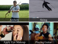
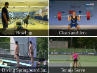
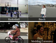
Datasets: Experiments are performed on 5 popular contemporary action recognition and event detection datasets including A Large Human Motion Database (HMDB51) (Kuehne et al, 2011), UCF101 (Soomro et al, 2012), Olympic Sports (Niebles, 2010) and Columbia Consumer Video (CCV) (Jiang et al, 2011). HMDB51 is specifically created for human action recognition. It has 6766 videos from various sources with 51 categories of actions. UCF101 is an action recognition dataset of 13320 realistic action videos, collected from YouTube, with 101 action categories. Olympic Sports is collected from YouTube, and is mainly focused on sports events. It has 783 videos with 16 categories of events. CCV contains 9682 YouTube videos over 20 semantic categories. We illustrate some example frames in Fig. 2. The action/event category names are presented in Table 2. We also evaluate USAA (Fu et al, 2014b) – a subset of CCV specifically annotated with attributes – in order to facilitate comparison against attribute centric ZSL approaches. In addition to above action/event datasets, we also studied a large complex event dataset - TRECVID MED 2013. There are five components to the dataset including Event Kit training, Background training, test set MED, test set Kindred and Research Set. We use standard test set MED for zero-shot testing data and Event Kit as training data.

Table 2: Category names of each dataset.

Dataset	Category Names
HMDB51	brush_hair, cartwheel, catch, chew, clap, climb, climb_stairs, dive, draw_sword, dribble, drink, eat, fall_floor, fencing, flic_flac, golf, handstand, hit, hug, jump, kick, kick_ball, kiss, laugh, pick, pour, pullup, punch, push, pushup, ride_bike, ride_horse, run, shake_hands, shoot_ball, shoot_bow, shoot_gun, sit, situp, smile, smoke, somersault, stand, swing_baseball, sword, sword_exercise, talk, throw, turn, walk, wave
UCF101	Apply Eye Makeup, Apply Lipstick, Archery, Baby Crawling, Balance Beam, Band Marching, Baseball Pitch, Basketball Shooting, Basketball Dunk, Bench Press, Biking, Billiards Shot, Blow Dry Hair, Blowing Candles, Body Weight Squats, Bowling, Boxing Punching Bag, Boxing Speed Bag, Breaststroke, Brushing Teeth, Clean and Jerk, Cliff Diving, Cricket Bowling, Cricket Shot, Cutting In Kitchen, Diving, Drumming, Fencing, Field Hockey Penalty, Floor Gymnastics, Frisbee Catch, Front Crawl, Golf Swing, Haircut, Hammer Throw, Hammering, Handstand Pushups, Handstand Walking, Head Massage, High Jump, Horse Race, Horse Riding, Hula Hoop, Ice Dancing, Javelin Throw, Juggling Balls, Jump Rope, Jumping Jack, Kayaking, Knitting, Long Jump, Lunges, Military Parade, Mixing Batter, Mopping Floor, Nun chucks, Parallel Bars, Pizza Tossing, Playing Guitar, Playing Piano, Playing Tabla, Playing Violin, Playing Cello, Playing Daf, Playing Dhol, Playing Flute, Playing Sitar, Pole Vault, Pommel Horse, Pull Ups, Punch, Push Ups, Rafting, Rock Climbing Indoor, Rope Climbing, Rowing, Salsa Spins, Shaving Beard, Shotput, Skate Boarding, Skiing, Skijet, Sky Diving, Soccer Juggling, Soccer Penalty, Still Rings, Sumo Wrestling, Surfing, Swing, Table Tennis Shot, Tai Chi, Tennis Swing, Throw Discus, Trampoline Jumping, Typing, Uneven Bars, Volleyball Spiking, Walking with a dog, Wall Pushups, Writing On Board, Yo Yo
Olympic Sports	basketball layup, bowling, clean and jerk, discus throw, hammer throw, high jump, javelin throw, long jump, diving platform 10m, pole vault, shot put, snatch, diving springboard 3m, tennis serve, triple jump, vault
CCV	Basketball, Baseball, Soccer, IceSkating, Skiing, Swimming, Biking, Cat, Dog, Bird, Graduation, Birthday, WeddingReception, WeddingCeremony, WeddingDance, MusicPerformance, NonmusicPerformance, Parade, Beach, Playground

(a) HMDB51

(b) UCF101

(c) OlympicSports

(d) $CCV$

Figure 2: Example frames for different action datasets.

Visual Feature Encoding: For each video we extract improved trajectory feature (ITF) descriptors (Wang and Schmid, 2013) and encode them with Fisher Vectors (FV). We first compute ITF with 3 descriptors (HOG, HOF and MBH). We apply PCA to reduce the dimension of descriptors by half which results in descriptors with $198$ dimensions in total. Then we randomly sample 256,000 descriptors from each of the 5 action/event datasets and learn a Gaussian Mixture Model with $128$ components from the combined training descriptors. Finally the dimension of FV encoded feature is equal to $d_{x}=2\times 128\times 198=50688$. The visual feature for TRECVID MED 2013 dataset was extracted using ITF with HOG and MBH descriptors encoded with Fisher Vectors. We use the FV encoded feature provided by Habibian et al (2014b).

Semantic Embedding Space: We adopted the skip-gram neural network model (Mikolov et al, 2013) trained on the Google News dataset (about 100 billion words). This neural network can then encode any of approximately 3 million unique worlds as a $d_{z}=300$ dimension vector.

4.2 Zero-shot Learning on Actions and Events

Data Split: Because there is no existing zero-shot learning evaluation protocol for most existing action and event datasets we propose our own splits. We first propose a 50/50 category split for all datasets. Visual to semantic space mappings are trained on the $50\%$ training categories, and the other $50\%$ are held out unseen for testing time. We randomly generate 50 independent splits and take the mean accuracy and standard deviation for evaluation. Among the 50 splits, all categories are evaluated as testing classes, and the frequency is evenly distributed.

4.2.1 Evaluation of Components

To evaluate the efficacy of each component we considered an extensive combination of blocks including manifold regularizer, self-training, hubness correction and data augmentation. Specifically we evaluated the following options for each component.

• Data Augmentation: Using only within target dataset training data (X) to learn the embedding $f(\mathbf{x})$, or also borrowing data from the auxiliary datasets (✓). (Section 3.2.2). For each of the four datasets HMDB51, UCF101, Olympic Sports and CCV, the other three datasets are treated as the auxiliary sets. Note, there are overlapping categories between the auxiliary and target sets in the sense of exact name match. For instance, the action class Biking exists in both UCF101 and CCV. To avoid violating the zero-shot assumption we exclude these exact matching classes in the auxiliary set. However, we consider that semantic overlaps, e.g. Biking in UCF101 and Ride Bike in HMDB51, should not be excluded because recognizing such paraphrase of action category is the problem to be solved by zero-shot learning and exploiting such semantic relatedness is unique to word-vector embedding approach.

• Embedding: We compare ridge regression (RR) with manifold regularized ridge regression (MR) (Section 3.2).

• Self Training: With (✓) or without (X) self-training before matching (Section 3.3.1).

• Matching Strategy: We compare conventional NN matching (NN) Eq. (13) versus Normalised Nearest Neighbour (NRM) Eq. (15) and Globally Corrected (GC) matching Eq. (17) (Section 3.3.1). Note that the hubness correction methods (NRM and GC) do not change retrieval performance. Therefore, NN/ NRM/ GC do not perform differently on OlympicSports and CCV.

• Transductive: (Trans) Indicating whether the combination of components is transductive (✓) or not (X). The former requires the access to unlabelled testing data.

Based on this breakdown of components, we note that the condition (X-RR-X-NN-X) is roughly equivalent to the methods in Socher et al (2013) and Lazaridou et al (2014), and the conditions (X-RR-X-GC-✓, X-RR-X-NRM-✓) are roughly equivalent to Dinu et al (2015). We present the results in Table 3.

Metrics: HMDB, UCF and USAA are classification benchmarks, so we report average accuracy metric. Olympic Sports and CCV are detection benchmarks, so we report mean average precision (mAP) metrics. We note that because distance normalization (NRM) does not change the relative rank of testing instances w.r.t. testing class, there is no difference between NRM and NN for mAP. Therefore, we insert a ‘$-$’ for Match-NRM on Olympic Sports and CCV. The performance for these ‘$-$’ is the same as their NN counterparts.

Table 3: Evaluation of the contribution of individual component (average % accuracy $\pm$ standard deviation for HMDB51, UCF101 and USAA and mean average precision $\pm$ standard deviation for Olympic Sports and CCV). All ‘$-$’ indicate no difference in performance between NN and NRM.

Model	Match	ST	Data Aug	Trans	HMDB51	UCF101	Olympic Sports	CCV	USAA
RR	NN	X	X	X	14.5$\pm$2.7	11.7$\pm$1.7	35.7$\pm$8.8	20.7$\pm$3.0	29.5$\pm$5.5
RR	NN	✓	X	✓	17.0$\pm$3.1	15.9$\pm$2.3	37.3$\pm$9.1	21.7$\pm$3.2	30.2$\pm$5.2
MR	NN	X	X	✓	15.9$\pm$3.1	12.9$\pm$2.2	37.7$\pm$9.5	21.4$\pm$3.0	29.8$\pm$4.0
MR	NN	✓	X	✓	18.6$\pm$3.9	17.6$\pm$2.7	38.6$\pm$10.6	22.5$\pm$3.4	35.5$\pm$4.0
RR	GC	X	X	✓	15.3$\pm$2.7	13.5$\pm$1.8	35.7$\pm$8.8	20.7$\pm$3.0	26.1$\pm$6.7
RR	GC	✓	X	✓	17.0$\pm$2.9	14.8$\pm$2.0	37.3$\pm$9.1	21.7$\pm$3.2	29.0$\pm$4.0
RR	NRM	X	X	✓	16.1$\pm$2.7	13.9$\pm$1.5	-	-	28.6$\pm$7.2
RR	NRM	✓	X	✓	17.2$\pm$2.9	16.1$\pm$2.2	-	-	28.6$\pm$7.6
MR	NRM	X	X	✓	18.0$\pm$3.2	15.6$\pm$2.0	-	-	28.2$\pm$5.4
MR	NRM	✓	X	✓	19.1$\pm$3.8	18.0$\pm$2.7	-	-	31.6$\pm$3.2
RR	NN	X	✓	X	20.4$\pm$2.9	15.7$\pm$1.6	38.6$\pm$7.5	30.3$\pm$3.9	28.2$\pm$4.6
RR	NN	✓	✓	✓	23.6$\pm$3.7	21.2$\pm$2.4	42.0$\pm$8.2	33.8$\pm$4.7	42.8$\pm$8.7
RR	NRM	X	✓	✓	21.0$\pm$2.7	18.5$\pm$1.7	-	-	35.6$\pm$2.6
RR	NRM	✓	✓	✓	23.7$\pm$3.4	22.2$\pm$2.6	-	-	42.6$\pm$9.1
MR	NN	X	✓	✓	20.6$\pm$2.9	17.2$\pm$1.6	41.1$\pm$7.7	30.4$\pm$3.9	30.3$\pm$4.9
MR	NN	✓	✓	✓	23.5$\pm$3.9	20.6$\pm$2.4	43.2$\pm$8.3	33.0$\pm$4.8	41.2$\pm$9.7
MR	NRM	✓	✓	✓	24.1$\pm$3.8	22.1$\pm$2.5	-	-	43.3$\pm$10.9

Experimental Results: We make the following observations from the results in Table 3: (i) The simplest approach of directly mapping features to the embedding space (X-RR-X-NN-X (Socher et al, 2013; Lazaridou et al, 2014)) works reasonably well suggesting that semantic space is effective as a representation and supports ZSL. (ii) Manifold regularization reliably improves performance compared to conventional ridge regression by reducing the domain shift through considering the unlabelled testing data (transductive learning). (iii) Data augmentation also significantly improves the results by providing a more representative sample of training data for learning the embedding. (iv) In line with previous work self-training (Fu et al, 2015a) and Hubness (Dinu et al, 2015) post-processing improve results at testing time, and this is complementary with our proposed manifold regularization and data augmentation.

4.2.2 Comparison With State-of-the-Art

In addition to the above variants of our framework, we also evaluate the following state-of-the-art approaches to ZSL on action recognition tasks. As both word-vector embedding and manually labelled attributes are widely studied in the literature of zero-shot learning, we compare our approach using both word-vector and attribute semantic embedding with the state-of-the-art models. Attribute embedding is only evaluated on UCF, Olympic Sports and USAA where attributes are available.

Word-Vector Embedding:  For word-vector embedding, we evaluate three alternative models:

1. Structured Joint Embedding (SJE) We use the code of Akata et al (2015) with FV encoded visual feature to evaluate the performance on all 5 datasets. The SJE model employs bilinear ranking to ensure relevant labels (word-vectors) are ranked higher than irrelevant labels.

2. Convex Combination of Semantic Embeddings (ConSE) We implement the ConSE model (Norouzi et al, 2014) with the same FV encoded feature and evaluate on all 5 datasets. The ConSE model firstly trains classifiers for each known category $p(y_{j}|\mathbf{x})$. Given testing visual data $\mathbf{x}$, the semantic embedding of visual data is synthesized by a linear combination of known category embeddings as $f(\mathbf{x})=\sum_{j=1}^{T}p(y_{j}|\mathbf{x})\mathbf{z}_{j}$ where $T$ is the top $T$ known classes.

3. Support Vector Embedding (SVE) Our preliminary model published in Xu et al (2015). This model learns the visual-to-semantic mapping via support vector regression. Performance is reported on HMDB51 and UCF101 datasets.

Attribute Embedding:  In addition to word-vector embedding based methods, we also compare against existing state-of-the-art models using attribute embeddings. To enable direct comparisons with the same embedding, we carry out experiments for our approach with attribute embedding as well (although in this setting our data augmentation cannot be applied). Specifically, we compare the following methods:

1. Direct Attribute Prediction (DAP) We implement the method of Lampert et al (2014), but using the same FV encoded visual features and linear kernel SVM attribute classifiers $p(\mathbf{a}|\mathbf{x})$. Recognition is then performed based on attribute posteriors and manually specified attribute descriptor $p(\mathbf{a}|\mathit{y})$.

2. Indirect Attribute Prediction (IAP) (Lampert et al, 2014). This differs from DAP by learning a per-category classifier $p(\mathit{y}|\mathbf{x})$ from training data first and then use the training category attribute-prototype dependency $p(\mathbf{a}|\mathit{y})$ to obtain attribute estimator $p(\mathbf{a}|\mathbf{x})$.

3. Human Actions by Attributes (HAA) (Liu et al, 2011). We reproduce a simplified version of this model which exploits the manually labelled attributes $\{a_{m}\}$ for zero-shot learning. Similar to DAP, a binary SVM classifier is trained per attribute. In the testing phase, each testing sample is projected into attribute space and then assigned to the closest testing/unknown class based on cosine distance to the class prototype (NN).

4. Propagated Semantic Transfer (PST) (Rohrbach et al, 2013) and (Rohrbach et al, 2016). Label propagation is adopted in this approach to adjust the initial predictions of DAP. Specifically, a KNN graph is constructed in the attribute embedding space and a smoothed solution is obtained transductively by semi-supervised label propagation (Zhou et al, 2004).

5. Multi-Modal Latent Attribute Topic Model (M2LATM) (Fu et al, 2014b). It exploits both user-defined and discovered latent attributes to facilitate zero-shot learning. This model fuses multiple features – static (SIFT), motion (STIP) and audio (MFCC), and thus has an advantage compared to other methods evaluated that use vision alone. We report the results on USAA from Fu et al (2014b).

6. Transductive Multi-View Bayesian Label Propagation (TMV-BLP) (Fu et al, 2014a). This model builds a common space for multiple embeddings. It combines attribute and word-vectors, and applies bayesian label propagation to infer the category of testing instances. It evaluated on USAA dataset with SIFT, STIP and MFCC features.

7. Transductive Multi-View Hypergraph Label Propagation (TMV-HLP) (Fu et al, 2015a). An improved version of TMV-BLP. A distributed hypergraph was adopted to replace the local neighbourhood graph in Fu et al (2014a).

8. Unsupervised Domain Adaptation (UDA). The UDA model (Kodirov et al, 2015) learns dictionary on auxiliary data and adapts it to the target data as a constraint on the target dictionary rather than blindly using the same dictionary.

Mixed Embedding: We refer to exploiting attribute and word-vector embeddings jointly as studied by Fu et al (2015a) and Akata et al (2015). Although multi-view embedding is not the focus of this work, we evaluate our model with a simple concatenation of attribute and word-vector embeddings. Three alternatives are compared including TMV-BLP (Fu et al, 2014a), UDA (Kodirov et al, 2015) and TMV-HLP (Fu et al, 2015a).

Method Properties:  We indicate the nature of each approach with four parameters. DA - if data augmentation is applied. Trans - whether the approach requires transductive access to testing data. Embed - what semantic embedding is used. Embed-A, Embed-W and Embed A+W indicate attribute, word vector, and both attribute+word vector embeddings respectively. Feat - What visual feature is used. FV indicates Fisher vector encoded dense trajectory feature; BoW indicates bag of words encoded dense trajectory feature; and SMS indicates joint SIFT, MFCC and STIP feature.

Table 4: Comparison with state-of-the-art approaches to ZSL. Both attribute and word-vector embeddings are studied for fair comparison. ^∗ performances are estimated from Fig. 2 (a) $\Gamma(X+V)$ and $\Gamma(X+A)$ respectively in Fu et al (2014a). ^∗∗ performances are estimated from Fig. 5 (c) $\Gamma(X+V)$ and $\Gamma(X+A)$ respectively in Fu et al (2015a). N/A indicates not available due to the absence of attribute annotation or not reported by the original work.

Model	DA	Trans	Embed	Feat	HMDB51	UCF101	Olympic Sports	CCV	USAA
Random Guess	X	X	X	X	4.0	2.0	12.5	10.0	25.0
RR (Ours)	X	X	W	FV	14.5$\pm$2.7	11.7$\pm$1.7	35.7$\pm$8.8	20.7$\pm$3.0	29.5$\pm$5.5
MR (Ours)	X	✓	W	FV	19.1$\pm$3.8	18.0$\pm$2.7	38.6$\pm$10.6	22.5$\pm$3.4	31.6$\pm$3.2
MR (Ours)	✓	✓	W	FV	24.1$\pm$3.8	22.1$\pm$2.5	43.2$\pm$8.3	33.0$\pm$4.8	43.3$\pm$10.9
SJE (Akata et al, 2015)	X	X	W	FV	12.0$\pm$2.6	9.3$\pm$1.7	34.6$\pm$7.6	16.3$\pm$3.1	21.3$\pm$0.6
ConSe (Norouzi et al, 2014)	X	X	W	FV	15.0$\pm$2.7	11.6$\pm$2.1	36.6$\pm$9.0	20.7$\pm$3.1	28.2$\pm$4.8
TMV-BLP (Fu et al, 2014a)∗	X	✓	W	SMS	N/A	N/A	N/A	N/A	41.0
TMV-HLP (Fu et al, 2015a)∗∗	X	✓	W	SMS	N/A	N/A	N/A	N/A	43.0
SVE (Xu et al, 2015)	X	X	W	BoW	12.9$\pm$2.3	11.0$\pm$1.8	N/A	N/A	N/A
RR (Ours)	X	X	A	FV	N/A	12.6$\pm$1.8	51.7$\pm$11.3	N/A	44.2$\pm$13.9
MR (Ours)	X	✓	A	FV	N/A	20.2$\pm$2.2	53.5$\pm$11.9	N/A	51.6$\pm$10.0
DAP (Lampert et al, 2014)	X	X	A	FV	N/A	15.2$\pm$1.9	44.4$\pm$9.9	N/A	37.9$\pm$5.9
IAP (Lampert et al, 2014)	X	X	A	FV	N/A	15.6$\pm$2.2	44.0$\pm$10.7	N/A	31.7$\pm$1.6
HAA (Liu et al, 2011)	X	X	A	FV	N/A	14.3$\pm$2.0	48.3$\pm$10.2	N/A	41.2$\pm$9.8
PST (Rohrbach et al, 2013)	X	✓	A	FV	N/A	15.3$\pm$2.2	48.6$\pm$11.0	N/A	47.9$\pm$10.6
M2LATM (Fu et al, 2014b)	X	✓	A	SMS	N/A	N/A	N/A	N/A	41.9
TMV-BLP (Fu et al, 2014a)∗	X	✓	A	SMS	N/A	N/A	N/A	N/A	40.0
TMV-HLP (Fu et al, 2015a)∗∗	X	✓	A	SMS	N/A	N/A	N/A	N/A	42.0
UDA (Kodirov et al, 2015)	X	✓	A	FV	N/A	13.2$\pm$1.9	N/A	N/A	N/A
MR (Ours)	X	✓	A+W	FV	N/A	20.8$\pm$2.3	53.2$\pm$11.6	N/A	51.9$\pm$10.1
TMV-BLP (Fu et al, 2014a)	X	✓	A+W	SMS	N/A	N/A	N/A	N/A	47.8
UDA (Kodirov et al, 2015)	X	✓	A+W	FV	N/A	14.0$\pm$1.8	N/A	N/A	N/A
TMV-HLP (Fu et al, 2015a)	X	✓	A+W	SMS	N/A	N/A	N/A	N/A	50.4

Experimental Results: The full results are presented in Table 4, from which we draw the following conclusions: (i) Our non-transductive model (RR) is strong compared with alternative models with either word-vector embedding or attribute embedding. For example, our RR model is able to beat SJE and ConSE in UCF101, CCV and USAA with word-vector embedding and beat DAP, IAP and HAA in Olympic Sports and USAA. (ii) With transductive access to testing data, our model MR-X-✓-W is better than most alternative models with word-vector and competitive against models with attribute embedding. (iii) The overall combination of all components, manifold regularized regression (MR), Data Augmentation (DA) and Self-training and hubness (Trans), with word-vector embedding (MR-✓-✓-W) can yield very competitive performance. Depending on the dataset, our overall model is comparable or significantly better than the attribute-centric methods, e.g. UCF101. (iv) With mix-embedding (A+W) our model is still very competitive against existing ZSL approaches and outperform TMV-BLP, UDA and TMV-HLP. Apart from the above observations we note that the ZSL performance variance is relatively high, particularly in Olympic Sports and USAA datasets. This is because specific choice of train/test classes in ZSL matters more than specific choice of train/test instances in conventional supervised learning. E.g., in olympic sports there are highly related categories ‘high jump’ - ‘long jump’ and ‘diving platform 10m’ - ‘diving springboard 3m’. Recognition performance is higher when these pairs are separated in training and testing, and lower if they are both in testing. This issue is explored further in Sec. 4.5

4.2.3 Generalising the Transductive Setting

In this section, we study the possibility to apply the transductive learning ideas investigated here to improve existing zero-shot learning approaches with both word-vector and attribute embeddings. In particular we consider transductive generalisations of three alternative models SJE, ConSE and HAA.

SJE:   SJE (Akata et al, 2015) uses a bi-linear mapping to evaluate the compatibility between novel instances and word-vectors. Suppose we have the bi-linear form $\mathbf{x}^{\top}\mathbf{W}\mathbf{z}$ to compute the compatibility score between category name word-vector $\mathbf{z}$ (output embedding) and video instance $\mathbf{x}$ (input embedding) which corresponds to Eq (1) in Akata et al (2015). Given learned model $\mathbf{W}$ we can first project video instance by this mapping as $\mathbf{x}^{\top}\mathbf{W}$. Then we can apply self-training to adjust the novel category’s output embedding $\mathbf{z}$ as,

$$\tilde{\mathbf{z}}=\frac{1}{|NN_{k}(\mathbf{z})|}\sum\limits_{i\in NN_{k}(\mathbf{z})}(\mathbf{x}_{i}^{\top}\mathbf{W})$$ (18)

where the function $NN_{k}(\cdot)$ returns the k nearest neighbour of $\mathbf{z}$ w.r.t. all testing video instances $\{\mathbf{x}_{i}^{\top}\mathbf{W}\}$. The adjusted category embedding replaces the original output embedding for prediction. We can resolve the hubness issue for bi-linear model as well. Specifically, we use the $1-\mathbf{x}^{\top}\mathbf{W}\mathbf{z}$ normalised to between 0 and 1 as the distance and apply the same distance normalization trick introduced in Eq (15).

ConSE:  We train SVM classifiers for each known category as $p(y_{j}|\mathbf{x})$ and take the top $T$ responses for a testing instance to synthesize the embedding as,

$$f(\mathbf{x_{i}})=\frac{1}{T}\sum\limits_{j=1}^{T}p(y_{j}|\mathbf{x}_{i})\mathbf{z}_{j}$$ (19)

where $\mathbf{z}_{j}$ is the semantic embedding of $j$-th known category. To apply self-training, we simply do the same calculation w.r.t. embeddings of testing videos as,

$$\tilde{\mathbf{z}}=\frac{1}{|NN_{k}(\mathbf{z})|}\sum\limits_{i\in NN_{k}(\mathbf{z})}f(\mathbf{x}_{i})$$ (20)

Hubness correction can be integrated in the same way.

HAA:  We do nearest neighbour matching in attribute embedding space, so both self-training and hubness correction can be applied in the same ways as our model.

Table 5: Study the possibility to generalize transductive settings to existing zero-shot learning approaches.

Model	Match	ST	Trans	Embed	Feat	HMDB51	UCF101	Olympic Sports	CCV	USAA
SJE	NN	X	X	W	FV	12.0$\pm$2.6	9.3$\pm$1.7	34.6$\pm$7.6	16.3$\pm$3.1	21.3$\pm$0.6
SJE	NN	✓	✓	W	FV	10.5$\pm$2.4	8.9$\pm$2.2	32.5$\pm$6.7	15.4$\pm$3.1	27.7$\pm$7.1
SJE	NRM	X	✓	W	FV	12.7$\pm$2.4	10.5$\pm$1.7	-	-	19.8$\pm$6.7
SJE	NRM	✓	✓	W	FV	10.6$\pm$2.3	9.2$\pm$2.0	-	-	26.8$\pm$9.2
ConSE	NN	X	X	W	FV	15.0$\pm$2.7	11.6$\pm$2.1	36.6$\pm$9.0	20.7$\pm$3.1	28.2$\pm$4.8
ConSE	NN	✓	✓	W	FV	15.4$\pm$2.8	12.7$\pm$2.2	37.0$\pm$9.9	21.2$\pm$3.1	28.3$\pm$4.2
ConSE	NRM	X	✓	W	FV	15.8$\pm$2.6	12.7$\pm$2.1	-	-	26.2$\pm$9.5
ConSE	NRM	✓	✓	W	FV	16.3$\pm$3.1	12.9$\pm$2.2	-	-	26.3$\pm$9.4
HAA	NN	X	X	A	FV	N/A	14.3$\pm$2.0	48.3$\pm$10.2	N/A	41.2$\pm$9.8
HAA	NN	✓	✓	A	FV	N/A	18.7$\pm$2.4	49.4$\pm$10.8	N/A	47.6$\pm$10.5
HAA	NRM	X	✓	A	FV	N/A	15.9$\pm$1.9	-	N/A	48.4$\pm$8.9
HAA	NRM	✓	✓	A	FV	N/A	19.1$\pm$2.3	-	N/A	49.4$\pm$9.0

Experimental Results: The results on generalizing other methods to the transductive setting are presented in Table 5. We observe that hubness correction (NRM) improves performance on HMDB51 and UCF101 for all three models. The effect is not so clear on USAA except for HAA. As hubness correction does not change the rank of individual testing instances w.r.t. testing category, no improvement is expected on Olympic Sports and CCV from NN to NRM. Self-training is in general effective for ConSE and HAA but is detrimental to SJE. This may be due to SJE’s ranking loss: It aims to rank, rather than project video instances to the vicinity of their category embedding. Therefore, the projected video instances ($\mathbf{x}^{\top}\mathbf{W}$) do not form neat clusters in the word-vector space which makes self-training ineffective.

4.3 Zero-shot Learning of Complex Events

In this section, we experiment on the more challenging complex event dataset - TRECVID MED 2013.

Data Split: We study the 30 classes of the MED test set, holding out the 20 events specified by the 2013 evaluation scheme for zero-shot recognition, and training on the other 10. We train on the total 1611 videos in Event Kit Train (160 per event in average) and test on the 27K examples in MED test, of which only about 1448 videos are the 20 events to be detected. This is different to the standard TRECVID MED 2013 0EK in which concept detectors are trained on the Research Set (Habibian et al, 2014b, a; Wu et al, 2014). This experimental design is chosen because we want to exploit only per-category annotation (event name) as semantic supervision, rather than requiring the per-video sentence annotation used in the Research Set which is very expensive to collect. We note that with few exceptions (Jain and Snoek, 2015) TRECVID MED 2013 is rarely addressed with event name annotation only. With this assumption, it means we use fewer training videos (1611) compared to the 10K video Research Set. Thus our results are not comparable to existing TRECVID MED 2013 0EK benchmark results, because we use vastly less training data.

Table 6: Events for training visual to semantic regression

ID	Event Name	ID	Event Name
E001	Attempting a board trick	E002	Feeding an animal
E003	Landing a fish	E004	Wedding ceremony
E005	Working on a woodworking project	E016	Doing homework or studying
E017	Hide and seek	E018	Hiking
E019	Installing flooring	E020	Writing

Table 7: Events for testing zero-shot event detection

ID	Event Name	ID	Event Name
E006	Birthday party	E007	Changing a vehicle tire
E008	Flash mob gathering	E009	Getting a vehicle unstuck
E010	Grooming an animal	E011	Making a sandwich
E012	Parade	E013	Parkour
E014	Repairing an appliance	E015	Working on a sewing project
E021	Attempting a bike trick	E022	Cleaning an appliance
E023	Dog show	E024	Giving directions to a location
E025	Marriage proposal	E026	Renovating a home
E027	Rock climbing	E028	Town hall meeting
E029	Winning a race without a vehicle	E030	Working on a metal crafts project

Baselines: We compare 5 alternative baselines for TRECVID MED zero-shot event detection.

1. Random Guess - Randomly rank the candidates.

2. NN (X-RR-X-NN-X). Rank videos with $l_{2}$ distance in the semantic space.

3. NN + ST (X-RR-✓-NN-✓). Adjust prototypes with self-training.

4. Manifold (X-MR-X-NN-✓). Add manifold regularization term in the visual to semantic regression model.

5. Manifold + ST (X-MR-✓-NN-✓) - manifold regularization regression with self-training.

We were not able to investigate data augmentation for TRECVID due to the different feature encoding from the other action datasets.

We present the performance of zero-shot learning on TRECVID MED 2013 in Fig. 3 and Table 8. Fig. 3 reports the performance of 4 alternative models and random guess baseline in detecting 20 events in mean average precision (mAP) and the average over all events (Average). Compared to Random Guess ($0.28\%$), our direct embedding approach (NN) is effective at zero-shot video detection. Self-Training and Manifold Regularization further improve the performance. Table 8 puts the results in broader context by summarising them in terms of absolute performance.

Figure 3: Zero-shot performance on TRECVID MED 2013 measured in mean average precision (mAP).

Table 8: Event detection performance on TRECVID MED 2013. mAP across 20 events to be detected.

Embed	ST	Match	Average mAP
RR	X	NN	$1.18\%$
RR	✓	NN	$1.25\%$
MR	X	NN	$1.22\%$
MR	✓	NN	$1.38\%$
Random Guess			$0.28\%$

4.4 Zero-Shot Qualitative Visualization

In this section we illustrate qualitatively the effect of our contributions on the resulting embedding space matching problem. For visualisation, we randomly sample 5 testing classes from HMDB51 and project all samples from these classes into the semantic space by (i) conventional ridge regression; (ii) manifold regularized regression and (iii) manifold regularized ridge regression with data augmentation. The results are visualised in 2D in Fig. 4 with t-SNE (Maaten and Hinton, 2008). Three sets of testing classes are presented for diversity. Data instances are shown as dots, prototypes (class name projections) as diamonds, and self-training adapted prototypes as stars. Colours indicate category.

(a) Category set 1

(b) Category set 2

(c) Category set 3

Figure 4: A qualitative t-SNE illustration of ZSL with semantic space representation for random testing class subsets (a), (b) and (c). Variants: ridge regression, manifold regression and data augmented manifold regression. Dots indicate instances, color categories, and star/diamond show category prototypes with/without self-training.

There are three main observations from Fig. 4: (i) Manifold regularized regression yields better visual semantic projections as instances of the same class tend to form tighter clusters. This is due to the constraint of preserving the manifold structure from the visual feature space. (ii) Data augmentation yields an even more accurate projection of unseen data, as instances are projected closer to the prototypes and classes are more separable. (iii) Self-training is effective as the adapted prototypes (stars) are closer to the center of the corresponding samples (dots) than the original prototypes (diamonds). These observations illustrate the mechanism of our ZSL accuracy improvement on conventional approaches.

These qualitative illustrations also give intuition about why the previous result in Fig 3 is one of a moderate overall increase in mean AP that is the result of a varied impact of the AP for individual classes. Depending on the data and initial prototype positions, the self-training sometimes makes a very effective adjustment to the prototypes, and other times it makes little adjustment to the prototype, and hence that class’ AP. E.g., In Fig. 4(a), Augmented: compare blue/yellow classes versus red class.

4.5 Understanding ZSL and Predicting Transferrability

In this section we present further insight into considerations on what factors will affect the efficacy of ZSL, through a category-level analysis. The basic assumption of ZSL is that the embedding $f(\mathbf{x})$ trained on known class data, will also apply to testing classes. As we have discussed throughout this study, this assumption is stretched to some extent due to the disjoint training and testing category sets. This leads us to investigate how zero-shot performance depends on the specific choice of training classes and their relation to the held out testing classes.

Impact of training class choice on testing performance: We first investigate whether there are specific classes which, if included as training data, significantly impact testing class performance. To study this, we compute the correlation between training class inclusion and testing performance. Specifically, we consider a pair of random variables $\{b^{tr}_{i},e^{te}_{j}\}$ where $b^{tr}_{i}$ is a binary scalar indicating if the $i$th class is in the training set and $e_{j}$ is the recognition accuracy of the $j$th testing class. We compute the correlation $corr(i,j)$ between every pair of variables over the 50 random splits:

$$corr(i,j)=\frac{\mathbb{E}[({b}^{tr}_{i}-\overline{{b}^{tr}_{i}})({e}^{te}_{j}-\overline{e^{te}_{j}})]}{var(b^{tr}_{i})var(e^{te}_{j})}.$$ (21)

We use chord diagrams to visualize the relation between categories in Fig 5(a). The strength of positive cross-category correlation is indicated by the width of the bands connecting the categories on the circle. I.e., a wide band indicates inclusion of one category as training data facilitates the zero-shot recognition of the other.

(a) HMDB51 class correlation

(b) HMDB51 class name affinity

(c) Olympic Sports class correlation

(d) Olympic Sports class name affinity

Figure 5: Chord Diagram to illustrate the category correlation discovered from zero-shot recognition experiments. (a) and (c) illustrate the correlation discovered from 50 random split zero-shot experiments; (b) and (d) illustrate the class name affinity in word-vector embedding space measured as cosine similarity.

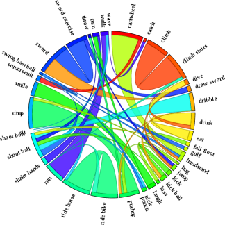
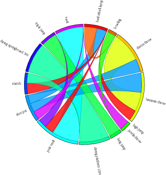
We can make several qualitative observations from the chord diagrams. The class correlation captures the dependence of category B’s recognition rate on category A’s presence in the training set. So for instance for A=ride horse and B=ride bike, Fig. 5(a) shows that we would expect high recognition accuracy of ride horse if ride bike is present in training set and vice versa. However while cartwheel supports the recognition of handstand, the reverse is not true.

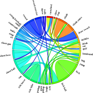
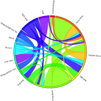
Cross-class transferability correlates with word-vector similarity: We next investigate the affinity between class names’ vector representations, and cross-class transferability. Class name affinities are shown in Fig 5(b) as chord diagrams. Visually there is some similarity to the cross-class transferability presented in Fig 5(a). To quantify this connection between transfer efficacy and classname relatedness, we vectorise the correlation (Fig 5(a)) and class name affinity (Fig 5(b)) matrices ($51\times 51$) into 2601 dim vectors and then compute the correlation coefficients between the two vectors. The correlation is $0.548$, suggesting that class name relatedness and efficacy for ZSL are indeed connected. This is to say, if class A is present in training set and class B in testing set, and A has high affinity with B in word-vector distance measure, we could expect high performance in recognizing class B.

To qualitatively illustrate this connection, we list the top 10 positively correlated category pairs in Table 9. Here the correlation of action 1 being in training and action 2 in testing is given as Fwd Corr, with Back Corr being the opposite. The affinity between category names are given as WV Aff which is defined as percentile rank of word-vector distance (closer to 1 means more similar). Clearly highly correlated categories have higher word-vector similarity.

Table 9: Top 10 positive correlated class pairs

Action 1	Action 2	Fwd Corr	Back Corr	WV Aff
climb stairs	climb	0.94	0.92	0.98
ride horse	ride bike	0.95	0.91	0.98
situp	pushup	0.96	0.79	0.91
sword exercise	sword	0.87	0.85	0.98
handstand	cartwheel	0.62	0.96	0.97
eat	drink	0.75	0.81	0.96
smile	laugh	0.82	0.72	0.97
walk	run	0.61	0.90	0.96
shoot ball	dribble	0.52	0.87	0.97
sword	draw sword	0.86	0.45	0.98

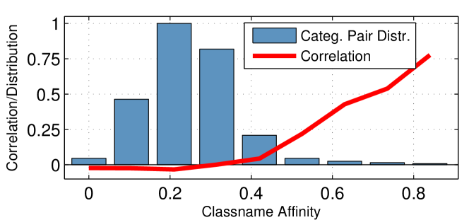
Although zero-shot transfer overall is effective, there are also some individual negative correlations. We illustrate the distribution of positive and negative transfer outcomes in Fig. 6. Here we sort all the class pairings into ten bins by their name affinity and plot the resulting histogram (blue bars). Clearly the majority of pairs have low classname affinity. For each bin of class-pairs, we also compute their average correlation defined in Eq 21 (Fig. 6, red line). There are a few observations to be made: (i) Class name affinity is clearly related to positive correlation: the correlation (red line) goes up significantly for high-affinity class pairs. (ii) There are a relatively small number of category pairs that account for the high positive correlation outcomes (low blue bars to the right). This suggests that overall ZSL efficacy is strongly impacted by the presence of key supporting classes in the training set. (iii) There are a larger number of category pairs which exhibit negative transferability (red correlation is negative around affinity of 0.2). However negative transfer effects are quantitatively weak compared to positive transfer (red correlation line gets only weakly negative but strongly positive).

Figure 6: The connection between transfer efficacy and classname affinity: Illustrated by class correlation v.s. class name affinity.

Predicting Transferability: Based on the previous observations we hypothesize that class name affinity is predictive of ZSL performance, and may provide a guide to selecting a good set of training classes to maximise ZSL efficacy. This is desirable in real application as it is often beneficial to best utilize the limited availability to annotate most useful training data for the recognition of novel categories. We formally define the problem as given fixed testing categories $\{\mathit{y}_{j}|\mathit{y}_{j}\in\mathbf{y}_{te}\}$, we find the $S\%$ subset of training categories $\{\mathit{y}_{i}|\mathit{y}_{i}\in\mathbf{y}_{tr}\}$ which maximize the performance of recognizing testing classes based on their affinity to the testing classes. We first of all explore three alternative (point-to-set) distances to measure the affinity of each training class $\mathit{y}_{i}$ to the set of testing classes $\{\mathit{y}_{j}|\mathit{y}_{j}\in\mathbf{y}_{te}\}$, specifically the maximal/mean/minimal class name affinity:

$$\begin{split}&R_{max}(\mathit{y}_{i},\mathbf{y}_{te})=\underset{\mathit{y}_{j}\in\mathbf{y}_{te}}{\mathrm{max}}\left(1-||g(\mathit{y}_{i})-g(\mathit{y}_{j})||\right)\\ &R_{mean}(\mathit{y}_{i},\mathbf{y}_{te})=\underset{\mathit{y}_{j}\in\mathbf{y}_{te}}{\mathrm{mean}}\left(1-||g(\mathit{y}_{i})-g(\mathit{y}_{j})||\right)\\ &R_{min}(\mathit{y}_{i},\mathbf{y}_{te})=\underset{\mathit{y}_{j}\in\mathbf{y}_{te}}{\mathrm{min}}\left(1-||g(\mathit{y}_{i})-g(\mathit{y}_{j})||\right)\end{split}$$ (22)

These metrics provide a plausible means to quantify the relevance of any potential training class to the testing set. We explore their ability to predict transferability and hence construct a good training set for a particular set of testing classes.

For this experiment, we use HMDB51 with the same 50 random splits introduced in Section 4.2. Keeping the testing sets fixed, we train two alternative models based on different subsets of each training split. Specifically: (1) Related Model selects the top $S\%$ most related training classes (high affinity measure by $R(\mathit{y}_{i},\mathbf{y}_{te})$) to the testing set defined by relatedness measure in Eq. (22) in order to learn the mapping; while (2) Unrelated Model selects the most $100-S\%$ unrelated. Fig. 7 shows the performance of both models as $S$ varies between 0 and 100, where Related selects the top $S\%$ and Unrelated the bottom $100-S\%$. Note that when $S=0\%$ and $S=100\%$ the Unrelated and Related models both select all training classes. Both are then equivalent to the standard ZSL model X-RR-X-NN-X introduced in Table 3. We illustrate the performance of both models and three alternative training-to-testing affinity measures in Fig. (7).

(a) Maximal class name affinity

(b) Mean class name affinity

(c) Minimal class name affinity

Figure 7: Testing the ability to predict ZSL class transferability by class name affinity: A comparison of models selecting related versus un-related classes as training data.

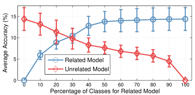
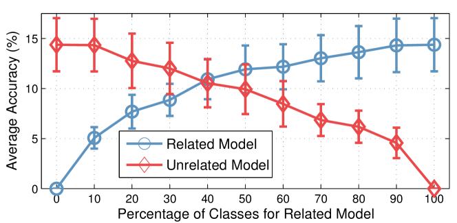
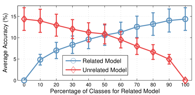
The main observations are as follows: (i) A crossover happens at $30\%$ for maximal class name affinity, which means the model learned on the $30\%$ subset of related training classes outperforms the model learned on the much larger $70\%$ of unrelated classes. (ii) The maximal class name affinity is most predicative on the efficacy of zero-shot learning as (1) the crossover point is the left most among all three alternative strategies, and (2) at the equal data point (50%) the related model most clearly outperforms the unrelated model. (iii) For maximal affinity, as more classes are included the related model increases in performance more rapidly than the unrelated one, and saturates after the top $50\%$ are included. All these observations together indicate that given limited labelling availability, including training classes that are related to testing ones can benefit ZSL performance (as the crossover is to the left of $50\%$).

4.6 Zero-Shot Recognition with Old and New Classes

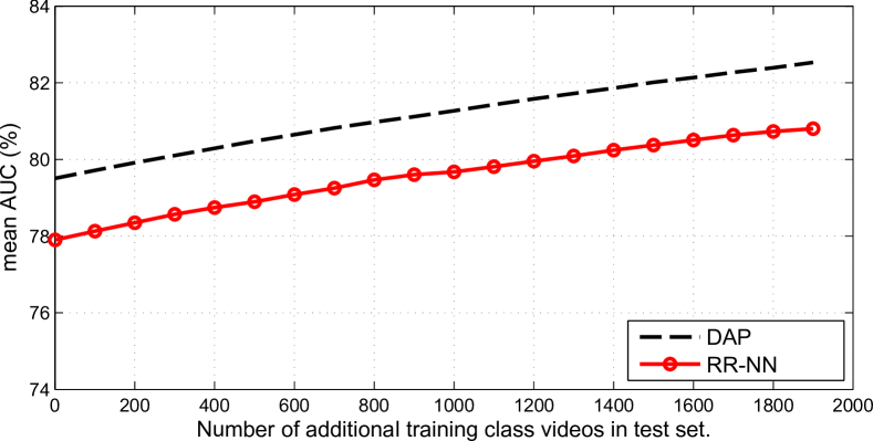
Few existing zero-shot learning studies investigate the ability to recognise novel-category visual instances if they occur among known-class instances at testing time. But this may be the setting under which ZSL is used in real applications. To evaluate how our model performs in the situation where testing instances are mixed with data from training classes, we follow the protocol proposed in Rohrbach et al (2010). Specifically, we choose the first data split from UCF101 dataset and hold out 0-1900 training videos evenly from each training/known class for testing. ZSL models are then trained on the reduced training set. In the testing phase, we label all the held-out training videos as negatives of all testing classes and evaluate AUC for each testing class. We compare two models: (1) attribute-based model (DAP) used in Rohrbach et al (2010); and (2) our direct similarity based prediction (RR-NN) which corresponds to the final model without data augmentation introduced in Table 3. By increasing the number of distractor training videos, we observe from Fig. 8 a steady increase of mean AUC for both attribute-based approach (DAP) and our direct similarity matching (RR-NN). This suggests that both DAP and our model are fairly robust when novel classes must be detected among a background of known classes.

Figure 8: Injecting training/known class samples to testing set.

4.7 Imbalanced Test Set

Transductive strategies have been studied by many existing works (Fu et al, 2015a; Dinu et al, 2015), however none of these works have ever studied the assumptions of test set for successful transductive ZSL. In particular, we note that, in zero-shot scenarios, testing categories could be highly imbalanced. How does the transductive strategies generalize to imbalanced test set remains an untouched problem. To verify this aspect, we carry out a particular experiment. Specifically, we experiment on the first split of HMDB51 and randomly subsample $P\%$ testing data from each of the first 12 testing categories for ZSL evaluation. We illustrate the distribution of testing videos per category for $P=10,50,90$ in Fig. 9.

Figure 9: Distribution of testing videos after subsampling.

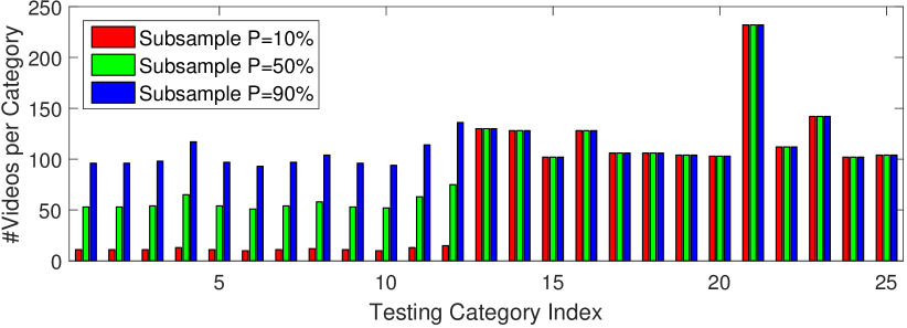
Then we experiment the baseline model - NN and two transductive variants - NN+ST and NN+NRM. By increasing $P$ from 10 to 90 we observe from Fig. 10 that both self-training (red) and hubness correction (green) improve consistently over non-transductive baseline (black dashed). This suggests our transductive strategies are robust to imbalanced test set.

Figure 10: Performance of ZSL for subsampled imbalanced test set.

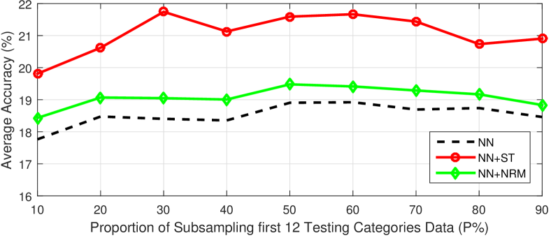
4.8 Multi-Shot Learning

We have thus far focused on the efficacy of unsupervised word-vector embeddings for zero-shot learning. In this section we verify that the same representation also performs comparably to state-of-the-art for standard supervised (multi-shot) action recognition. We use the standard data splits and evaluation metrics for all 4 datasets.

Alternatives: We compare our approach to:

1. Low-Level Feature (Wang and Schmid, 2013) the state-of-the-art results based on low-level features.

2. Human-Labelled Attribute (HLA) (Zheng and Jiang, 2014) Exploits an alternative semantic space using human labelled attributes. The model trains binary linear SVM classifiers for attribute detection and uses the vector of attribute scores as a representation. A SVM classifier with RBF kernel is then trained on attribute representation to predict final labels.

3. Data Driven Attribute (DDA) (Zheng and Jiang, 2014) Learns attributes from data using dictionary learning. These attributes are complementary to the human labelled ones. Automatically discovered attributes are processed in the same way as HLA for action recognition.

4. Mixed attributes (Mix) (Zheng and Jiang, 2014) A combination of HLA and DDA is applied to exploit the complementary information in two attribute sets.

5. Semantic embedding model (Embedding) first learns a word-vector embedding based on regularized linear regression, as in ZSL. But the standard supervised learning data-split is adopted. All data are mapped into the semantic space via regression and a linear SVM classifier is trained for each category with the mapped training data.

The resulting accuracies are shown in Table 10. We observe that our semantic embedding is comparable to the state-of-the-art low-level feature-based classification and is comparable or slightly better than the conventional attribute-based intermediate representations despite the fact that no supervised manual attribute definition and annotation is required.

Table 10: Standard supervised action recognition. Average accuracy for HMDB51 and UCF101 datasets. Mean average precision for Olympic Sports and CCV.

Method	HMDB51	UCF101	Olympic Sports	CCV
Low-Level Feature (Wang and Schmid, 2013)	58.4	84.6	92.1	68.0
HLA (Zheng and Jiang, 2014)	-	81.7	-	-
DDA (Zheng and Jiang, 2014)	-	79.0	-	-
Mix (Zheng and Jiang, 2014)	-	82.3	-	-
Embedding	56.4	82.0	93.4	51.6

4.9 Efficiency and Runtime

Our ZSL algorithm is easy to implement and has favourable efficiency. We estimate the computation complexity for solving manifold regularized regression in Eq (9) to be $O(2N^{3}+d_{z}N)$ (assume the schoolbook matrix multiplication algorithm). Nevertheless, if the number of training data $N$ is too large to fit into memory, our model can be solved by stochastic gradient descent (SGD). The gradient w.r.t. mapping $\mathbf{A}$ is

$$\begin{split}\nabla\mathbf{A}=&\frac{1}{n_{l}}\left(-2\tilde{\mathbf{z}_{i}}\mathbf{k}_{i}^{\top}\mathbf{J}+2\mathbf{A}\mathbf{k}_{i}\mathbf{J}\mathbf{k}_{i}^{\top}\right)\\ &+2\gamma_{A}\mathbf{A}\mathbf{k}_{i}+\frac{\gamma_{I}}{(n_{l}+n_{u})^{2}}2\mathbf{A}\mathbf{k}_{i}\mathbf{l}_{i}^{\top}\mathbf{K}^{\top}\end{split}$$ (23)

for which we estimate the computation complexity for each iteration to be $O(4d_{z}+N^{2})$.

In our implementation, it takes about 300 seconds (including overhead) to train and test on 50 splits of the entire HMDB51 benchmark dataset (6766 videos of 51 categories of actions), or 520 seconds with data augmentation, using a server with 32 Intel E5-2680 cores. The runtime is dominated by the matrix inversion in Eq. (9).

5 Detailed Parameter Sensitivity Analysis

In the main experiments we set the free parameters ridge regularizor $\gamma_{A}=10^{-6}$, manifold regularizor $\gamma_{I}=40$, manifold Knn graph $N^{G}_{K}=5$, Self-Training Knn $N^{st}_{K}=100$. In this section we analyse the impact of these free parameters in our model.

5.1 word-vector Dimension

We investigate how the specific word-vector model $\mathbf{z}=g(\mathit{y})$ affects the performance of our framework. For the study of word-vector dimension we train word-vectors on 4.6M Wikipedia documents and vary dimension from 32 to 1024. We then evaluate the performance of zero-shot and multishot learning v.s. different dimension of embedding space. The results are given in Fig. 11.

Figure 11: Zero-shot performance v.s. dimension of word-vector.

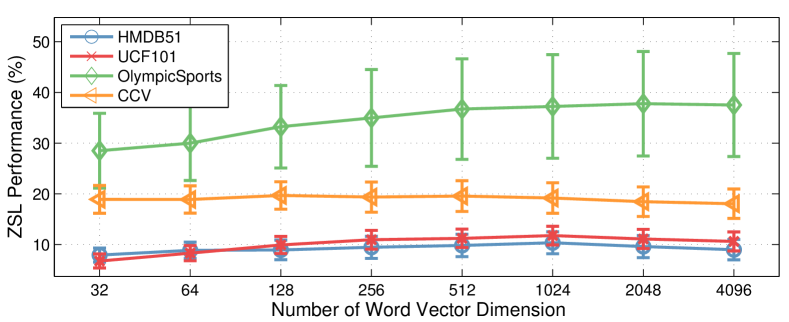
We observe that word-vector dimension does affect the zero-shot recognition performance. Performance generally increases with dimension of word-vector from 32 to 4096 in HMDB51, UCF101 and Olympic Sports, while showing no clear trend for CCV. In general a reasonable word-vector dimension is between 256 to 2048.

5.2 Visual to Semantic Mapping

Ridge regression regularization: We learn the visual to semantic mapping with regularized linear regression. The regularization parameter $\gamma_{A}$ controls the regression model complexity. Here, we study the impact of $\gamma_{A}$ on zero-shot performance. We measure the 50 splits’ average accuracy by varying $\gamma_{A}$ in the range of $\{0,10^{-9},10^{-8},\cdots,10^{-3}\}$. A plot of zero-shot mean accuracy v.s. regularization parameter is given in Fig. 12. From this figure we observe that our model is insensitive to the ridge parameter for any non-zero regularizer. However, when no regularization is used the performance is close to random. This is due to all zero or co-linear rows/columns in the kernel matrix which causes numerical problems in computing the inverse.

Figure 12: Zero-shot mean accuracy v.s. ridge regression parameter

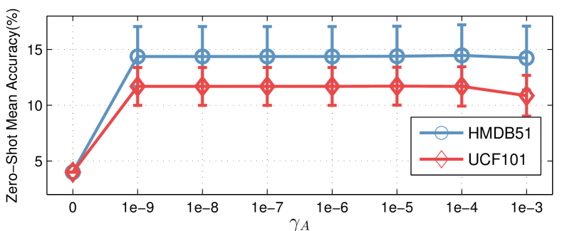
Manifold regression: We have seen that transductively exploiting testing/unlabelled data in manifold learning improves zero-shot performance. Two parameters are involved: the manifold regularization parameter $\gamma_{I}$ in Loss function (Eq. 8) and $N^{G}_{K}$ in constructing the symmetrical KNN graph. $\gamma_{I}$ controls the preference for preserving the manifold structure in mapping to the semantic space, versus exactly fitting the training data. Parameter $N^{G}_{K}$ determines the precision in modelling the manifold structure. Small $N^{G}_{K}$ may more precisely exploit the testing data manifold, however it is more prone to noise in the neighbours.

(a) HMDB51

(b) UCF101

Figure 13: Zero-shot recognition accuracy with respect to manifold regression parameters $\gamma_{I}$ and $N^{G}_{K}$.

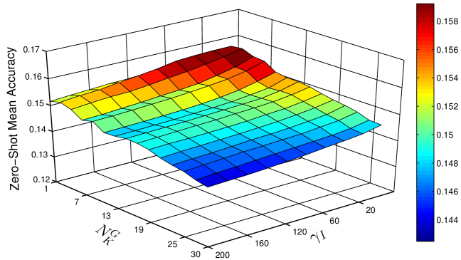
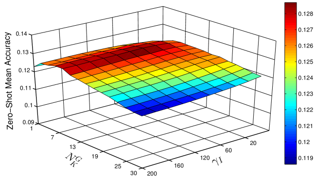
Here we analyse the impact of these two parameters, $\gamma_{I}$ and $N^{G}_{K}$ by measuring zero-shot recognition accuracy on HMDB51 and UCF101. We evaluate the joint effect of $\gamma_{I}$ and $N^{G}_{K}$ while fixing $\gamma_{A}=10^{-6}$. Specifically we test $\gamma_{I}\in\{20,40,\cdots,100\}$ and $N^{G}_{K}\in\{1,3,5\cdots,29\}$. The results in Fig. 13 show that there is a slightly preference towards moderately low values of $N^{G}_{K}$ and $\gamma_{I}$, but the framework is not very sensitive to these parameters.

5.3 Self-Training

We previously demonstrated in Table 3, that self-training (Section 3.4) helps to mitigate the domain shift problem. Here, we study the influence of the $N^{st}_{K}$ parameter for KNN in self-training. Note the $N^{st}_{K}$ concerns the neighbouring data distribution around prototypes at testing time rather than manifold regularization KNN graph $N^{G}_{K}$ at training time. We evaluate
$N^{st}_{K}\in\{1,2,3,\cdots,200\}$. To thoroughly examine the effectiveness of self-training, we investigate all baselines with self-training introduced in section 4.2 including

• X-RR-✓-NN-✓   (NN+ST)

• X-RR-✓-NRM-✓  (NRM+ST)

• X-RR-✓-GC-✓   (GC+ST)

• X-MR-✓-NN-✓   (Manifold+ST)

• X-MR-✓-NRM-✓  (Manifold+NRM+ST)

• X-MR-✓-NRM-✓  (Manifold+NRM+ST)

• ✓-RR-✓-NN-✓   (NN+Aux+ST)

• ✓-RR-✓-NRM-✓  (NRM+Aux+ST)

The accuracy v.s. $N^{st}_{K}$ is illustrated in Fig. 14. Performance is robust to $N^{st}_{K}$ when $N^{st}_{K}$ is above 20.

(a) HMDB51

(b) UCF101

Figure 14: Zero-shot recognition accuracy v.s. self-training parameter K.

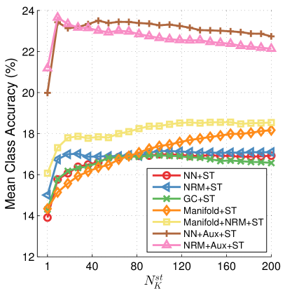
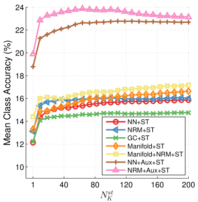
6 Conclusion

In this study, we investigated unsupervised word-vector embedding space representation for zero-shot action recognition for the first time. The fundamental challenge of zero-shot learning is the disjoint training and testing classes, and associated domain-shift. We explored the impact of four simple but effective strategies to address this: data augmentation, manifold regularization, self-training and hubness correction. Overall we demonstrated that given auxiliary and transductive access to testing data these strategies are complementary, and together facilitate a highly effective system that is even competitive against existing attribute-based approaches. If manually labelled attributes are available, our transductive strategies can produce the state-of-the-art performance. Moreover, our model has a closed-form solution that is very simple to implement (a few lines of matlab) and runs very efficiently. Finally, we also provide a unique analysis of the inter-class affinity for ZSL, giving insight into why and when ZSL works. This provides for the first time two new capabilities: the ability to predict the efficacy of a given ZSL scenario in advance, and a mechanism to guide the construction of suitable training sets for a desired set of target classes.

We have done some preliminary investigation of recognising novel classes when testing instances also include those of known training classes – a setting which is practically valuable but little studied. Designing algorithms specifically to deal with this challenging setting has received limited attention (Socher et al, 2013), and is still an open question. Another issue which is not fully addressed in this work is transferability prediction. Given limited labelling ability, it is desirable to annotate most useful training data to support zero-shot recognition. We discussed one possible way – measuring the semantic relatedness between candidate training class and testing classes. However the relation could be more complicated than pairwise, and the inclusion of a new training class could affect recognition of unknown classes in together with other training classes. How to best utilise labelling effort to support zero-shot recognition remains an open question.

References

- Aggarwal and Ryoo (2011) Aggarwal J, Ryoo M (2011) Human activity analysis: A review. ACM Computer Survey
- Akata et al (2015) Akata Z, Reed S, Walter D, Lee H, Schiele B (2015) Evaluation of output embeddings for fine-grained image classification. In: CVPR
- Belkin et al (2006) Belkin M, Niyogi P, Sindhwani V (2006) Manifold regularization: A geometric framework for learning from labeled and unlabeled examples. The Journal of Machine Learning Research
- Blank et al (2005) Blank M, Gorelick L, Shechtman E, Irani M, Basri R (2005) Actions as space-time shapes. In: ICCV
- Chen et al (2014) Chen J, Cui Y, Ye G, Liu D, Chang SF (2014) Event-driven semantic concept discovery by exploiting weakly tagged internet images. In: ICMR
- Deng et al (2009) Deng J, Dong W, Socher R, Li L, Li K, Li F (2009) Imagenet: A large-scale hierarchical image database. In: CVPR
- Dinu et al (2015) Dinu G, Lazaridou A, Baroni M (2015) Improving zero-shot learning by mitigating the hubness problem. In: ICLR, Workshop Track
- Frome et al (2013) Frome A, Corrado GS, Shlens J (2013) Devise: A deep visual-semantic embedding model. In: NIPS
- Fu et al (2012) Fu Y, Hospedales TM, Xiang T, Gong S (2012) Attribute learning for understanding unstructured social activity. In: ECCV
- Fu et al (2014a) Fu Y, Hospedales TM, Xiang T, Fu Z, Gong S (2014a) Transductive multi-view embedding for zero-shot recognition and annotation. In: ECCV
- Fu et al (2014b) Fu Y, Hospedales TM, Xiang T, Gong S (2014b) Learning multimodal latent attributes. IEEE Transactions on Pattern Analysis and Machine Intelligence
- Fu et al (2014c) Fu Y, Yang Y, Gong S (2014c) Transductive Multi-label Zero-shot Learning. In: BMVC
- Fu et al (2015a) Fu Y, Hospedales TM, Xiang T, Gong S (2015a) Transductive Multi-view Zero-Shot Learning. IEEE Transactions on Pattern Analysis and Machine Intelligence
- Fu et al (2015b) Fu Z, Xiang T, Kodirov E, Gong S (2015b) Zero-shot object recognition by semantic manifold distance. In: CVPR
- Gan et al (2015) Gan C, Lin M, Yang Y, Zhuang Y, GHauptmann A (2015) Exploring semantic inter-class relationships (sir) for zero-shot action recognition. In: AAAI
- Habibian et al (2014a) Habibian A, Mensink T, Snoek CG (2014a) Composite concept discovery for zero-shot video event detection. In: ICMR
- Habibian et al (2014b) Habibian A, Mensink T, Snoek CGM (2014b) VideoStory: A New Multimedia Embedding for Few-Example Recognition and Translation of Events. In: ACM Multimedia
- Jain and Snoek (2015) Jain M, Snoek CGM (2015) What do 15 , 000 object categories tell us about classifying and localizing actions ? In: CVPR
- Jain et al (2015) Jain M, van Gemert JC, Mensink T, Snoek CGM (2015) Objects2action: Classifying and localizing actions without any video example. In: ICCV
- Jiang et al (2015) Jiang Y, Wu Z, Wang J, Xue X, Chang S (2015) Exploiting feature and class relationships in video categorization with regularized deep neural networks. arXiv preprint arXiv:150207209
- Jiang et al (2011) Jiang YG, Ye G, Chang SF, Ellis DPW, Loui AC (2011) Consumer video understanding: a benchmark database and an evaluation of human and machine performance. In: ICMR
- Jiang et al (2013) Jiang YG, Liu J, Roshan Zamir A, Laptev I, Piccardi M, Shah M, Sukthankar R (2013) THUMOS challenge: Action recognition with a large number of classes
- Klaser et al (2008) Klaser A, Marszałek M, Schmid C (2008) A spatio-temporal descriptor based on 3d-gradients. In: BMVC
- Kodirov et al (2015) Kodirov E, Xiang T, Fu Z, Gong S (2015) Unsupervised Domain Adaptation for Zero-Shot Learning. In: ICCV
- Kuehne et al (2011) Kuehne H, Jhuang H, Garrote E, Poggio T, Serre T (2011) Hmdb: A large video database for human motion recognition. In: ICCV
- Lampert et al (2009) Lampert CH, Nickisch H, Harmeling S (2009) Learning to detect unseen object classes by between-class attribute transfer. In: CVPR
- Lampert et al (2014) Lampert CH, Nickisch H, Harmeling S (2014) Attribute-based classification for zero-shot visual object categorization. IEEE Transactions on Pattern Analysis and Machine Intelligence
- Laptev (2005) Laptev I (2005) On space-time interest points. International Journal of Computer Vision
- Larochelle et al (2008) Larochelle H, Erhan D, Bengio Y (2008) Zero-data learning of new tasks. In: AAAI
- Lazaridou et al (2014) Lazaridou A, Bruni E, Baroni M (2014) Is this a wampimuk? cross-modal mapping between distributional semantics and the visual world. In: ACL
- Liu et al (2011) Liu J, Kuipers B, Savarese S (2011) Recognizing human actions by attributes. In: CVPR
- Maaten and Hinton (2008) Maaten LVD, Hinton G (2008) Visualizing data using t-SNE. Journal of Machine Learning Research
- Marszalek et al (2009) Marszalek M, Laptev I, Schmid C (2009) Actions in context. In: CVPR
- Mensink et al (2014) Mensink T, Gavves E, Snoek CG (2014) Costa: Co-occurrence statistics for zero-shot classification. In: CVPR
- Mikolov et al (2013) Mikolov T, Sutskever I, Chen K (2013) Distributed representations of words and phrases and their compositionality. In: NIPS
- Milajevs et al (2014) Milajevs D, Kartsaklis D, Sadrzadeh M, Purver M (2014) Evaluating neural word representations in tensor-based compositional settings. In: EMNLP
- Mitchell and Lapata (2008) Mitchell J, Lapata M (2008) Vector-based Models of Semantic Composition. Computational Linguistics
- Niebles (2010) Niebles CWFFL Juan Carlos Chen (2010) Modeling temporal structure of decomposable motion segments for activity classification. In: ECCV
- Norouzi et al (2014) Norouzi M, Mikolov T, Bengio S, Singer Y, Shlens J, Frome A, Corrado GS, Dean J (2014) Zero-shot learning by convex combination of semantic embeddings. In: ICLR
- Over et al (2014) Over P, Fiscus J, Sanders G, Joy D, Michel M, Smeaton-Alan AF, Quénot-Georges G (2014) Trecvid 2013–an overview of the goals, tasks, data, evaluation mechanisms, and metrics
- Palatucci et al (2009) Palatucci M, Hinton G, Pomerleau D, Mitchell TM (2009) Zero-shot learning with semantic output codes. In: NIPS
- Pan and Yang (2010) Pan SJ, Yang Q (2010) A survey on transfer learning. IEEE Transactions on Knowledge and Data Engineering
- Perronnin et al (2010) Perronnin F, Sánchez J, Mensink T (2010) Improving the fisher kernel for large-scale image classification. In: ECCV
- Poppe (2010) Poppe R (2010) A survey on vision-based human action recognition. Image and vision computing
- Rohrbach et al (2010) Rohrbach M, Stark M, Szarvas G, Gurevych I, Schiele B (2010) What helps where - and why? Semantic relatedness for knowledge transfer. In: CVPR
- Rohrbach et al (2011) Rohrbach M, Stark M, Schiele B (2011) Evaluating knowledge transfer and zero-shot learning in a large-scale setting. In: CVPR
- Rohrbach et al (2013) Rohrbach M, Ebert S, Schiele B (2013) Transfer learning in a transductive setting. In: NIPS
- Rohrbach et al (2016) Rohrbach M, Rohrbach A, Regneri M, Amin S, Andriluka M, Pinkal M, Schiele B (2016) Recognizing fine-grained and composite activities using hand-centric features and script data. IJCV
- Romera-Paredes and Torr (2015) Romera-Paredes B, Torr PHS (2015) An embarrassingly simple approach to zero-shot learning. In: ICML
- Scholkopf and Smola (2002) Scholkopf B, Smola AJ (2002) Learning with Kernels: Support Vector Machines, Regularization, Optimization, and Beyond. MIT Press. (2002),
- Schuldt et al (2004) Schuldt C, Laptev I, Caputo B (2004) Recognizing human actions: A local svm approach. In: ICPR
- Scovanner et al (2007) Scovanner P, Ali S, Shah M (2007) A 3-dimensional sift descriptor and its application to action recognition. In: ACM Multimedia
- Shao et al (2015) Shao L, Zhu F, Li X (2015) Transfer learning for visual categorization: a survey. IEEE transactions on neural networks and learning systems
- Socher et al (2013) Socher R, Ganjoo M, Manning CD, Ng AY (2013) Zero-shot learning through cross-modal transfer. In: NIPS
- Soomro et al (2012) Soomro K, Zamir AR, Shah M (2012) Ucf101: A dataset of 101 human actions classes from videos in the wild. arXiv preprint arXiv:12120402
- Wang and Schmid (2013) Wang H, Schmid C (2013) Action Recognition with Improved Trajectories. In: ICCV
- Wang et al (2013) Wang H, Kläser A, Schmid C, Liu CL (2013) Dense trajectories and motion boundary descriptors for action recognition. International Journal of Computer Vision
- Wang et al (2015) Wang H, Oneata D, Verbeek J, Schmid C (2015) A robust and efficient video representation for action recognition. International Journal of Computer Vision
- Wu et al (2014) Wu S, Bondugula S, Luisier F, Zhuang X, Natarajan P (2014) Zero-Shot Event Detection Using Multi-modal Fusion of Weakly Supervised Concepts. In: CVPR
- Xu et al (2015) Xu X, Hospedales T, Gong S (2015) Semantic embedding space for zero shot action recognition. In: ICIP
- Yang and Hospedales (2015) Yang Y, Hospedales T (2015) A unified perspective on multi-domain and multi-task learning. In: ICLR
- Yeffet and Wolf (2009) Yeffet L, Wolf L (2009) Local trinary patterns for human action recognition. In: ICCV
- Zhao et al (2013) Zhao F, Huang Y, Wang L, Tan T (2013) Relevance topic model for unstructured social group activity recognition. In: NIPS
- Zheng and Jiang (2014) Zheng J, Jiang Z (2014) Submodular Attribute Selection for Action Recognition in Video. In: NIPS
- Zhou et al (2004) Zhou D, Bousquet O, Weston J (2004) Learning with local and global consistency. In: NIPS