Dark Energy Parametrization motivated by Scalar Field Dynamics

Abstract

We propose a new Dark Energy parametrization based on the dynamics of a scalar field. We use an equation of state $w=(x-1)/(x+1)$, with $x=E_{k}/V$, the ratio of kinetic energy $E_{k}=\dot{\phi}^{2}/2$ and potential $V$. The eq. of motion gives $x=(L/6)(V/3H^{2})$ and has a solution $x=([(1+y)^{2}+2L/3]^{1/2}-(1+y))/2$ where $y\equiv\rho_{m}/V$ and $L\equiv(V^{\prime}/V)^{2}(1+q)^{2},\,q\equiv\ddot{\phi}/V^{\prime}$. The resulting EoS is $w=\left(6+L-6\sqrt{(1+y)^{2}+2L/3}\right)/\left(L+6y\right)$. Since the universe is accelerating at present time we use the slow roll approximation in which case we have $|q|\ll 1$ and $L\simeq(V^{\prime}/V)^{2}$. However, the derivation of $w$ is exact and has no approximation. By choosing an appropriate ansatz for $L$ we obtain a wide class of behavior for the evolution of Dark Energy without the need to specify the potential $V$. The EoS $w$ can either grow and later decrease, or other way around, as a function of redshift and it is constraint between $-1\leq w\leq 1$ as for any canonical scalar field with only gravitational interaction. To determine the dynamics of Dark Energy we calculate the background evolution and its perturbations, since they are important to discriminate between different DE models. Our parametrization follows closely the dynamics of a scalar field scalar fields and the function $L$ allow us to connect it with the potential $V(\phi)$ of the scalar field $\phi$.

I Introduction

In the last years the study of our universe has received a great deal of attention since on the one hand fundamental theoretical questions remain unanswered and on the other hand we have now the opportunity to measure the cosmological parameters with an extraordinary precision. Existing observational experiments involve measurement on CMB planck ; wmap9 or large scale structure ”LSS” LSS or supernovae SNIa SN , and new proposals are carried out new .

Taking a flat universe dominated at present time by matter and Dark Energy ”DE”, and using a constant equation of state $w$ for DE, one finds $\Omega_{\rm DE}\simeq 0.714\pm 0.012$, $\Omega_{\rm m}\simeq 0.286\pm 0.012$ with $w=-1.037^{+0.071}_{-0.070}$ from WMAP9 results wmap9 and $\Omega_{\rm DE}\simeq 0.6914^{+0.019}_{-0.021}$, $\Omega_{\rm m}\simeq 0.208^{+0.019}_{-0.021}$ with $w=-1.13^{+0.13}_{-0.14}$ from Planck planck , SNLS SN and BAO LSS measurements. The constraint on curvature is $-0.0013<\Omega_{k}<0.0028$ for WMAP9 wmap9 and $|\Omega_{k}|=0.0005$ for Planck planck using a ${\rm\Lambda CDM}$ model, i.e. $w=-1$ for DE. At present time, the equation of state ”EoS” of DE depends on the priors, choice of parameters and on the data used for the analysis as can be seen from the results obtained by either WMAP or Planck collaboration groups planck ; wmap9 . A more precise determination of the EoS of DE will be carried out in new which together with precise measurements of CMB such as planck ; wmap9 will yield a better understanding of the dynamics of Dark Energy. With better data we should be able to study in more detail the nature of Dark Energy, a topic of major interest in the field DE.rev . Since the properties of Dark Energy are still under investigation, different DE parametrization have been proposed to help discern on the dynamics of DE DEparam -quint.ax . Some of these DE parametrization have the advantage of having a reduced number of parameters, but they may lack a physical motivation and may also be too restrictive. The evolution of DE background may not be enough to distinguish between different DE models and therefore the perturbations of DE may be fundamental to differentiate between them.

Perhaps the best physically motivated candidates for Dark Energy are scalar fields, which can interact only via gravity SF.Peebles ; tracker ; quint.ax or interact weakly with other fluids, e.g. Interacting Dark Energy ”IDE” modelsIDE ; IDE.ax . In this work we will concentrate on canonically normalized scalar fields minimally coupled to gravity. Scalar fields have been widely studied in the literature SF.Peebles ; tracker ; quint.ax and special interest was devoted to tracker fields tracker , since in this case the behavior of the scalar field $\phi$ is weakly dependent on the initial conditions set at an early epoch, well before matter-radiation equality. In this class of models a fundamental question is why DE is relevant now, also called the coincidence problem, and this can be understand by the insensitivity of the late time dynamics on the initial conditions of $\phi$. However, tracker fields may not give the correct phenomenology since the have a large value of $w$ at present time. We are more interested at this stage to work from present day redshift $z=0$ to larger values of $z$, in the region where DE and its perturbations are most relevant. Interesting models for DE and DM have been proposed using gauge groups, similar to QCD in particle physics, and have been studied to understand the nature of Dark Energy GDE.ax and also Dark Matter GDM.ax .

Here we propose a new DE parametrization based on scalar fields dynamics, but the parametrization of $w$ can be used without the connection to scalar fields. This parametrization has a rich structure that allows $w$ to have different evolutions, it may grow and later decrease or other way around. We also determine the perturbations of DE which together with the evolution of the homogenous part can single out the nature of DE. With the underlying connection between the evolution of $w$ and the dynamics of scalar field we could determine the potential $V(\phi)$. The same motivation of parameterizing the evolution of scalar field was presented in an interesting paper huang . We share the same motivation but we follow a different path. We have the same number of parameters but a richer structure and it is easier to obtain information of the scalar potential $V(\phi)$ .

We organize the work as follows: in Sec.I.1 we give a brief overview of our DE parametrization. In Sec.II we present the scalar field and we define the variables used in this work. In Sec.III we present the dynamics of a scalar field and the set up for our DE parametrization given in Sec.IV. We calculate the DE perturbations in Sec.V and finally we conclude in Sec.VI.

I.1 Overview

We present here an overview of our $w$ parametrization. The EoS is

$$w=\frac{p}{\rho}=\frac{x-1}{x+1}.$$ (1)

with $x\equiv E_{k}/V$ the ratio of kinetic energy $E_{k}=\dot{\phi}^{2}/2$ and potential $V(\phi)$. This corresponds to a canonically normalized scalar field. The equation of motion of the scalar field gives (c.f. eq.(21)),

$$x=\frac{\left(\sqrt{1+\frac{2L}{3(1+y)^{2}}}-1\right)\left(1+y\right)}{2},$$ (2)

where $y\equiv\rho_{m}/V$ the ratio of matter density and $V$, $L\equiv(V^{\prime}/V)^{2}A$ with $A\equiv(1+q)^{2},q\equiv\ddot{\phi}/V^{\prime}$. Eq.(2) is an exact equation and is valid for any fluid evolution and/or for an arbitrary potential $V(\phi)$. In terms of $L$ and $y$ the EoS is

$$w=\frac{6+L-6\sqrt{(1+y)^{2}+2L/3}}{L+6y}=-1+\frac{6(1+y)-6\sqrt{(1+y)^{2}+2L/3}}{L+6y}$$ (3)

which we consider our master equation and it is valid for any value of $L$ and $y$ and not only in the slow roll regime.

The aim of our proposed parametrization for $L,y$ is to cover a wide range of DE behavior. Of course other interesting parameterizations are possible. The dynamics of scalar fields with canonical kinetic terms has an EoS constrained between $-1<w<1$ and gives an accelerating universe only if $\lambda=-V^{\prime}/V\rightarrow 0$ or to a constant $|\lambda|<1$ with $w=-1+\lambda^{2}/3$ quint.ax (for an EoS $w<-0.8$ one needs $\lambda<0.8$). From the dynamics of scalar fields we know that the evolution of $w$ close to present time is model dependent. For example, in the case of $V=V_{o}\phi^{-2/3}$, used as a model of DE derived from gauge theory GDE.ax , the shape of $w(z)$ close to present time depends on the initial conditions and it may grow or decrease as a function of redshift $z$. We also know that tracker fields are attractor solutions but in most cases they do not give a negative enough $w_{o}$ tracker . In this class of models the EoS, regardless of its initial value, goes to a period of kinetic domination where $w\simeq 1$ and later has a steep transition to $w\simeq-1$, which may be close to present time, and finally it grows to $w_{o}$ in a very model and initial condition dependent way. Furthermore, if instead of having a single potential term we have two competing terms close to present time, the evolution of $w(z)$ would even be more complicated. Therefore, instead of deriving the potential $V$ from theoretical models as in GDE.ax we propose to use an ansatz for the functions $L$ and $y$ which on one hand should cover a wide range of DE behavior with the least number of parameters but without sacrificing generality, and on the other hand we would like to have this ansatz as close as possible to the known scalar field dynamics. We believe that using our model will greatly simplify the extraction of DE dynamics from the future observational data. We propose therefore the ansatz (c.f. eqs.(75) and (77) )

$$L= L_{o}+L_{1}y^{\xi}f(z)$$ (4)

$$f(z)= \frac{(z/zt)^{k}}{1+(z/z_{t})^{k}}$$ (5)

where $y=y_{o}a^{3w_{o}}$ and $L_{o},L_{1}$ are free parameters giving $w_{o}$ at present time (a subscript $o$ represents present time quantities) and $w_{i}=w(z\gg z_{t})$ at early times, $f(z)$ is a function that goes from $f(z=0)=0$ at $z=0$ to $f(z\gg 1)=1$ at large $z$. The parameter $z_{t}$ sets the transition redshift between $w_{o}$ and $w_{i}$ while $k$ sets the steepness of the transition and $\xi$ takes only two values $\xi=1$ or $\xi=0$ (see sect.(IV)).

Since the universe is accelerating at present time we may take the slow roll approximation where $|q|\ll 1,A\simeq 1$ and $L\simeq(V^{\prime}/V)^{2}$. In this case one has $w\simeq-1+L/3(1+y)$. However, the derivation of $L$ in eq.(2) is exact and has no approximation. We will show in section IV that $w$ can have a wide range of behavior and in particular $w$ can decrease and later increase as a function of redshift and vice versa, therefore the shape and steepness are not predetermined by the choice of our parametrization. Of course we could use other parametrizations for $L$ since the evolution of $x$ and $w$ in eqs.(1) and (2) are fully valid. There is also no need to have any reference to the underlying scalar field dynamics, i.e. our parametrization is not constrained to scalar field dynamics. However, it is when we interpret $x,L$ and $y$ as: $x\equiv\dot{\phi}^{2}/2V$, $L=(V^{\prime}/V)^{2}A$ and $y=\rho_{m}/V$, that we connect the evolution of $w$ to the scalar potential $V(\phi)$.

Finally DE perturbations are important in distinguishing between different DE models hu -DE.p and we will show that a steep transition of $w$ has a bump in the adiabatic sound speed $c_{a}^{2}$ which could be detected in large scale structure DE.p.sf ; DE.p . At an epoch where the universe is dominated by DM and DE the total perturbation $\delta_{T}=\delta\rho_{T}/\rho_{T}=\Omega_{\rm DM}\delta\rho_{DM}+\Omega_{\rm DE}\delta\rho_{DE}$ and if $\Omega_{\rm DE}$ is not much smaller than $\Omega_{\rm DM}$, i.e. for low redshift $z$, then the evolution of $\delta\rho_{DE}$ may have an important contribution to $\delta_{T}$, as discussed in Sec.V.

II Scalar Field Dynamics

We are interested in obtaining a new DE parametrization inferred from scalar fields SF.Peebles -IDE.ax . Since it is derived from the dynamics of a scalar field $\phi$ we can also determine its perturbations which are relevant in large scale structure formation. We start with a FRW metric with a line element

$$ds^{2}=dt^{2}-a(t)^{2}\left(\frac{dr^{2}}{1-kr^{2}}+r^{2}d\theta^{2}+r^{2}\sin(\theta)d\varphi^{2}\right)$$ (6)

and a canonically normalized scalar field $\phi(t,x)$ with a potential $V(\phi)$ and minimally coupled to gravity. The homogenous part of $\phi$ has an equation of motion

$$\ddot{\phi}+3H\dot{\phi}+V^{\prime}(\phi)=0$$ (7)

where $V^{\prime}\equiv dV/d\phi$, $H=\dot{a}/a$ is the Hubble constant, $a(t)$ is the scale factor and a dot represents derivative with respect to time $t$. Since we are interested in the epoch for small redshift z, with $a_{o}/a=1+z$, we only need to consider matter and DE and we have

$$3H^{2}=\rho_{m}+\rho_{\phi},$$ (8)

in natural units $8\pi G=1,c=\hbar=1$. The energy density $\rho$ and pressure $p$ for the scalar field are

$$\rho_{\phi}=\frac{1}{2}\dot{\phi}^{2}+V,\;\;\;p_{\phi}=\frac{1}{2}\dot{\phi}^{2}-V.$$ (9)

We define the ratio of kinetic energy and potential energy as

$$x\equiv\frac{\dot{\phi}^{2}}{2V}$$ (10)

and the equation of state parameter ”EoS” becomes

$$w\equiv\frac{p_{\phi}}{\rho_{\phi}}=\frac{\dot{\phi}^{2}/2-V}{\dot{\phi}^{2}/2+V}=\frac{x-1}{x+1}$$ (11)

or

$$w=-1+\delta w,\;\;\;\;\;\;\delta w\equiv\frac{2x}{1+x}.$$ (12)

The value of $x$ determines $w$ or inverting eq.(11) we have $x=(1+w)/(1-w)$. Since $x\geq 0$ the Dark Energy EoS $w$ is in the range $-1\leq w\leq 1$. For growing $x$ the EoS $w$ becomes larger and at $x\gg 1$ one has $w\simeq 1$ while a decreasing $x$ has $w\rightarrow-1$ for $x\rightarrow 0$. In terms of $x$ we have

$$\rho_{\phi}=V(x+1),\;\;p_{\phi}=V(x-1),\;\;\rho_{m}=Vy$$ (13)

where we defined the ratio of and scalar potential $V$ as

$$y\equiv\frac{\rho_{m}}{V}.$$ (14)

Finally we can express $\Omega_{\phi},\Omega_{m}$ and $H$ in terms of $x,y$ and $V$ as

$$\Omega_{\phi} = \frac{1+x}{1+x+y},\;\;\;\;\Omega_{m}=\frac{y}{1+x+y},$$ (15)

$$3H^{2} = \rho_{m}+\rho_{\phi}=V(1+x+y).$$ (16)

The equation of motion for $\phi$ is

$$\dot{\phi}=-\frac{V^{\prime}+\ddot{\phi}}{3H}=-\frac{V^{\prime}(1+q)}{3H}$$ (17)

and we can write

$$x\equiv\frac{\dot{\phi}^{2}}{2V}=\frac{V}{3H^{2}}\frac{V^{\prime 2}}{6V^{2}}\left(1+q\right)^{2}=\frac{V}{3H^{2}}\frac{L}{6}$$ (18)

with

$$L\equiv \left(\frac{V^{\prime}}{V}\right)^{2}(1+q)^{2}=\lambda^{2}A,$$ (19)

$$\lambda\equiv -\frac{V^{\prime}}{V},\;\;\;\;\;\;q\equiv\frac{\ddot{\phi}}{V^{\prime}},\;\;\;\;\;\;\;A\equiv\left(1+q\right)^{2}.$$

Since the r.h.s. of eq.(18) still depends on $x$ through $H$ we use eq.(16) and eq.(18) becomes then

$$x=\frac{L}{6(1+x+y)}$$ (20)

which has a simple solution

$$x=\frac{\left(\sqrt{1+\frac{2L}{3(1+y)^{2}}}-1\right)\left(1+y\right)}{2}=\frac{\sqrt{(1+y)^{2}+2L/3}-(1+y)}{2}.$$ (21)

Substituting eq.(21) into eq.(11) we obtain our DE parametrization as a function of $L$ and $y$

$$w=\frac{\sqrt{(1+y)^{2}+2L/3}-(3+y)}{\sqrt{(1+y)^{2}+2L/3}+(1+y)}.$$ (22)

If we multiply in eq.(22) the numerator and denominator by $\sqrt{(1+y)^{2}+2L/3}-(1+y)$ we obtain an alternative and useful expression for the EoS

$$w=\frac{6+L-6\sqrt{(1+y)^{2}+2L/3}}{L+6y}=-1+\frac{6(1+y)-6\sqrt{(1+y)^{2}+2L/3}}{L+6y}$$ (23)

and

$$\delta w=w+1=\frac{6(1+y)-6\sqrt{(1+y)^{2}+2L/3}}{L+6y}$$ (24)

which we consider our master expression for $w$. It is a relatively simple expression but more important is that eqs.(22) and (23) are exact and therefore valid for any values of $L$ and $y$ and not only at a slow roll regime. We will see in the next section some physically motivated limits of eq.(23). Finally, inverting the expression of $w$ we can obtain $L$ as a function of $w$ and $y$

$$L=\frac{12(1+w)+6y(1-w^{2})}{(1-w)^{2}}$$ (25)

and $y$ as a function of $w$ and $L$

$$y=\frac{L(1-w)^{2}-12(1+w)}{6(1-w^{2})}.$$ (26)

II.0.1 Dynamics and Limits for $L,x,w$

Using eq.(20) we can express

$$w=-1+\delta w=-1+\frac{2L}{L+6(1+x+y)},$$ (27)

and it is an exact equation, however $x$ depends on $y,L$ through eq.(21). If we take $x<(1+y)$, valid in the slow roll approximation, one has for arbitrary values of $y$ and $L$

$$x=\frac{L}{6(1+y)},\;\;\;w=-1+\frac{L}{3(1+y)}$$ (28)

and as $L\rightarrow 0$ we have $x\rightarrow 0$ and $w\rightarrow-1$. Notice that

$$y=\frac{\rho_{m}}{V}=\frac{\rho_{m}}{\rho_{\phi}}\frac{2}{(1-w)}=\frac{\Omega_{m}}{\Omega_{\phi}}\frac{2}{(1-w)}$$ (29)

and we then expect that $y$ increases as a function of redshift z when matter dominates over Dark Energy and with $y_{o}=y(a_{o})\simeq 0.25$ at present time. We expect then that $x<(1+y)$ will be satisfied beyond the slow roll approximation and eq.(28) is valid for a wide range of the parameter’s values.

If we take $L\gg 1$ with $y$ constant in eq.(23) we get the limit

$$x=\sqrt{\frac{L}{6}},\;\;\;w=1-2\sqrt{\frac{6}{L}}$$ (30)

and for $L/y\rightarrow L_{1}$ constant with $y\gg 1,L\gg 1$ we have $x$ and $w$ also constants given by

$$x=\frac{L_{1}}{6},\;\;\;w=\frac{L_{1}-6}{L_{1}+6}=-1+\frac{2L_{1}}{6+L_{1}}.$$ (31)

Clearly depending on the value of $L$ we can have a decreasing or increasing $x$ and $w$ as a function of redshift. For example for $w=0$ one has $L_{1}=6$ while for $w=1/3$ one requires $L_{1}=12$ at large $y$.

Since $w$ is only a function of $x$ we have $dw=w_{x}dx$ or as a function of redshift

$$w_{z}=w_{x}x_{z}$$ (32)

with

$$w_{x}=\frac{2}{(1+x)^{2}}\geq 0.$$ (33)

The sign of $w_{z}$ depends then only on the sign of $x_{z}$ given by

$$x_{z}=x_{y}y_{z}+x_{L}L_{z}$$ (34)

with

$$x_{y}=-\frac{x}{1+2x+y},\;\;x_{L}=\frac{1}{6(1+2x+y)}.$$ (35)

Clearly $x_{L}$ is positive definite while $x_{y}\leq 0$. In general we can assume that DE redshifts slower than matter, at least for small z , since DE has $w<0$ and matter $w_{m}=0$, so $y=\rho_{m}/V$ is a growing function of z, i.e. $y_{z}>0$ and $x_{y}y_{z}\leq 0$. Therefore if $L_{z}$ is negative we have $x_{L}L_{z}<0$ and a decreasing $x$ and $w$ as a function of redshift. However, if $L_{z}$ is positive then the sign of $x_{L}L_{z}$ is positive and $w$ may grow or decrease depending on the magnitude of $|x_{y}y_{z}|$ compared to $|x_{L}L_{z}|$.

II.0.2 Slow Roll Approximation

The evolution of $x$ as a function of $L$ and $y$ is given in eq.(21) and here we will show some phenomenological interesting limits. Since the field $\phi$ should be responsible for accelerating the universe we know that $w$ must be close to $-1$ at present time, and the field $\phi$ must satisfy the slow roll approximation. In the slow roll approximation one has $|\ddot{\phi}|\ll|3H\dot{\phi}|\simeq|-V^{\prime}|$ and we then have

$$|q\equiv\frac{\ddot{\phi}}{V^{\prime}}|=|\frac{3H\dot{\phi}}{V^{\prime}}-1|\ll 1$$ (36)

with $A\simeq 1$ and the function $L$ becomes

$$L\simeq\left(\frac{V^{\prime}}{V}\right)^{2}=\lambda^{2}.$$ (37)

We name a full slow roll approximation when $\ddot{\phi}=0$ (i.e. $3H\dot{\phi}=-V^{\prime}$ and $q=0$). This full slow roll approximation is more suitable in inflation where one has a long period of inflation, however Dark Energy does dominate only recently and so we do not expect this approximation to hold for a long period of time and should not be taken as a working hypothesis for DE parametrization.

II.0.3 Late time attractor Solution

The evolution of scalar fields has been studied in quint.ax and a late time attractor for an accelerating universe requires $w<-1/3,\lambda^{2}<2$ with $\Omega_{\phi}\rightarrow 1$. In the limit $\lambda^{2}<3$ with $\rho_{m}\ll\rho_{\phi}$ one has

$$\frac{\dot{\phi}^{2}}{6H^{2}}=\frac{\lambda^{2}}{6},\;\;\;\;\;\;\frac{V}{3H^{2}}=1-\frac{\lambda^{2}}{6}$$ (38)

giving

$$x\equiv\frac{\dot{\phi}^{2}}{2V}=\frac{\lambda^{2}}{6-\lambda^{2}},\;\;\;\;\;\;w=-1+\frac{\lambda^{2}}{3}.$$ (39)

Notice that eq.(28) reduces to eq.(39) in the limit $y\ll 1$ with $L\simeq\lambda^{2}$, and therefore eq.(28) generalizes eq.(39). For large redhsift z we expect $y$ to increase and eq.(39) would not longer be valid and we should take instead eq.(28).

III Dynamical Evolution

Differentiating $x$ and $y$ w.r.t. time or equivalently as a function $N\equiv\rm ln[a]$, where $a$ is the scale factor, we get the evolution of $x$ and $y$. Using the definition of $x$ in eq.(18), $\dot{\rho}_{m}=-3H\rho_{m}$, $\ddot{\phi}=-3H\dot{\phi}-V^{\prime}$ and $f_{N}\equiv df/dN=\dot{f}/H$ for any function $f[N(t)]$, we get

$$\dot{x}=\frac{\dot{\phi}}{V}\left(\ddot{\phi}-xV^{\prime}\right)=\frac{\dot{\phi}V^{\prime}}{V}\left(q-x\right)=6Hx\left(\frac{x-q}{1+q}\right)$$ (40)

$$x_{N}=\frac{\dot{x}}{H}=6x\left(\frac{x-q}{1+q}\right)=6x\left(\frac{1+x}{1+q}-1\right)$$ (41)

and $\dot{y}=Hy_{N}$ with

$$y_{N}=\frac{\dot{y}}{H}=-3y-\frac{yV^{\prime}\dot{\phi}}{HV}=-3y\left(1-\frac{2x}{1+q}\right).$$ (42)

We see that eqs.(41) and (42) are uniquely determined by a single function $q\equiv\ddot{\phi}/V^{\prime}$. The critical points for $\dot{x}=0$, i.e. $\dot{\phi}=0$, have $x=0$ or $x=q$ while $\dot{y}=0$ is satisfied for $y=0$ and $2x=1+q$. The case, $\dot{\phi}=x=0$ has $w=-1$ and $\dot{y}=-3Hy$ which gives a solution $y=y_{i}(a/a_{i})^{-3}$, a constant $V(\phi)$ and the limits $\Omega_{\phi}\rightarrow 1,y\rightarrow 0$ and $\Omega_{m}\rightarrow 0$. In the case $q=x$ the EoS becomes $w=(q-1)/(q+1)$ and it will take different constant values. Setting $q=x$ constant in eq.(42) we get $\dot{y}=3Hyw$ with $w$ constant one has a solution

$$y=y_{o}\left(\frac{a}{a_{o}}\right)^{3w}.$$ (43)

For $q=x<1$ we have $w<0$, $y\rightarrow 0$ and $\Omega_{\phi}\rightarrow 1$. Finally, we can satisfy $\dot{x}=\dot{y}=0$ for $x=y=0$ or $x=q=1$ giving $w=0$ and $y$ constant (c.f. eq.(43)).

Therefore, having an increasing or decreasing $x$ depends on the sign of $\dot{\phi}(\ddot{\phi}-xV^{\prime})=\dot{V}(q-x)$ and it can vary as a function on time depending on the values of $x$ and $q$, i.e. on the choice of the potential $V(\phi)$. If we take what we call a full slow roll defined by $\ddot{\phi}=q=0$ and $3H\dot{\phi}=-V^{\prime}$ then eq.(41) becomes

$$\dot{x}=6Hx^{2}$$ (44)

which is positive definite, i.e. $\dot{x}\geq 0$. Using $H=\dot{a}/a$ we can express eq.(44) giving a solution

$$x=\frac{x_{o}}{1+6x_{o}Ln(a_{o}/a)}=\frac{x_{o}}{1+6x_{o}Ln(1+z)}.$$ (45)

Therefore if the condition $q=0$ or $|q=\ddot{\phi}/V^{\prime}|\ll x$ is satisfied, then from eq.(45) we have a decreasing function for $x$ as a function of redshift z and therefore $w(z)$ also decreases. However, we do not expect the universe to be in a full slow roll regime and when $x$ is small, e.g. $w<-0.9$ one has $x<0.05$, the slow roll condition $|\ddot{\phi}|<|V^{\prime}|$ does not imply that $q=\ddot{\phi}/V^{\prime}\ll x$. Therefore, the sign of $\dot{x}$ can be positive or negative depending on the sign and size of $q=\ddot{\phi}/V^{\prime}$ compared to $x$ and $x$ can either grow or decrease. In the region where $q=\ddot{\phi}/V^{\prime}<x$ we have $\dot{x}>0$ while for $q=\ddot{\phi}/V^{\prime}>x$ we have $\dot{x}<0$. The value of $q$ parameterizes then the amount of slow roll of the potential and a full slow roll has $q=0$ but we expect to be only in an approximate slow roll regime with $|q|\ll 1$ and $L\simeq\lambda^{2}$. We discuss the dynamics of $q$ in section V. In the present work we do not want to study the critical points of the dynamical equations but the evolution of $x$ close to present time when the universe is accelerating with $x$ close to zero ($w$ close to -1) but not exactly zero with $\dot{\phi}\neq 0$ and $\ddot{\phi}\neq xV^{\prime}$

III.1 Dynamical evolution of $x$ and $y$

The dynamical eqs.(41) and (42) can also be written in terms of $V_{N}/V,\,V_{N}\equiv dV/dN$ as

$$x_{N} \equiv \frac{dx}{dN}=-\left(6x+(1+x)\frac{V_{N}}{V}\right)$$

$$y_{N} \equiv \frac{dy}{dN}=-y\left(3+\frac{V_{N}}{V}\right).$$ (46)

From eqs.(III.1) we clearly see that the behavior of $x$ and $y$ is completely determined by a single function $V_{N}/V$ and we define

$$\zeta\equiv-\frac{V_{N}}{V}=-\frac{V^{\prime}\phi_{N}}{V}=\lambda(\phi)\;\phi_{N}$$ (47)

with $\lambda=-V^{\prime}/V$. It is easy to see from eqs.(41), (42) and (III.1) that the function $\zeta$ is given in terms of $x$ and $q$ as

$$\zeta=-\frac{V_{N}}{V}=\frac{6x}{1+q}.$$ (48)

In the case where the scalar field rolls down its minimum we will have $\dot{V}=V^{\prime}\phi_{N}$ negative giving a $\zeta>0$. In the simple case of having $\zeta$ constant the solution to eqs.(III.1) are simply

$$x=x_{i}e^{-(6-\zeta)(N-N_{i})}+\left(\frac{\zeta}{6-\zeta}\right)\left(1-e^{-(6-\zeta)(N-N_{i})}\right)$$ (49)

and

$$y=y_{i}e^{-(3-\zeta)(N-N_{i})}$$ (50)

with initial conditions $x=x_{i},y=y_{i}$ at $N=N_{i}$. The asymptotic values of $x$ and $y$ depend on the value of $\zeta$. The critical points of the system in eqs.(III.1) give for $x_{N}=0$ a solution

$$\zeta=-\frac{V_{N}}{V}=\frac{6x}{1+x}$$ (51)

and if we invert eq.(51) we simply get

$$x=\frac{\zeta}{6-\zeta}$$ (52)

and an EoS

$$w=\frac{x-1}{x+1}=-1+\frac{\zeta}{3}.$$ (53)

Using eq.(53) we have $3-\zeta=-3w$ and eq.(50) becomes then

$$y=y_{i}e^{3w(N-N_{i})}=y_{i}\left(\frac{a}{a_{i}}\right)^{3w}$$ (54)

which is valid for $\zeta$ constant. We clearly see that the value of $\zeta$ determines the asymptotic behavior of $x,y$ and of the scalar field energy density $\rho_{\phi}$. If $\zeta<3$ the scalar field will dominate since $w<0$ and we will have $y\rightarrow 0,\Omega_{\phi}\rightarrow 1$ and $x=\zeta/(6-\zeta)<1$, while for $\zeta=3$ we have $x=1,w=0$ and $y$ constant given in eq.(59). Finally for $\zeta>3$ we get $x>1,w>0$ and $y\rightarrow\infty$ with $\Omega_{\phi}\rightarrow 0$. Of course an accelerated universe requires $w<0,x<1$ and therefore $\zeta<3$ close to present time. However, in general the value of $\zeta$ will be time (or $N$) dependent.

III.1.1 $\zeta$ as a function of $x$ and $y$

The function $\zeta$ is a function of $\phi$ and $\phi_{N}$, as we can see form eq.(47) and we can express $\phi_{N}$ in terms of $x,y$ as

$$\phi_{N}={\rm sign}[\dot{\phi}]\;\sqrt{\frac{6x}{1+x+y}}$$ (55)

(for a rolling scalar field $\dot{\phi}>0$ but we have kept the term ${\rm sign}[\dot{\phi}]$ for completeness),

$$\zeta=-\frac{V_{N}}{V}={\rm sign}[\dot{\phi}]\;\lambda\;\sqrt{\frac{6x}{1+x+y}}$$ (56)

and the eqs.(III.1) read now

$$x_{N}= -6x+{\rm sign}[\dot{\phi}]\;(1+x)\;\lambda\;\sqrt{\frac{6x}{1+x+y}}$$ (57)

$$y_{N}= -3y+{\rm sign}[\dot{\phi}]\;y\;\lambda\;\sqrt{\frac{6x}{1+x+y}}.$$ (58)

The amount of $\Omega_{\phi}$ can be determined at the critical point $x_{N}=y_{N}=0$ giving $x=1,w=0$ (i.e. the scalar field redshifts as the barotropic fluid which in our case is matter $w_{m}=0$) and

$$y =\left(\frac{\lambda^{2}}{\zeta}-1\right)\left(\frac{6}{6-\zeta}\right)=2\left(\frac{\lambda^{2}}{3}-1\right),$$ (59)

$$\Omega_{\phi} =\frac{\zeta}{\lambda^{2}}=\frac{3}{\lambda^{2}}.$$ (60)

This solution is valid for $\lambda^{2}>3$ and has a $\zeta=3$. The critical point for $\lambda^{2}<3$ has

$$x=\frac{\lambda^{2}}{6-\lambda^{2}},\;\;\;\;w=-1+\frac{\lambda^{2}}{3},\;\;\;\;y\rightarrow 0,\;\;\;\;\Omega_{\phi}\rightarrow 1.$$ (61)

III.2 Dynamical System for $\hat{x}\equiv\dot{\phi}/\sqrt{6}H$ and $\hat{y}\equiv\sqrt{V/3H}$

As a matter of completeness we present here also the dynamical evolution equations in term of the variables $\hat{x}\equiv\dot{\phi}/\sqrt{6}H=\phi_{N}/\sqrt{6}$ and $\hat{y}\equiv\sqrt{V/3H}$ which have been widely used in the literature for studying the dynamics of scalar fields quint.ax . In this case the dynamical equations are given by n

$$\hat{x}_{N} = -3\hat{x}+\sqrt{3\over 2}\lambda\,\hat{y}^{2}-\hat{x}\frac{H_{N}}{H}$$

$$\hat{y}_{N} = -\sqrt{3\over 2}\lambda\,\hat{x}\,\hat{y}-\hat{y}\frac{H_{N}}{H}$$ (62)

$$\frac{H_{N}}{H} = -{3\over 2}[1+\hat{x}^{2}-\hat{y}^{2}]$$

valid for a flat universe with a scalar field and matter. These equations depend only on the function $\lambda(\phi(N))=-V^{\prime}/V$. The variables $x,y$ in eqs.(10),(14) and (47) are related to $\hat{x},\hat{y}$ by

$$x\equiv\frac{\dot{\phi}^{2}}{2V}=\frac{\hat{x}^{2}}{\hat{y}^{2}},\;\;\;\;y\equiv\frac{\rho_{m}}{V}=\frac{1-\hat{x}^{2}-\hat{y}^{2}}{\hat{y}^{2}},$$ (63)

$$\zeta=-V_{N}/V=\lambda\,\sqrt{6}\,\hat{x}.$$ (64)

we can write

$$\hat{x}\equiv \frac{\dot{\phi}}{\sqrt{6}H}={{\rm sign}}[\dot{\phi}]\;\sqrt{\frac{x}{1+x+y}},$$ (65)

$$\hat{y}\equiv \sqrt{\frac{V}{3H}}=\sqrt{\frac{1}{1+x+y}}$$ (66)

with $\Omega_{\phi}=\hat{x}^{2}+\hat{y}^{2}$. We can easily verify that $x_{N}=2x(\frac{\hat{x_{N}}}{\hat{x}}-\frac{\hat{y_{N}}}{\hat{y}})$ in eq.(41) is equivalent to eqs.(62). The critical points of eqs.(62) have been determined in quint.ax as a function of $\lambda$ giving for $\lambda^{2}>3$

$$\hat{x}=\sqrt{\frac{3}{2\lambda^{2}}},\;\;\;\;\hat{y}=\sqrt{\frac{3}{2\lambda^{2}}},\;\;\;\;\Omega_{\phi}=\frac{3}{\lambda^{2}}$$ (67)

and therefore $x=\hat{x}^{2}/\hat{y}^{2}=1,w=0$ with $\zeta=\lambda\,\sqrt{6}\,\hat{x}=3$ as in eq.(52). On the other hand if $\lambda^{2}<3$ then one finds

$$\hat{x}=\sqrt{\frac{\lambda^{2}}{6}},\;\;\;\;\hat{y}=\sqrt{1-\frac{\lambda^{2}}{6}},\;\;\;\;\Omega_{\phi}=1$$ (68)

giving

$$x=\frac{\hat{x}^{2}}{\hat{y}^{2}}=\frac{\lambda^{2}}{6-\lambda^{2}},\;\;w=-1+\frac{\lambda^{2}}{3},\;\;\zeta=\lambda^{2}$$ (69)

with $\lambda\,\sqrt{6}\,\hat{x}=\lambda^{2}$ and we recover $x$ as in eq.(52). An universe with a late time acceleration has then $\zeta\simeq\lambda^{2}<3$ which corresponds to the slow roll approximation.

III.3 Summary on $L$, $\zeta$ and $\lambda$

We have defined three different quantities $L$, $\lambda$ and $\zeta$ given in eqs.(19) and (47). Both $\zeta$ and $\lambda$ determine uniquely the set of differential equations eqs.(III.1) and (III.2), respectively. The solution to these equations then depend on the initial conditions $x_{i},y_{i}$ and on the functional form of $\zeta$ or $\lambda$ as a function of $N$. These three quantities are related by eqs.(19) and (48)

$$L=\lambda^{2}(1+q)^{2}=\left(\frac{6x\lambda}{\zeta}\right)^{2},$$ (70)

and in the slow roll approximation $|q|\ll 1$ they coincide since $L\equiv\lambda^{2}(1+q)^{2}\simeq\lambda^{2}\simeq\zeta$. Therefore all three quantities are equivalent in the full slow roll approximation and differ slightly once the evolution of $\phi$ does not obey it any more. All of them have advantages and can be used to determine the evolution of $\phi$ uniquely.

If we determine $\lambda$ and $y=\rho_{m}/V$ as a function of the scale factor $a$, then we can extract $\phi$ as a function of the scale factor using $dV/V=\lambda\phi_{N}dN$ and $\phi_{N}=\sqrt{xV}$. We get

$$V=V_{i}e^{\int\lambda\phi_{N}dN},\;\;\phi=\int\sqrt{xy\rho_{m}}dN$$ (71)

with $V(a)=\rho_{m}(a)/y(a)$. From eq.(71) we have $V(\phi)$ and $\phi$ as a function of the scale factor and we can then determine $V(\phi)$ as a function of $\phi$.

We have studied the critical points for $x,y$ or $\hat{x},\hat{y}$ for constant $\zeta$ or $\lambda$, respectively, which give the asymptotic behavior of the system. However, we do not expect in general to have $\zeta$ (or $\lambda$) constant and we would need to obtain the dynamical equation of motion for $\zeta$ ($\lambda$). This can be easily done by taking for example the derivative $\zeta_{N}$, i.e. $\zeta_{N}=V_{NN}/V-V_{N}^{2}/V^{2}=\zeta^{2}(V_{NN}V/V_{N}^{2}-1)$, and we can use the equation of motion of the scalar field to determine the rhs of the equation of $\zeta_{N}$. This is not a closed system and we could take further derivatives of $\zeta$ and have an infinite series of equation in which the functions $d^{n}\zeta/d^{n}N$ are given in terms of $d^{m}\zeta/d^{m}N$ with $m<n$. In order to have an exact solution for the scalar field we would need to solve the equation of motion of $\phi$ given a potential $V(\phi)$, but then we would have an exact solution only for the specific potential used.

In principle the quantity $\zeta(N)=\lambda\phi_{N}$ may have many free parameters and may be a complicated function since it depends on the potential $V,V^{\prime}$ via $\lambda$ and the kinetic term $\dot{\phi}$. Instead of using $\zeta$ as our free function we prefer to work with $\lambda$ since it is only a function of the potential $V(\phi)$ and not of $\phi_{N}$. If we take the derivative of $\lambda$ we get

$$\lambda_{N}=\left(\lambda^{2}-\frac{V^{\prime\prime}}{V}\right)\phi_{N}$$ (72)

and we will distinguish two different cases for $\lambda_{N}$. If we have a rolling scalar field in such a way that $V^{\prime}$ only vanishes at infinite value of $\phi$, i.e. there is no local minimum, then the term

$$\Gamma\equiv\frac{V^{\prime\prime}V}{V^{\prime 2}}$$ (73)

can be treated in a good approximation as constant, at least for tracker potentials with $\Gamma>1$ tracker , and eq.(72) can be written as

$$\lambda_{N}=\lambda^{2}\left(1-\Gamma\right)\phi_{N},$$ (74)

and this ansatz corresponds to a wide class of potentials tracker -IDE.ax . We show in Figs.1a, 1b and 1c the evolution of $w$ for an inverse power IPL $V=V_{o}\phi^{-3/2}$, an exponential $V=V_{o}e^{-\phi/5}$ and a sugra $V=V_{o}\phi^{-4}e^{\phi^{2}/5}$ potentials, respectively, for different initial conditions and with $\Omega_{\rm DEo}=0.7$. Notice that for the same potential we have different evolution of $w$ and it may grow or decrease as a function of z and we have a steep transition which also depends on the initial conditions. We show in figure 2a the evolution of for different initial conditions $\hat{x}_{i},\hat{y}_{i}$ and same $\Gamma,L_{i}$, where $L_{i}$ is the initial condition of $L$. It is clear that $\hat{x},\hat{y}$ and the EoS $w$ have an attractor solution but what figures 2b,c show is that the model may not have reached the attractor solution by the time one has $\Omega_{\phi}=0.7$ and the evolution of $w$ and $L$ as a function of z depends strongly not only on the value of $\Gamma$ but also on the initial conditions $\hat{x}_{i},\hat{y}_{i}$ and $L_{i}$. We have used a $\Gamma=1.1+0.5k$ with $k=1,2,3,4$ (green,red,yellow and blue respectively and $L_{i}=1+10j$ with $j=0,1,3,5,7$.

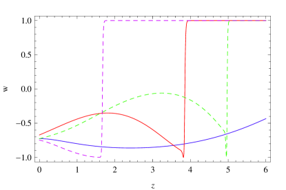
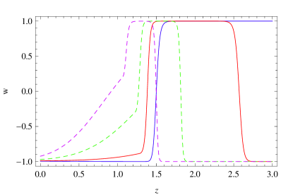
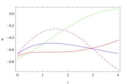
Figure 1: In Figs.1a, 1b and 1c we show the evolution of $w$ for a potential $V=V_{o}\phi^{-3/2}$, $V=V_{o}e^{-\phi/5}$ and $V=V_{o}\phi^{-4}e^{\phi^{2}/5}$, respectively, for different initial conditions.

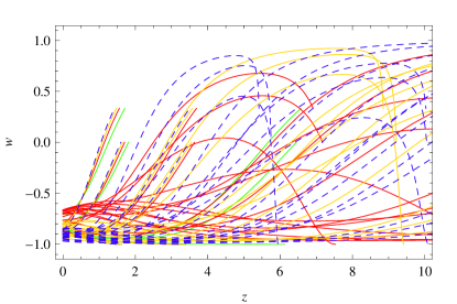
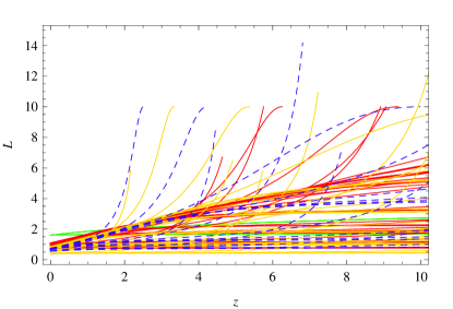
Figure 2: In fig.2a we show the evolution of $\hat{x},\hat{y}$ for different initial conditions. We also show in fig.2b,c $w$ and the corresponding $L$ as a function of z for different values of $\Gamma$ and $L_{i},\hat{x}_{i},\hat{y}_{i}$.

IV Scalar Field DE parametrization

The aim here is to test a wide class of DE models in order to constrain the dynamics of Dark Energy form the observational data. We could parameterize $w$ or $x$ with a single function in terms of the scale factor (c.f. Sec.IV.3) but as we have seen in eq.(21) we get a better understanding of the evolution of $\phi$ if we parameterize the functions $L$ and $y$.

In order to have the evolution of Dark Energy we need to either choose a potential $V(\phi)$ and solve eq.(III.1) or parameterize the EoS $w$ or $x$ as a function of the scale factor $a$. If we choose to parameterize $\zeta$ or $\lambda$ then we need to solve the differential equations eq.(III.1) or (III.2). On the other hand $L$ gives the evolution of $x$ and $w$ without needing to solve any differential equations and $L$ reduces to $\lambda$ (or $\zeta$) in the slow roll approximation. Therefore we propose here to use the exact equation for $w$ given in eq.(23) and parameterize the function $L$ and $y$.

A priori it is impossible to know how many free parameters has the potential $V(\phi)$ and since the evolution of different scalar field model requires the solve the eq.(III.1) and one has a difficult task to test a wide range of potentials $V$. The potential $V$ may involve a single term, as in a runaway potential as in $V=V_{o}\phi^{-n}$ or $V=V_{o}e^{-n\phi}$, or it may have different terms in the potential with the same order of magnitude as for example $V=A\phi^{-1}+Be^{n\phi}$ or $V=A\phi^{-1}+m^{2}\phi^{2}$ that may lead to a local minimum with $V\neq 0$.

In all these cases the evolution of $w$ would be different but still constrained to $-1\leq w\leq 1$, and in the slow roll approximation ($L\ll 1,x\ll 1$) one has $w\simeq-1+L/[3(1+y)]$ given by eq.(28). However, we do not know if there was a steep descent in $w$ or $x$ close to present time in such a way that for smaller $a<a_{o}$ the value of $w$ was much larger, e.g. $w$ close to 0, as matter, or even positive $w\simeq 1/3$, as radiation, with $L(a<a_{o})\gg L(a_{o})$ and the slow roll approximation may not be valid anymore. In this work, we would like to include a parametrization which includes also this kind of steep transition.

How many parameters should we use? We would say that we should use the minimum number of parameters as long as we still track the behavior of scalar fields and is generic enough to have different behavior for $w$ and allow the cosmological data to fix these parameters.

IV.1 Ansatz

We will propose an anzatz for $L$ and $y$ that covers the generic behavior of scalar field leading to an accelerating universe. If we want to have a constant EoS for DE at early times $z\gg 1$, as for example matter $w=0$ or radiation $w=1/3$, which are reasonable behavior for particles, we should choose $L$ proportional to $y$ for large $y$ with $L/y\rightarrow L_{1}$, or if we want $w\rightarrow-1$ at a large redshift the limit $L/y\rightarrow 0$ must be satisfied. We then propose to take

$$L=L_{o}+L_{1}\,y^{\xi}\,f(z)$$ (75)

with two free constant parameters $L_{o}$ and $L_{1}$, a transition function $f(z)$ constrained between $0\leq f(z)\leq 1$. The quantity $\xi$ takes the values $\xi=1$ and $\xi=0$ only and we do not consider it as a free parameter but more as two different ansatze for $L$, depending if we want $L$ to grow proportional to $y$ (i.e. $\xi=1$) or to a constant value in which case we take $\xi=0$. Since in the limit of large redshift $z\gg 1$ we have $y\gg 1$ and $L/y$ goes to a constant value $L_{1}$ or zero for $\xi=1,0$ respectively. This limit is independent of the functional form of $y$, since at large $y$ the EoS $w$ depends on $L/y\rightarrow L_{1}$ and the dependence on $y$ cancels out giving a constant value and a constant $w$ (c.f. eq.(31)). We therefore choose to take $y$ in eq.(75) as in eq.(54) with $w\simeq w_{o}$, i.e.

$$y=\frac{\rho_{m}}{V}=y_{o}\left(\frac{a}{a_{o}}\right)^{3w_{o}}=y_{o}(1+z)^{-3w_{o}}.$$ (76)

However, taking $y$ as in eq.(54) does not mean that $\rho_{\phi}\propto(a_{o}/a)^{3(1+w_{o})}$ since the kinetic energy $\dot{\phi}^{2}/2$, or equivalently $x$, may grow faster or slower than $V$. For $\xi=1$, eq.(75) allows a wide class of behaviors for $w$. If we want $w$ to increase to $w=0,1/3$ at earlier times we would take $L_{1}=6,12$, respectively, or since in many scalar field models the evolution of $w$ goes form $w_{o}$ to a region dominated by the kinetic energy density with $w=1$ and in this case we would should take $L_{1}\gg 1$. Of course a $w(z\gg 1)=1$ would only be valid for a limited period since $\Omega_{\phi}$ should not dominate the universe at early times. We have included in eq.(75) the case $\xi=0$ because we want to allow $w$ to increase from $w_{o}$ at small z and later go to $w\rightarrow-1$ (c.f. pink-dashed line in fig.(5)), since this is the behavior of potentials used as a models of DE as for example $V=V_{o}\phi^{-n},n=2/3$ derived from gauge group dynamics GDE.ax where the behavior of $w(z)$ close to present time depends on the initial conditions.

We propose to take the simple ansatz for the transition $f(z)$ given by

$$f(z)=\frac{(z/zt)^{k}}{1+(z/z_{t})^{k}},$$ (77)

with $f_{o}\equiv f(z=0)=0,f(z=z_{t})=1/2$ and $f_{i}\equiv f(z\gg 1)=1$. The transition function $f(z)$ given in eq.(77) has four free parameters $L_{o},L_{1},z_{t}$ and $k$. The parameters $L_{o}$ and $L_{1}$ give the EoS $w$ at present time and at large redshift $z\gg z_{t}$, while the transition epoch from $w_{o}$ to $w_{i}\equiv w(z\gg z_{t})$ is given by $z_{t}$ and $k$ sets the steepness of this transition. This parametrization has a simple expression in terms of z and it reduces to CPL CPL , i.e. $w=w_{o}+w_{a}(1-a)$), in the full slow roll approximation for $\xi=0$ and $z_{t}=1,k=1$ one has $f(z)=z/(1+z)=1-a$ and $L=L_{1}+L_{o}(1-a)$. Using eq.(39) we have $w\simeq-1+L/3=-1+(L_{o}+L_{1}f(z))/3$ and therefore we identify $w_{o}=-1+L_{o}/3$ and $w_{a}=L_{1}/3$. However, our parametrization given in eqs.(75) and (77) goes well beyond the CPL parametrization.

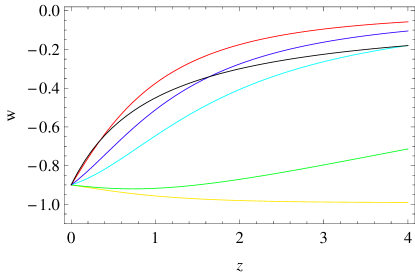
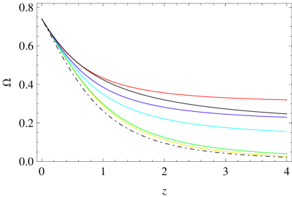
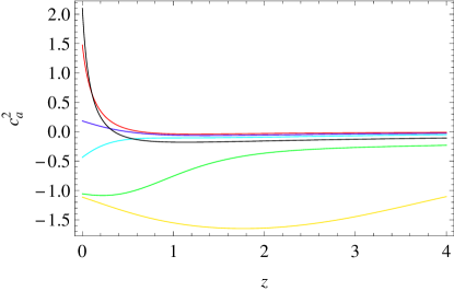
Figure 3: We show the evolution of $\Omega_{\phi}$, $w$ and $c_{a}^{2}$ for different models. We have taken $\xi=1$, $k=2$,$L_{1}=6$ with $z_{t}=0.1,1,$$2,10,100$ (red, dark blue, light blue, green and yellow, respectively). In black we have $w,\Omega_{w}$ using $w$ in eq.(83) and $\Omega_{cc}$ for a cosmological constant (black dot-dashed). We take in all cases $w_{o}=-0.9$, $\Omega_{\phi o}=0.74$ and $L_{1}=6$ giving $w_{i}=w(z\gg z_{t})=0$ for large z .

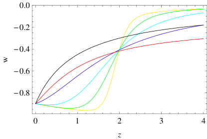
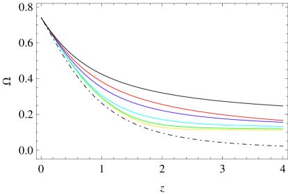
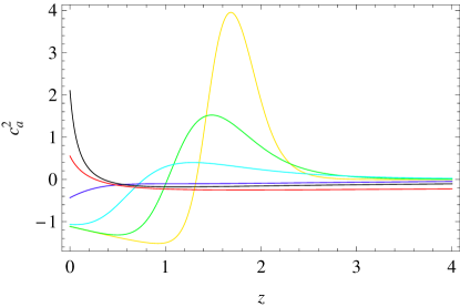
Figure 4: We show the evolution of $\Omega_{\phi}$, $w$ and $c_{a}^{2}$ for different models. We have taken $\xi=1$, $z_{t}=2$,$L_{1}=6$ fixed and $k=1/2,$ $2,$ $5,10,20$ (red, dark blue, light blue, green and yellow, respectively) In black we have $w,\Omega_{w}$ using $w$ in eq.(83) and $\Omega_{cc}$ for a cosmological constant (black dot-dashed). We take in all cases $w_{o}=-0.9$, $\Omega_{\phi o}=0.74$ and $L_{1}=6$ giving $w_{i}=w(z\gg z_{t})=0$ for large z .

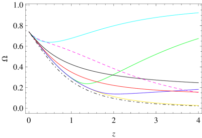
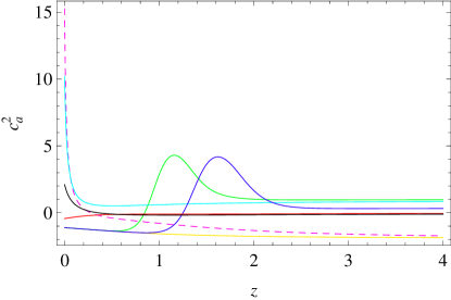
Figure 5: We show the evolution of $\Omega_{\phi}$, $w$ and $c_{a}^{2}$ for different models. We have taken $\xi=1$, $z_{t}=2$ fixed and $(k,L_{1})=(2,6),$$(20,12),(2,100),(20,1000),(20,0)$ (red, dark blue, light blue, green and yellow, respectively) and $\xi=0$ with $z_{t}=0.1,k=10,L1=12$ in pink-dashed line. In black we have $w,\Omega_{w}$ using $w$ in eq.(83) and $\Omega_{cc}$ for a cosmological constant (black dot-dashed). We take in all cases $w_{o}=-0.9$, $\Omega_{\phi o}=0.74$ and $L_{1}=6$ giving $w_{i}=w(z\gg z_{t})=0$ for large z .

IV.2 Initial Conditions and Free Parameters

Let us summarize the parameters and initial conditions of our parametrization. The EoS $w$ is only a function of $x$ and $x$ is a function of $L$ and $y$. From eq.(26) we see that $y$ depends on two parameters $w_{o}$ and $\Omega_{\phi o}$ (or equivalently on $y_{o},w_{o}$), since we are assuming a flat universe with DE and matter and $\Omega_{mo}=1-\Omega_{\phi o}$.

From eqs.(75) we have the conditions at present time as

$$y_{o}\equiv y(z=0)=\frac{\rho_{mo}}{V_{o}}=\frac{2}{(1-w_{o})}\frac{\Omega_{mo}}{\Omega_{\phi o}}$$ (78)

and from eq.(26) we express $L_{o}$ as a function of $w_{o}$ and $y_{o}$ we have and

$$L(z=0)=L_{o}=\frac{12(1+w_{o})+6y_{o}(1-w_{o}^{2})}{(1-w_{o})^{2}}$$ (79)

since $f(z=0)=0$. While the value at an early time we get

$$y_{i}\equiv y(z\gg 1)=\frac{2}{(1-w_{i})}\frac{\Omega_{mi}}{\Omega_{\phi i}}$$ (80)

and

$$L_{i}\equiv L(z\gg 1)=L_{o}+L_{1}y_{i}^{\xi}f_{i}=\frac{12(1+w_{i})+6y_{i}(1-w_{i}^{2})}{(1-w_{i})^{2}}\simeq\frac{6y_{i}(1+w_{i})}{(1-w_{i})},$$ (81)

with $f_{i}=f(z\gg 1)=1$. Since we expect to have negligible DE at early times we have $y_{i}\gg 1$ and we keep in the r.h.s. of eq.(81) only the term proportional to $y_{i}$. We see from this equation that for $\xi=1$ the value of $L_{1}$ is determined by the early time EoS $w_{i}$ with (c.f. eq.(31),

$$L_{1}=\frac{6(1+w_{i})}{1-w_{i}}$$ (82)

giving for example $L_{1}=6$ for $w_{i}=0$, $L_{1}=12$ for $w_{i}=1/3$ while $L_{1}=0$ requires $w_{i}\rightarrow-1$ and $L_{1}\gg 1$ has $w_{i}\rightarrow 1$. However, when $\xi=0$ we have the limit $L/y\rightarrow 0$ with $L_{i}=L_{o}+L_{1}$ a finite constant so eq.(81) requires $w_{i}=-1$ independently of the value of $L_{i}$.

From eq.(75) we have that $L$ depends on $y$ and $L_{o},L_{1},z_{t},k$ and $w_{o},\Omega_{\phi o}$. However, not all parameters are independent, since $L_{o}$ is a function of $w_{o},\Omega_{\phi o},L_{1},z_{t},q$ and we are left with $\Omega_{\phi o}$ and four parameters in $w$. To conclude, we can take the free parameters in the EoS as $w_{o}$, $w_{i}$, the transition redshift $z_{t}$ and the steepness of the transition $k$.

IV.3 Other Parameterizations

We present here some widely used parameterizations and we compare them with our DE parametrizations in this work. We begin with a simple DE parametrization CPL given in terms of only two parameters and widely used in most data analysis projects:

$$w(a)=w_{o}+w_{a}(1-a)=w_{o}+w_{a}\frac{z}{1+z}$$ (83)

with the derivative

$$\frac{dw}{da}=-w_{a},\;\;\;\;\frac{dw}{dz}=\frac{da}{dz}\frac{dw}{da}=(1+z)^{-2}w_{a}$$ (84)

Clearly $w$ in eq.(83) is convenient since it is a simple EoS and it has only two parameters. However, it may be too restrictive and we do not see a clear connection between the value of $w$ at small $a$ and its derivative at present time $w_{a}$. It has only 3 parameters $\Omega_{\phi o},w_{o},w_{a}$, two less than our model but our model has a much richer structure.

Another interesting parametrization was presented in corasaniti , with 4 free parameters. It is given by

$$w=w_{o}+(w_{i}-w_{o})\,G,\;\;G\equiv\frac{1+e^{a_{d}/d}}{1-e^{1/d}}\frac{1-e^{(1-a)/d_{i}}}{1+e^{(a_{d}-a)1/d}}$$ (85)

where $w_{o},w_{i},a_{d},d$ are constant parameters. The function $G$ is constraint between $0\leq G\leq 1$ with $G=0$ for $a\gg a_{d}$ and $G=1$ for $a\ll a_{d}$. Therefore $a_{d}$ is the scale factor where the transition of the EoS $w$ goes from $w_{o}$ to $w_{i}$ The parameter $d$ gives the width between the transition, for small $d$ the transition between $w_{o}$ and $w_{1}$ is steep. Even though w in eq.(85) gives a large variety of DE behavior corasaniti , since the sign of the slope is fixed our parametrization in eqs.(21) and (75) has a richer structure with the same number of parameters.

In the work of huang they have followed a similar motivation as in the present work. They have presented two DE parametrizations motivated by the dynamics of a scalar field. Their parametrizations have either two or three free parameters, and are given in eqs.(25) and (28) in the paper huang , respectively (they do not take $a_{eq}$ as a free parameter but we do think that it is an extra parameter). The two parameters involved determine the quantities $w_{i}(a\gg a_{o})$, which gives the EoS at an early time, and $\lambda(a_{eq})=V^{\prime}/V|_{a_{eq}}$ at DM-DE equality (i.e. $\Omega_{m}=\Omega_{de}$). In the second case, the parametrization also involves a term $\zeta_{s}$ (eq.(23) in huang ) which depends on a second derivative of $V$ and on the value of $\dot{\phi}/H$ at DM-DE equality. Since the functional form of the evolution of the EoS $w(a/a_{eq})$ is fixed in their parametrization the value of $w_{o}$ at present time is determined if we know the value of $a_{o}/a_{eq}$. Therefore, the quantity $a_{eq}$ must also be assumed as a free parameter. As in our present work, the system of equations do not close without the knowledge of the complete $V$ as a function of $\phi$. However, since we are both interested in extracting information from the observational data to determine the scalar potential the parametrization, given in eqs.(25) and (28) in huang , is an interesting proposal to study a wide range of potentials $V$. Here we have taken a different parametrization which has a closer connection to the scalar potential $V(\phi)$ given by eqs.(10) and (11).

IV.4 Results

We have plotted $w$ for different sets of the parameters in figs.(3),(4) and (5) to show how $w$ depends on $L_{o}$, $L_{1}$, $z_{t}$ and $k$. We notice that our parametrization in eq.(75) has a very rich structure allowing for $w$ to grow and or decrease at different redshifts. We have also plotted $\Omega_{\phi}$ and the adiabatic sound speed $c_{a}^{2}$ defined in eq.(V.2) for each model. We are showing some extreme cases which do not expect to be observational valid but we want to show the full extend of our parametrization. We have also included a cosmological constant ”C.C.” (black dot-dashed) in the figures of $\Omega_{\phi}$ and since $w_{cc}\equiv-1$ and $c_{a\,cc}^{2}=0$ we do not include them in the graphs for $w,c_{a}^{2}$. We also plotted $w,\Omega_{\phi},c_{a}^{2}$ (in black) for the parametrization in eq.(83) for comparison. We take in all cases $w_{o}=-0.9$, $\Omega_{\phi o}=0.74$.

In fig.(3) we show the evolution of $\Omega_{\phi}$, $w$ and $c_{a}^{2}$ for different models. We have taken $\xi=1,k=2,\,L_{1}=6$ with $z_{t}=0.1,1,2,10,100$ (red, dark blue, light blue, green and yellow, respectively). We take in all cases $L_{1}=6$ giving $w_{i}=w(z\gg z_{t})=0$. Notice that the yellow line the increase to $w=0$ does not show in the graph since $z_{t}=100$ and we plot $w$ only up to $z=4$. The slope in $w$ depends on the value of $z_{t}$ and since $k=2$ is not large the transition is not steep. The value of $\Omega_{\phi}$ decreases slower than for a C.C. and for smaller $z_{t}$ it decreases even more slowly, i.e when $w$ approaches zero faster.

In fig.(4) we show the evolution of $\Omega_{\phi}$, $w$ and $c_{a}^{2}$ for different models. In this case we have taken $\xi=1,z_{t}=2,\,L_{1}=6$ fixed with $w_{i}=0$ and we vary $k=1/2,2,5,10,20$ (red, dark blue, light blue, green and yellow, respectively). We clearly see in the evolution $w$ how the steepness of the transition depends $k$ and that $c_{a}^{2}$ has a bump at $z_{t}$ and it is more prominent for steeper transition. This is generic behavior and we could expect to see a signature of the transition in large scale structure as discussed in Sec.V.

In fig.(5) we show the evolution of $\Omega_{\phi}$, $w$ and $c_{a}^{2}$ and we take $\xi=1,z_{t}=2$ fixed and $(k,L_{1})=(2,6),(20,12),(2,100),(20,1000),(20,0)$ (red, dark blue, light blue, green and yellow, respectively) and $\xi=0$ with $z_{t}=0.1,q=10,L1=12$ (pink-dashed line). In this case we vary $L_{1}$ and we see that for large $L_{1}$ the EoS $w$ becomes bigger and it may approach $w\simeq 1$ (e.g. green line). Of course this case is not phenomenologically viable but we plot it to show the distinctive cases of our $w$ parametrization. Once again, a steep transition gives a bump in $c_{a}^{2}$. The pink-dashed line shows how $w$ can increase at low z and than approach $w=-1$.

We have seen that our parametrization gives a wide class of $w$ behavior, with increasing and decreasing $w$. From the observational data we should be able to fix the parameters of $L$ in eq.(75) and we could then have a much better understanding on the underlying potential $V(\phi)$.

V Perturbations

Besides the evolution of the homogenous part of Dark Energy $\phi(t)$, its perturbations $\delta\phi(t,x)$ are also an essential ingredient in determining the nature of DE. We work is the synchronous gauge and the linear perturbations with a line element $ds^{2}=a^{2}(-d\tau^{2}+(\delta_{ij}+h_{ij})dx^{i}dx^{j}$, where $h$ is the trace of the metric perturbations ma ; hu . In this sect.(V) a dot represents derivative with respect to conformal time $\tau$ and $\textsf{H}=\dot{a}/a=(da/d\tau)/a$ is the Hubble constant w.r.t. $\tau$, while $H=(da/dt)/a$

V.1 Scalar Field Perturbations

For a DE given in terms of a scalar field, the evolution requires the knowledge of $V$ and $V^{\prime}$ while the evolution of $\delta\phi(t,x)$ depends also on $V^{\prime\prime}$ through ma ; hu

$$\delta\ddot{\phi}+2\textsf{H}\delta\dot{\phi}+[k^{2}+a^{2}V^{\prime\prime}]\delta\phi=-\frac{1}{2}\dot{h}\dot{\phi}.$$ (86)

Eq.(86) can be expressed as a function of $a$ with $\dot{Y}=a\textsf{H}Y_{a}$ for $Y=\delta\phi,\phi,\textsf{H},h$ and the subscript $a$ means derivative w.r.t. $a$ (i.e. $Y_{a}\equiv dY/da$), giving

$$\delta\phi_{aa}+\left(\frac{3}{a}+\frac{\textsf{H}_{a}}{\textsf{H}}\right)\delta\phi_{a}+\left[\frac{k^{2}}{a^{2}\textsf{H}^{2}}+\frac{V^{\prime\prime}}{\textsf{H}^{2}}\right]\delta\phi=-\frac{1}{2}h_{a}\phi_{a}.$$ (87)

In the slow roll approximation we have

$$\left|\frac{V^{\prime\prime}}{3H^{2}}\right|=\Gamma x<3$$ (88)

where we have used eq.(21) and $\Gamma\equiv\frac{V^{\prime\prime}V}{V^{\prime 2}}$ given in eq.(73).

Eq.(88) implies that an EoS of DE between $-1\leq w\leq-1/3,0,1/3$, with $0\leq x\leq 1/2,1,2$, requires $\Gamma<3/x=6,3,3/2$, respectively. For a scalar field $\phi$ to be in the tracking regime one requires $\Gamma$ to be approximately constant with $\Gamma>1$ tracker . Therefore the regime $1<\Gamma<3/x$ allows a tracking behavior satisfying also the slow roll approximation. Here we are more interested in the late time evolution of DE and the tracking regime is not required and in fact we expect deviations from it. However, if $\Gamma$ is nearly constant the evolution of the perturbations in (87) are then given only in terms of $x$ and we can use our DE parametrization in eqs.(75) and (77) to calculate them.

We can express the slow roll parameter $\epsilon,\Upsilon$ in terms of $\Gamma$ and $L$ in the limit $q\ll 1$ as

$$\epsilon\equiv\frac{1}{2}\left(\frac{V^{\prime}}{V}\right)^{2}=\frac{\lambda^{2}}{2},\;\;\;\;\;\;\Upsilon\equiv\frac{V^{\prime\prime}}{V}=\Gamma\lambda^{2}$$ (89)

We have decided to use $L,\Upsilon$ instead of $\epsilon,\eta$ not to confuse the reader with the inflation parameters and the DE ones.

V.2 Fluid Perturbations

The evolution of the energy density perturbation $\delta=\delta\rho/\rho$, $\theta=k(1+w)v$, with $v$ is the velocity perturbation, are ma ; hu ; mukhanov ; bean

$$\dot{\delta}=-(1+w) \left(k^{2}+9\textsf{H}^{2}\,[c^{2}_{s}-c_{a}^{2}]\right)\frac{\theta}{k^{2}}-\frac{\dot{h}}{2}$$ (90)

$$-3\textsf{H}(c^{2}_{s}-w)\frac{\delta}{1+w}$$

$$\dot{\theta}=-\textsf{H}(1-3c^{2}_{s})\theta+c^{2}_{s}k^{2}\frac{\delta}{1+w},$$ (91)

and we do not consider an anisotropic stress. The evolution of the perturbations depends on three quantities hu ; bean

$$w = \frac{p}{\rho}$$ (92)

$$c^{2}_{a} = \frac{\dot{p}}{\dot{\rho}}=w+\dot{w}\frac{\rho}{\dot{\rho}}$$

$$= w-\frac{\dot{w}}{3\textsf{H}(1+w)}=w+\frac{x_{z}w_{x}}{3a(1+w)}$$

$$c^{2}_{s} = \frac{\delta p}{\delta\rho}$$ (94)

where $w$ is the EoS, H the Hubble constant in conformal time, $c^{2}_{a}$ is the adiabatic sound speed and $c^{2}_{s}$ is the sound speed in the rest frame of the fluid mukhanov ; hu . For a perfect fluid one has $c^{2}_{s}=c^{2}_{a}$ but scalar fields are not perfect fluids. The entropy perturbation $G_{i}$ for a fluid $\rho_{i}$ with $\delta_{i}=\delta\rho_{i}/\rho_{i}$ are

$$w_{i}G_{i}\equiv(c^{2}_{si}-c^{2}_{ai})\delta_{i}=\frac{\dot{p}_{i}}{\dot{\rho}_{i}}(\frac{\delta p_{i}}{\dot{p}_{i}}-\frac{\delta\rho_{i}}{\dot{\rho}_{i}})$$ (95)

where the quantities $G_{i}$ and $c^{2}_{ai}$ are scale independent and gauge invariant but $c^{2}_{si}$ can be neither ma ; bean . In its rest frame a scalar filed $\phi$ with a canonical kinetic term one has $c^{2}_{s}=\delta p/\delta\rho=1$ mukhanov ; hu . One can relate the rest frame $\hat{\delta},\hat{\theta}$ to an arbitrary frame $\delta,\theta$ by bean

$$\hat{\delta}=\delta+3\textsf{H}(1+w)\frac{\theta}{k^{2}}$$ (96)

and

$$\delta p=\hat{c}^{2}_{s}\delta\rho+(\hat{c}^{2}_{s}-c^{2}_{a})3\textsf{H}(1+w)\rho_{i}\frac{\theta}{k^{2}}.$$ (97)

As we see from eqs.(90)-(91) the evolution of $\delta$ depends on $c_{a}^{2},c^{2}_{s}$ and $w$. Using eq.(92) and since $w$ is a function of $x(a)$ we have

$$c^{2}_{a}=w+\frac{x_{z}w_{x}}{3a(1+w)}$$ (98)

with $w_{x}/(1+w)=2/[x(1+x)]$. From eqs.(23) and (21) we can express $c_{a}^{2}$ as a function of the parameters of $x$.

DE perturbations are important in distinguishing different DE models hu -DE.p and at the epoch where the universe is dominated by DM and DE the total perturbation is $\delta_{T}=\delta\rho_{T}/\rho_{T}=\Omega_{\rm DM}\delta\rho_{DM}+\Omega_{\rm DE}\delta\rho_{DE}$. If $\Omega_{\rm DE}$ is not much smaller than $\Omega_{\rm DM}$, i.e. at an epoch with low redshift z , then the perturbations of DE have an important contribution to $\delta_{T}$. Since for a scalar field $c^{2}_{a}\neq w$ and $c^{2}_{s}=1$ mukhanov ; hu we see from eqs.(90) and (91) that a bump in $c^{2}_{a}$ may give a significant contribution to the evolution of $\delta\rho_{DE}$ depending on the value of $\Omega_{\rm DE}$ (i.e. the redshift of the transition) and the steepness of the bump DE.p.sf ; DE.p .

Finally, we can relate $V^{\prime\prime}$ in terms of the adiabatic sound speed $c^{2}_{a}$ in eq.(V.2) and its time derivative, using $c^{2}_{a}=\dot{p}/\dot{\rho}=1+2V^{\prime}/3H(d\phi/dt)$, giving

$$\frac{dc^{2}_{a}}{dt}=\left(c^{2}_{a}-1\right)\left(\frac{V^{\prime\prime}}{V^{\prime}}-\frac{3H}{2}\left(\frac{2d\dot{H}}{3H^{2}}-(c^{2}_{a}+1)\right)\right)$$ (99)

and for $c^{2}_{a}\neq 1$ we can invert eq.(99) to give

$$\frac{V^{\prime\prime}}{V^{\prime}}=\frac{\Gamma\,V^{\prime}}{V}=\frac{1}{(c^{2}_{a}-1)}\frac{dc^{2}_{a}}{dt}-\frac{3H}{2}\left(w_{T}+c^{2}_{a}+2\right),$$ (100)

where we have used $\dot{H}=dH/dt=-(\rho_{T}+p_{T})/2=-3H^{2}(1+w_{T})/2$ with $\rho_{T},p_{T},w_{T}$ the total energy density, pressure and EoS, respectively. In our case we have $\rho_{T}=\rho_{m}+\rho_{\phi},\,p_{T}=p_{m}+p_{\phi}=p_{\phi}$ and using $\rho_{\phi}=V(1+x)$ and eqs.(11) and (16) we have

$$w_{T}\equiv\frac{p_{T}}{\rho_{T}}=w\Omega_{\phi}=\frac{w\rho_{\phi}}{3H^{2}}=\frac{w(1+x)}{1+x+y}=\frac{x-1}{1+x+y}.$$ (101)

With eq.(101) the l.h.s. of eq.(100) depends then only on $y,x$ and are fully determined by our parametrization. In the full slow roll approximation $\ddot{\phi}=0$ and one has $c_{a}^{2}=-1$.

VI Conclusions

We have presented a new parametrization of Dark Energy motivated by the dynamics of a canonical normalized scalar field minimally coupled to gravity. Our parametrization has allows for $w(z)$ to have a wide class of behavior in which it may grow and later decrease or other way around. The EoS $w(x(y,L))$ in eq.(23) is given in terms of the functions $L$ and $y$ and it is an exact equation, valid also when the slow roll approximation is not satisfied. The EoS $w$ is constrained between $-1\leq w\leq 1$ for any value of $x$, with $0\leq x$ by definition. The parametrization proposed is given in eqs.(75), (76) and (77), with $L=L_{o}+L_{1}\,y^{\xi}\,f(z)$ and a transition function $f(z)=\frac{(z/zt)^{k}}{1+(z/z_{t})^{k}}$, which has four free parameters: $L_{o},L_{1},z_{t},k$. The parameters $L_{o}$ and $L_{1}$ set the values of the EoS at present time $w_{o}$ and at an early time $w_{i}=w(z\gg z_{t})$, respectively (c.f. eq.(79) and (81). Therefore our EoS has four free parameters given by $w_{o}$ and $w_{i}$, the transition redshift $z_{t}$ at which the EoS goes from $w_{o}$ to $w_{i}$ plus the the steepness of the transition set by $k$. Besides studying the evolution of Dark Energy we also determined its perturbations from the adiabatic sound speed $c^{2}_{a}$ and $c^{2}_{s}$ given in eqs.(V.2) and (94), which are functions of $x$ and its derivatives. We have seen that a steep transition has a bump in $c^{2}_{a}$ and this should be detectable in large scale structure if it takes place at late times.

We can use the parametrization of $x(L,y)$ in eqs.(35), (75) and (76) and $c^{2}_{a}$ and $c^{2}_{s}$ in eqs.(V.2) and (94) without any reference to the underlying physics, namely the dynamics of the scalar field $\phi$, and the parametrization is well defined. However, it is when we interpret $x=\dot{\phi}^{2}/2V$ and $L=(V^{\prime}/V)^{2}A$ and $y=\rho_{m}/V$ that we are analyzing the evolution of a scalar field $\phi$ and we can connect the evolution of $w$ to the potential $V(\phi)$, once the free parameters are phenomenological determined by the cosmological data. The slow roll approximation is when we take $|q|\ll 1,A\simeq 1$.

To conclude, we have proposed a new parametrization of DE which has a rich structure, and the determination of its parameters will help us to understand the dynamics of Dark Energy.

Appendix A appendix

The parameter $|q\equiv\ddot{\phi}/V^{\prime}|$ is clearly smaller than one in the slow roll regime ($\ddot{\phi}<3H\dot{\phi}\simeq V^{\prime}$). Let us now determine the dependence of $q$ on the potential $V(\phi)$ and its derivatives. The evolution of $q$ is

$$\dot{q} = Hq_{N}=\frac{\dddot{\phi}}{V^{\prime}}-\frac{\ddot{\phi}\dot{\phi}}{V^{\prime 2}}$$ (102)

$$= 3H\left(-q+(1+q)\frac{\dot{H}}{3H^{2}}+2\Gamma x)\right)$$ (103)

where we used eq.(17),

$$\frac{\dddot{\phi}}{V^{\prime}} =-\frac{V^{\prime\prime}\dot{\phi}}{V^{\prime}}-\frac{3\dot{H}\dot{\phi}}{V^{\prime}}-\frac{3H\ddot{\phi}}{V^{\prime}}$$ (105)

$$=-3Hq+3H(1+q)\left(\frac{V^{\prime\prime}}{9H^{2}}+\frac{\dot{H}}{3H^{2}}\right),$$

and

$$\frac{V^{\prime\prime}}{9H^{2}}=\frac{\Gamma x}{3},\;\;\;\;\Gamma\equiv\frac{V^{\prime\prime}V}{V^{\prime 2}}.$$ (106)

We can estimate the value of $q$ if we drop the term proportional to $\dddot{\phi}$ in eq.(105) giving

$$q\simeq\frac{\frac{V^{\prime\prime}}{9H^{2}}+\frac{\dot{H}}{3H^{2}}}{1-(\frac{V^{\prime\prime}}{9H^{2}}+\frac{\dot{H}}{3H^{2}})}.$$ (107)

In a stable evolution of $\phi$ we have a positive $V^{\prime\prime}$ and since $\dot{H}$ is negative both terms have opposite signs, but of course we do not expect a complete cancelation of these terms. However both of them are smaller than one, since $0\leq-\dot{H}/3H^{2}<1/2$ for $x<1$ and $|V^{\prime\prime}/9H^{2}|=\Gamma x/3<1/3$ in the slow roll approximation. A tracker behavior requires $\Gamma>1$ tracker and $x<1/\Gamma<1$. Finally, the evolution of $L$ is given by $\dot{L}=H\,L_{N}=2\lambda\dot{\lambda}(1+q)^{2}+\lambda^{2}\dot{q}(1+q)=2L[\dot{\lambda}/\lambda+\dot{q}(1+q)]$,

$$\dot{L} = \frac{12HLx(1-\Gamma)}{(1+q)}+\frac{2L\dot{q}}{(1+q)}=3HL\left(\frac{2x-q}{1+q}+\frac{\dot{H}}{3H^{2}}\right)$$ (108)

$$= 3HL\left(\frac{2(q-x)(1+2x+2y)-y(1+q)}{2(1+q)(1+x+y)}\right).$$

We see that at $-1<q\leq x$ we have $\dot{L}<0$ giving a decreasing $L$ as a function of time or an increasing $L$ as a function of z . For $(q-x)/(1+q)>y/(1+2x+2y)$ or equivalently for $q>(y+2x(1+2x+2y))/(2+4x+3y)$ we have $\dot{L}>0$ and a decreasing $L$ as a function of z.

Instead of choosing a DE parametrization as in eq.(75) we could solve eqs.(102) and (108) for different potentials $V(\phi)$ or by taking different approximated solutions or ansatze for $\Gamma$. However, we choose to parameterize directly $L$ as in eq.(75). Still using $\dot{L}=\dot{a}L_{a}=aHL_{a}$ and $L_{1}y^{\xi}f=L-L_{o}$ we identify

$$(L-L_{o})\left(k\,f\left(\frac{a}{a_{t}}\right)^{k}-3\xi w_{o}\right)=3L\left(\frac{2x-q}{1+q}+\frac{\dot{H}}{3H^{2}}\right)$$ (109)

and the choices of $\Gamma$ and $q$ would fix the parameters $L_{o},k$ and $a_{t}$.

References

- (1)
- (2)
- (3) G. Hinshaw, D. Larson, E. Komatsu, D. N. Spergel, C. L. Bennett, J. Dunkley, M. R. Nolta and M. Halpern et al., arXiv:1212.5226 [astro-ph.CO].
- (4) P. A. R. Ade et al. [Planck Collaboration], arXiv:1502.01589 [astro-ph.CO], P. A. R. Ade et al. [Planck Collaboration], arXiv:1502.01590 [astro-ph.CO]. P. A. R. Ade et al. [ Planck Collaboration], arXiv:1303.5076 [astro-ph.CO].
- (5) L. Anderson, E. Aubourg, S. Bailey, F. Beutler, A. S. Bolton, J. Brinkmann, J. R. Brownstein and C. -H. Chuang et al., arXiv:1303.4666 [astro-ph.CO];
- (6) A. Conley, J. Guy, M. Sullivan, N. Regnault, P. Astier, C. Balland, S. Basa and R. G. Carlberg et al., Astrophys. J. Suppl. 192, 1 (2011) [arXiv:1104.1443 [astro-ph.CO]]; N. Suzuki, D. Rubin, C. Lidman, G. Aldering, R. Amanullah, K. Barbary, L. F. Barrientos and J. Botyanszki et al., Astrophys. J. 746, 85 (2012) [arXiv:1105.3470 [astro-ph.CO]].
- (7) J. Bock et al. (EPIC Collaboration), arXiv:0906.1188, BigBOSS Expermient Collaboration [arXiv. 1106.1706]; “Euclid Definition Study Report”arXiv:1110.3193 [astro-ph.CO]; B. M. Rossetto et al. [Dark Energy Survey Collaboration], arXiv:1104.4718 [astro-ph.GA].
- (8) E. J. Copeland, M. Sami, and S. Tsujikawa, Int. J. Mod. Phys. D 15, 1753 (2006).
- (9) M. Doran and G. Robbers, J. Cosmol. Astropart. Phys. 06 (2006) 026; E.V. Linder, Astropart. Phys. 26, 16 (2006); D. Rubin et al. , Astrophys. J. 695, 391 (2009) [arXiv:0807.1108]; J. Sollerman et al. , Astrophys. J. 703, 1374 (2009)[arXiv:0908.4276]; M.J. Mortonson, W. Hu, D. Huterer, Phys. Rev. D 81, 063007 (2010) [arXiv:0912.3816]; S. Hannestad, E. Mortsell JCAP 0409 (2004) 001 [astro-ph/0407259]; H.K.Jassal, J.S.Bagla, T.Padmanabhan, Mon.Not.Roy.Astron.Soc. 356, L11-L16 (2005); S. Lee, Phys.Rev.D71, 123528 (2005)
- (10) J. Z. Ma and X. Zhang, Phys. Lett. B 699 (2011) 233 [arXiv:1102.2671]; Dragan Huterer, Michael S. Turner Phys.Rev.D64:123527 (2001) [astro-ph/0012510]; Jochen Weller (1), Andreas Albrecht, Phys.Rev.D65:103512,2002 [astro-ph/0106079]
- (11) M. Chevallier and D. Polarski, Int. J. Mod. Phys. D10, 213 (2001); E. V. Linder, Phys. Rev. Lett. 90, 091301 (2003).
- (12) P. S. Corasaniti, B. A. Bassett, C. Ungarelli, and E. J. Copeland, Phys. Rev. Lett. 90, 091303 (2003);
- (13) Z. Huang, J. R. Bond, L.Kofman Astrophys.J.726:64,2011
- (14) B. Ratra and P. J. E. Peebles, Phys. Rev. D 37, 3406 (1988),C. Wetterich, Astron. Astrophys. 301, 321 (1995) [arXiv:hep-th/9408025].
- (15) P. Steinhardt, L.Wang, I.Zlatev, Phys.Rev.Lett. 82 (1999) 896; Phys.Rev.D 59(1999) 123504
- (16) A. de la Macorra and G. Piccinelli, Phys. Rev. D 61, 123503 (2000) [arXiv:hep-ph/9909459]; A. de la Macorra and C. Stephan-Otto, Phys. Rev. D 65, 083520 (2002) [arXiv:astro-ph/0110460].
- (17) A. de la Macorra, Phys. Rev. D 72, 043508 (2005) [arXiv:astro-ph/0409523]; A. De la Macorra, JHEP 0301, 033 (2003) [arXiv:hep-ph/0111292]; A. de la Macorra and C. Stephan-Otto, Phys. Rev. Lett. 87, 271301 (2001) [arXiv:astro-ph/0106316];
- (18) A. de la Macorra, Phys. Lett. B 585, 17 (2004) [arXiv:astro-ph/0212275],A. de la Macorra, Astropart. Phys. 33, 195 (2010) [arXiv:0908.0571 [astro-ph.CO]].
- (19) S. Das, P. S. Corasaniti and J. Khoury,Phys. Rev. D 73, 083509 (2006), arXiv:astro-ph/0510628; A. de la Macorra, Phys.Rev.D76, 027301 (2007), arXiv:astro-ph/0701635
- (20) A. de la Macorra, JCAP 0801, 030 (2008) [arXiv:astro-ph/0703702]; A. de la Macorra, Astropart. Phys. 28, 196 (2007) [arXiv:astro-ph/0702239].
- (21) C. Ma and E. Bertschinger, Astrophys. J. 455, 7 (1995)
- (22) J. Garriga and V. Mukhanov, Phys. Lett. B 458, 219 (1999)
- (23) W. Hu, D. Scott, N. Sugiyama and M. J. White, Phys. Rev. D 52, 5498 (1995), e-Print: astro-ph/9505043. W. Hu, Astrophys. J. 506 (1998) 485 [arXiv:astro-ph/9801234]. S. Bashinsky and U. Seljak, Phys. Rev. D 69, 083002 (2004)
- (24) R. Bean, O. Dore and , Phys. Rev. D 69, 083503 (2004) [astro-ph/0307100].
- (25) G. Ballesteros, A. Riotto and , Phys. Lett. B 668, 171 (2008) [arXiv:0807.3343 . L. R. Abramo, R. C. Batista, L. Liberato, R. Rosenfeld and , JCAP 0711, 012 (2007) [arXiv:0707.2882].
- (26) J. Liu, M. Li, X. Zhang and , JCAP 1106, 028 (2011) [arXiv:1011.6146 ]. U. Alam, Astrophys. J. 714, 1460 (2010) [arXiv:1003.1259]. R. de Putter, D. Huterer, E. V. Linder Phys. Rev. D 81, 103513 (2010) [arXiv:1002.1311]. H. K. Jassal, Phys. Rev. D 81, 083513 (2010) [arXiv:0910.1906].
- (27)