A new class of solutions of compact stars with charged distributions on pseudo-spheroidal spacetime
Abstract
In this paper a new class of exact solutions of Einstein’s field equations for compact stars with charged distributions is obtained on the basis of pseudo-spheroidal spacetime characterized by the metric potential , where and are geometric parameters of the spacetime. The expressions for radial pressure () and electric field intensity () are chosen in such a way that the model falls in the category of physically acceptable one. The bounds of geometric parameter and the physical parameters and are obtained by imposing the physical requirements and regularity conditions. The present model is in good agreement with the observational data of various compact stars like 4U 1820-30, PSR J1903+327, 4U 1608-52, Vela X-1, SMC X-4, Cen X-3 given by Gangopadhyay et al. [Gangopadhyay T., Ray S., Li X-D., Dey J. and Dey M., Mon. Not. R. Astron. Soc. 431 (2013) 3216]. When the model reduces to the uncharged anisotropic distribution given by Thomas and Pandya [Thomas V. O. and Pandya D. M., arXiv:1506.08698v1 [gr-qc](26 Jun 2015)].
1 Introduction
The equilibrium of a spherical distribution of matter in the form of perfect fluid is maintained by the repulsive pressure force against the gravitational attraction. For matter distribution in the form of dust, there is no such force to counter the gravitational attraction. In such situations, the collapse of the distribution to a singularity can be averted if the matter is accompanied by some electric charge. The Coulombian force of repulsion due to the presence of charge contributes additional force to the fluid pressure when the matter is in the form of perfect fluid.
A systematic study of electromagnetic fields in the context of general relativity was due to Rainich (1925). The equilibrium of charged dust spheres within the frame work of general relativity was examined critically by Papapetrou (1947) and Majumdar (1947). Bonner (1960, 1965) has shown that a spherical distribution of matter can keep its equilibrium if it is accompanied by certain modest electric charge. Stettner (1973) has shown that a uniform density fluid distribution accompanied by some surface charge is more stable than the one without charge. Krori and Barua (1975) obtained a singularity free solution for static charged fluid spheres. This solution has been analysed in detail by Juvenicus (1976). The solution obtained by Pant and Sah (1979) for static spherically symmetric relativistic charged fluid sphere has Tolman Solution VI as a particular case in the absence of charge.
Cooperstock and Cruz (1978) have studied relativistic spherical distributions of charged perfect fluids in equilibrium and obtained explicit solutions of Einstein - Maxwell equations in the interior of a sphere containing uniformly charged dust in equilibrium. Bonnor and Wickramsuriya (1975) have obtained a static interior dust metric with matter density increasing outward. Whitman and Burch (1981) have given a method for solving coupled Einstein - Maxwell equations for spherically symmetric static systems containing charge, obtained a number of analytic solutions and examined their stability. Conformally flat interior solutions were obtained by Chang (1983) for charged fluid as well as charged dust distributions.
Tikekar (1984) has studied some general aspects of spherically symmetric static distributions of charged fluids for specific choice of density and pressure. This solution admits Pant and Sah (1979) solution as a particular case. Patel and Mehta (1995) have obtained solutions of Einstein - Maxwell equations. Rao et al. (2000) have developed a formalism for generating new solutions of coupled Einstein - Maxwell equations.
The study of charged superdense star models compatible with observational data has generated deep interest among researchers in the recent past and a number of articles have been appeared in this direction Maurya and Gupta (2011a, b, c); Pant and Maurya (2012); Maurya et al. (2015). Theoretical investigations of Ruderman (1972) and Canuto (1974) suggest that matter may not be isotropic in high density regime and hence it is pertinent to study charged models incorporating anisotropy in pressure. Relativistic models of charged fluids distributions on spacetimes with spheroidal geometry have been studied by Patel and Kopper (1987), Tikekar and Singh (1998), Sharma et al. (2001), Gupta and Kumar (2005) and Komathiraj and Maharaj (2007).
Charged strange and quark star models have been studied by Sharma et al. (2006), and Sharma and Mukherjee (2001, 2002). The study of charged fluid distributions have been carried out recently by Maurya and Gupta (2011a, b, c), Pant and Maurya (2012) and Maurya et al. (2015).
In the present article, we have obtained a new class of solutions for charged fluid distribution on the background of pseudo spheroidal spacetime. Particular choices for radial pressure and electric field intensity are taken so that the physical requirements and regularity conditions are not violated. The bounds for the geometric parameter and the parameter associated with charge, are determined using various physical requirements that are expected to satisfy in its region of validity. It is found that these models can accommodate a number of pulsars like like 4U 1820-30, PSR J1903+327, 4U 1608-52, Vela X-1, SMC X-4, Cen X-3, given by Gangopadhyay et al. (2013). When the model reduces to the uncharged anisotropic distribution given by Thomas and Pandya (2015).
In section 2, we have solved Einstein - Maxwell equations and in section 3 the bounds for model parameters and are obtained using physical acceptability and regularity conditions. In section 4, we have displayed a variety of pulsars in agreement with the charged pseudo-spheroidal model developed. In section 5 we have examined various physical conditions throughout the distribution through the aid of numerical and graphical methods.
2 Spacetime Metric
A three-pseudo spheroid immersed in four-dimensional Euclidean space has the Cartesian equation
The sections are spheres of real or imaginary radius according as or while the sections , and are respectively, hyperboloids of two sheets.
On taking the parametrization
| (1) |
the Euclidean metric
takes the form
| (2) |
where and . The metric (2) is regular for all points with and call pseudo-spheroidal metric (Tikekar and Thomas (1998)).
We shall take the interior spacetime metric representing charged anisotropic matter distribution as
| (3) |
where and are geometric parameters and . This spacetime, known as pseudo-spheroidal spacetime, has been studied by number of researchers Tikekar and Thomas (1998, 1999, 2005); Thomas et al. (2005); Thomas and Ratanpal (2007); Paul et al. (2011); Paul and Chattopadhyay (2010); Chattopadhyay and Paul (2012) and have found that it can accommodate compact superdense stars.
Since the metric potential is chosen apriori, the other metric potential is to be determined by solving the Einstein-Maxwell field equations
| (4) |
where,
| (5) |
| (6) |
and
| (7) |
Here , , , and , respectively, denote the proper density, fluid pressure, unit-four velocity, magnitude of anisotropic tensor and a radial vector given by . denotes the anti-symmetric electromagnetic field strength tensor defined by
| (8) |
which satisfies the Maxwell equations
| (9) |
and
| (10) |
where denotes the determinant of , is four-potential and
| (11) |
is the four-current vector and denotes the charge density.
The only non-vanishing components of is . Here
| (12) |
and the total charge inside a radius is given by
| (13) |
The electric field intensity can be obtained from , which subsequently reduces to
| (14) |
The field equations given by (4) are now equivalent to the following set of the non-linear ODE’s
| (15) |
| (16) |
| (17) |
where we have taken
| (18) |
| (19) |
Because , the metric potential is a known function of . The set of equations (15) - (17) are to be solved for five unknowns , , , and . So we have two free variables for which suitable assumption can be made. We shall assume the following expressions for and with the central pressure
| (20) |
| (21) |
The expressions for and are so selected that it may comply with the physical requirement. A physically acceptable radial pressure should be finite at the centre decreasing radially outward and finally vanish at the boundary of the distribution. The gradient of is given by
| (22) |
It can be noticed from equation (20) that which is a finite quantity at It vanishes at which is taken as the boundary radius of the star. Further from equation (22) it can be noticed that is a radially decreasing function of . For a physically acceptable electric field intensity, and From equation (21), it is evident that is a monotonically increasing function of .
On substituting the values of and in (16) we obtain, after a lengthy calculation
| (23) | |||||
where is a constant of integration.
| (24) | |||||
The interior spacetime metric (24) is suitable to represent the charged fluid distribution if it match continuously with Riessner-Nordström metric
| (25) |
across the boundary . The continuity of metric coefficients across provide the estimates of the constant of integration and as
| (26) |
and
| (27) |
Here denotes the mass of the star inside the radius .
3 Physical Requirements and Bounds for Parameters
Now, equation (15) gives the density of the distribution as
| (28) |
The condition is clearly satisfied and gives the following inequality connecting and .
| (29) |
Since the inequality (29) implies
| (30) |
Differentiating (28) with respect to , we get
| (31) |
It is observed that and . In fact is a decreasing function of throughout the distributions.
The expression for is
| (32) | |||||
The condition at the boundary imposes a restriction on and respectively given by
| (33) |
and
| (34) |
The anisotropy can be written in the form as
| (35) |
The expression for is given by
| (36) | |||||
Evidently, the value of at the origin; and at the boundary gives the following bounds for with
| (37) |
| (38) |
a lower bound for .
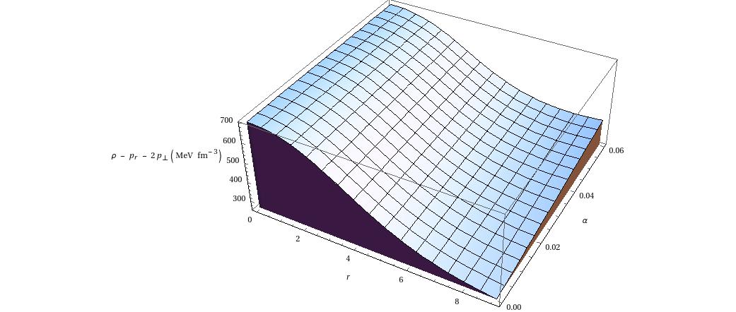
In order to examine the strong energy condition, we evaluate the expression at the centre and on the boundary of the star. It is found that, for a positivity of at the centre,
| (39) |
and gives the bound on and , namely
| (40) |
| (41) |
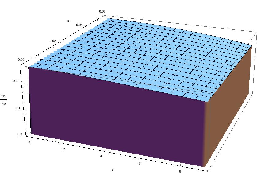
The expressions for adiabatic sound speed and in the radial and transverse directions, respectively, are given by
| (42) |
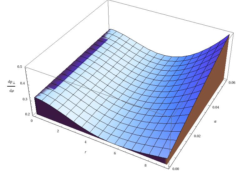
and
| (43) |
where and are given by expressions (31) and (36).
The condition gives the following bounds on with and ,
| (44) |
Moreover, leads to the following inequality
| (45) |
Further, , give the following bounds for , and
| (46) |
| (47) |
and
| (48) |
Moreover at the boundary , we have the following restrictions on and .
| (49) |
| (50) |
and
| (51) |
The necessary condition for the model to represent a stable relativistic star is that throughout the star. at gives a bound on with and ,
| (52) |
The upper limits of in the inequalities (29), (33), (37), (41), and (47) for different permissible values of are shown in Table 1. It can be noticed that the smallest bound for is given by (33).
The lower bounds of are calculated from (48) and (52). The upper bounds of are calculated from (34),(39),(44), (45), (48) & (51). They are listed in Table 2. The required lower bound for can be as taken as the largest values listed for each and the upper bound can be taken as the least values listed for each .
| Inequality Numbers | ||||||
|---|---|---|---|---|---|---|
| (29) | (33) | (37) | (41) | (47) | ||
| 1.8001 | 0.4898 | 0.0150 | 0.9999 | 7.9882 | 0.1600 | |
| 1.9001 | 0.5244 | 0.0179 | 0.9405 | 7.8029 | 0.2025 | |
| 2.0001 | 0.5556 | 0.0209 | 0.8888 | 7.6282 | 0.2501 | |
| 2.1001 | 0.5838 | 0.0239 | 0.8439 | 7.4632 | 0.3026 | |
| 2.2001 | 0.6094 | 0.0270 | 0.8047 | 7.3072 | 0.3601 | |
| 2.3001 | 0.6327 | 0.0301 | 0.7704 | 7.1594 | 0.4226 | |
| 2.4001 | 0.6540 | 0.0333 | 0.7405 | 7.0192 | 0.4901 | |
| 2.5001 | 0.6735 | 0.0364 | 0.7143 | 6.8861 | 0.5626 | |
| 2.6001 | 0.6914 | 0.0396 | 0.6913 | 6.7594 | 0.6401 | |
| 2.7001 | 0.7078 | 0.0427 | 0.6713 | 6.6388 | 0.7226 | |
| 2.8001 | 0.7230 | 0.0459 | 0.6537 | 6.5239 | 0.8101 | |
| 2.9001 | 0.7370 | 0.0490 | 0.6384 | 6.4142 | 0.9026 | |
| 3.0001 | 0.7500 | 0.0521 | 0.6250 | 6.3093 | 1.0001 | |
| 3.1001 | 0.7621 | 0.0552 | 0.6133 | 6.2091 | 1.1026 | |
| 3.2001 | 0.7733 | 0.0583 | 0.6032 | 6.1131 | 1.2101 | |
| 3.3001 | 0.7837 | 0.0613 | 0.5944 | 6.0211 | 1.3226 | |
| 3.3401 | 0.7876 | 0.0625 | 0.5912 | 5.9853 | 1.3690 | |
Similarly the lower bound for can be easily seen from the below Table 2.
| Inequality Numbers | |||||||||
|---|---|---|---|---|---|---|---|---|---|
| Lower Bounds | Upper Bounds | ||||||||
| (48) | (52) | (34) | (39) | (44) | (45) | (48) | (51) | ||
| 1.8001 | 0.0517 | 0.2852 | -0.4458 | 0.8001 | 2.0280 | 2.1409 | 1.2451 | 1.8315 | |
| 1.9001 | 0.0685 | 0.3176 | -0.4425 | 0.9001 | 2.2766 | 2.4551 | 1.4281 | 2.2249 | |
| 2.0001 | 0.0860 | 0.3500 | -0.4333 | 1.0001 | 2.5252 | 2.7837 | 1.6147 | 2.6409 | |
| 2.1001 | 0.1042 | 0.3826 | -0.4178 | 1.1001 | 2.7741 | 3.1262 | 1.8045 | 3.0756 | |
| 2.2001 | 0.1229 | 0.4152 | -0.3957 | 1.2001 | 3.0230 | 3.4824 | 1.9972 | 3.5253 | |
| 2.3001 | 0.1421 | 0.4479 | -0.3666 | 1.3001 | 3.2720 | 3.8520 | 2.1925 | 3.9860 | |
| 2.4001 | 0.1618 | 0.4806 | -0.3302 | 1.4001 | 3.5211 | 4.2349 | 2.3902 | 4.4537 | |
| 2.5001 | 0.1819 | 0.5134 | -0.2862 | 1.5001 | 3.7702 | 4.6308 | 2.5901 | 4.9247 | |
| 2.6001 | 0.2023 | 0.5462 | -0.2343 | 1.6001 | 4.0195 | 5.0395 | 2.7921 | 5.3952 | |
| 2.7001 | 0.2231 | 0.5790 | -0.1740 | 1.7001 | 4.2688 | 5.4610 | 2.9959 | 5.8619 | |
| 2.8001 | 0.2442 | 0.6119 | -0.1051 | 1.8001 | 4.5181 | 5.8951 | 3.2015 | 6.3216 | |
| 2.9001 | 0.2655 | 0.6449 | -0.0271 | 1.9001 | 4.7675 | 6.3416 | 3.4086 | 6.7715 | |
| 3.0001 | 0.2871 | 0.6778 | 0.0601 | 2.0001 | 5.0169 | 6.8005 | 3.6173 | 7.2091 | |
| 3.1001 | 0.3089 | 0.7108 | 0.1570 | 2.1001 | 5.2664 | 7.2716 | 3.8273 | 7.6325 | |
| 3.2001 | 0.3309 | 0.7438 | 0.2639 | 2.2001 | 5.5159 | 7.7549 | 4.0386 | 8.0398 | |
| 3.3001 | 0.3531 | 0.7768 | 0.3811 | 2.3001 | 5.7654 | 8.2502 | 4.2511 | 8.4296 | |
| 3.3401 | 0.3620 | 0.7900 | 0.4310 | 2.3401 | 5.8652 | 8.4517 | 4.3365 | 8.5804 | |
4 Application to Compact Stars
We shall use the charged anisotropic model on pseudo-spheroidal spacetime to strange star models whose mass and size are known. Consider the pulsar 4U 1820-30 whose estimated mass and radius are and . If we use these estimates in (27) with , we get which is well inside the permitted limits of . Similarly by taking the estimated masses and radii of some well-known pulsars like PSR J1903+327, 4U 1608-52, Vela X-1, SMC X-4 and Cen X-3, we have calculated the values of with for each of these stars. These estimates together with some relevant physical quantities like the central density surface density the compactification factor and the charge inside the star are displayed in Table 3. From this table it is evident that charged anisotropic models can accommodate the observational data of pulsars recently given by Gangopadhyay et al. (2013).
| STAR | ||||||||
|---|---|---|---|---|---|---|---|---|
| (MeV fm-3) | (MeV fm-3) | Coulombs | ||||||
| 4U 1820-30 | 2.718 | 1.58 | 9.1 | 1875.15 | 240.29 | 0.256 | 0.251 | 2.36 |
| PSR J1903+327 | 2.781 | 1.667 | 9.438 | 1806.35 | 226.58 | 0.261 | 0.242 | 2.45 |
| 4U 1608-52 | 3.010 | 1.74 | 9.31 | 2095.78 | 243.66 | 0.276 | 0.214 | 2.42 |
| Vela X-1 | 2.969 | 1.77 | 9.56 | 1947.00 | 229.38 | 0.273 | 0.218 | 2.48 |
| SMC X-4 | 2.230 | 1.29 | 8.831 | 1425.58 | 218.84 | 0.300 | 0.350 | 2.29 |
| Cen X-3 | 2.502 | 1.49 | 9.178 | 1610.99 | 223.03 | 0.239 | 0.287 | 2.38 |
5 Validation of Model for 4U 1820-30
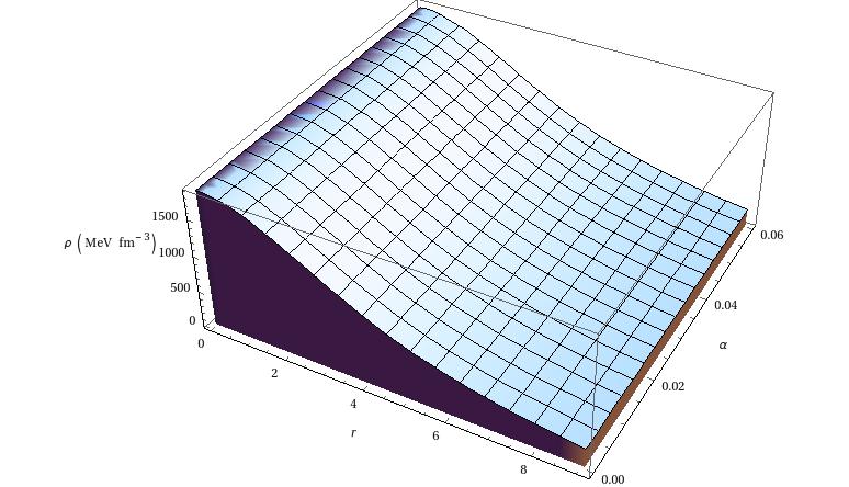
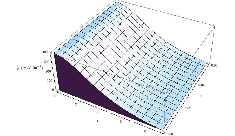
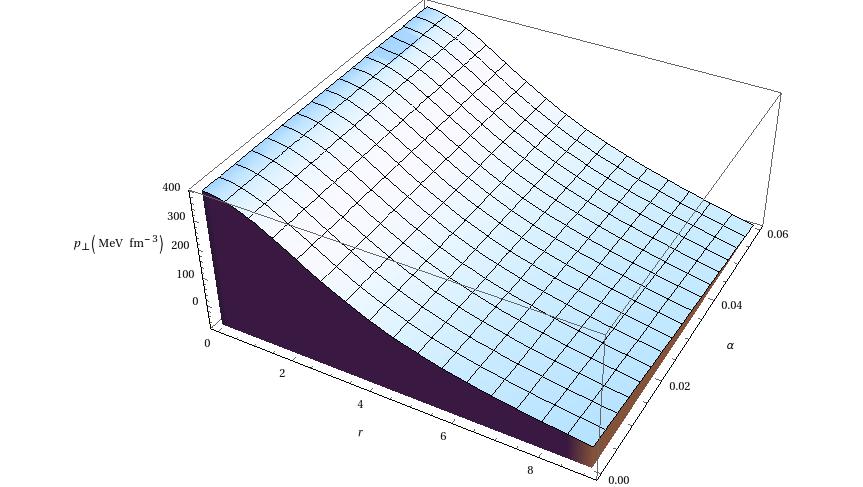
In order to examine the nature of physical quantities throughout the distribution, we have considered a particular pulsar 4U 1820-30, whose tabulated mass and radius are and respectively. From Table 3 it can be noticed that the corresponding values of with . We have shown the variations of density and pressures in both the charged and uncharged cases in Figure 1, Figure 2 and Figure 3. It can be noticed that the density is decreasing radially outward. Similarly the radial pressure and transverse pressure are decreasing radially outward.
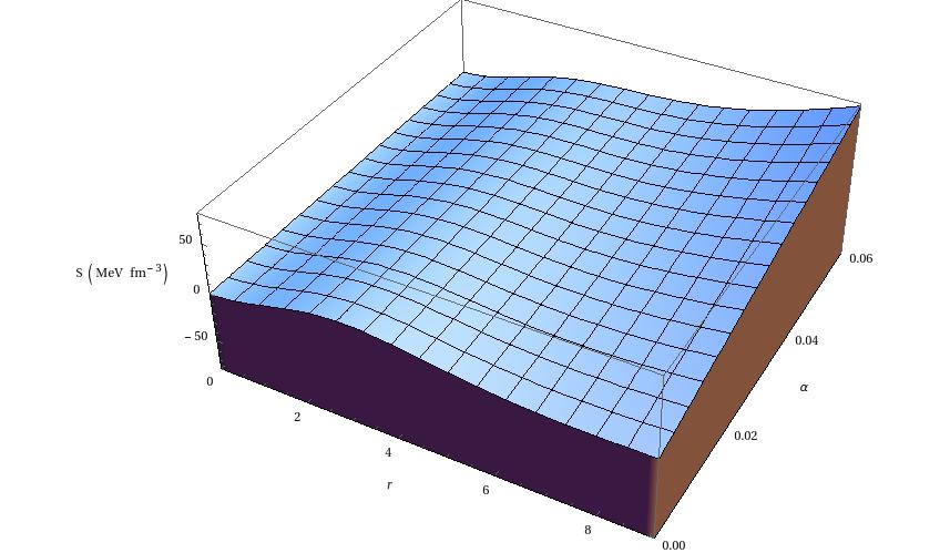
The variation of anisotropy shown in Figure 4 is initially decreasing with negative values reaches minimum and then increases. The square of sound speed in the radial and transverse direction (i.e. and ) are shown in Figure 5 and
Figure 6 respectively and found that they are less than 1, showing that the causality condition is fulfilled throughout. The graph of against radius is plotted in Figure 7. It can be observed that it is non-negative for and hence strong energy condition is satisfied throughout the star.
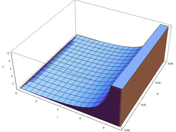
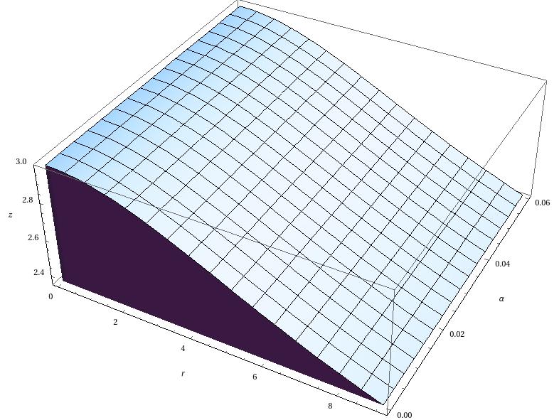
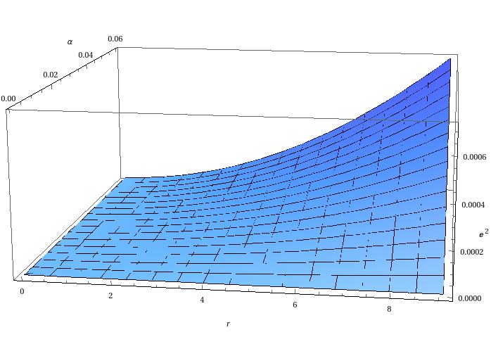
A necessary condition for the exact solution to represent stable relativistic star is that the relativistic adiabatic index given by should be greater than The variation of adiabatic index throughout the star is shown in Figure 8 and it is found that (Knutsen (1987)) throughout the distribution both in charged and uncharged case. For a physically acceptable relativistic star the gravitational redshift must be positive and finite at the centre and on the boundary. Further it should be a decreasing function of (Murad (2013)). Figure 9 shows that this is indeed the case. For a physically acceptable charged distribution, the electric field intensity should be an increasing function of (Murad (2013)). The variation of against is displayed in Figure 10. is found to be radially increasing throughout the distribution. The model reduces to the uncharged anisotropic distribution given by Thomas and Pandya (2015) when
Acknowledgement
The authors would like to thank IUCAA, Pune for the facilities and hospitality provided to them for carrying out this work.
References
- Paul and Chattopadhyay (2010) Chattopadhyay P. C. and Paul B. C., Pramana- J. of phys. 74 (2010) 513.
- Ruderman (1972) Ruderman R., Astro. Astrophys. 10 (1972) 427.
- Canuto (1974) Canuto V., Annu. Rev. Astron. Astrophys. 12 (1974) 167.
- Tikekar and Thomas (1998) Tikekar R. and Thomas V. O., Pramana- J. of phys. 50 (1998) 95.
- Tikekar and Thomas (2005) Tikekar R. and Thomas V. O., Pramana- J. of phys. 64 (2005) 5.
- Thomas et al. (2005) Thomas V. O., Ratanpal B. S. and Vinodkumar P. C., Int. J. Mod. Phys. D 14 (2005) 85.
- Thomas and Ratanpal (2007) Thomas V. O. and Ratanpal B. S., Int. J. Mod. Phys. D 16 (2007) 9.
- Komathiraj and Maharaj (2007) Komathiraj K. and Maharaj S. D., Intenational Journal of Modern Physics D 16 (2007) 1803.
- Paul et al. (2011) Paul B. C., Chattopadhyay P. K., Karmakar S. and Tikekar R., Mod. Phys. Lett. A 26 (2011) 575.
- Gangopadhyay et al. (2013) Gangopadhyay T., Ray S., Li X-D., Dey J. and Dey M., Mon. Not. R. Astron. Soc. 431 (2013) 3216.
- Tikekar and Thomas (1999) Tikekar R. and Thomas V. O., Pramana J. Phys. 52 (1999) 237.
- Chattopadhyay and Paul (2012) Chattopadhyay P. C., Deb R. and Paul B. C., Intenational Journal of Modern Physics D 21 (2012) 1250071.
- Bonner (1960) Bonner W. B., J. Phys. 160 (1960) 59.
- Bonner (1965) Bonner W. B., Mon. Not. R. Astron. Soc. 29 (1965) 443.
- Stettner (1973) Stettner R., Ann.Phys. 80 (1973) 212.
- Patel and Kopper (1987) Patel. L. K. and Kopper, Austr. J. Phys. 40 (1987) 441.
- Tikekar and Singh (1998) Tikekar R. and Singh G. P., Gravitation and Cosmology 4 (1998) 294.
- Sharma et al. (2001) Sharma R., Mukherjee S. and Maharaj S. D., Gen. Relativ. Gravit. 33 (2001) 999.
- Gupta and Kumar (2005) Gupta Y. K. and Kumar N., Gen. Relativ. Gravit. 37 (2005) 575.
- Sharma et al. (2006) Sharma R., Karmakar S. and Mukherjee S., Intenational Journal of Modern Physics D 15 (2006) 405.
- Sharma and Mukherjee (2001) Sharma R. and Mukherjee S., Modern Physics Letters A 16 (2001) 1049.
- Sharma and Mukherjee (2002) Sharma R. and Mukherjee S., Modern Physics Letters A 17 (2002) 2535.
- Maurya and Gupta (2011a) Maurya S. K. and Gupta Y. K., Astrophys. Space Sci. 331 (2011a) 135.
- Maurya and Gupta (2011b) Maurya S. K. and Gupta Y. K., Astrophys. Space Sci. 332 (2011b) 155.
- Maurya and Gupta (2011c) Maurya S. K. and Gupta Y. K., Astrophys. Space Sci. 333 (2011c) 415.
- Pant and Maurya (2012) Pant N. and Maurya S. K., App. Math. Comp. 218 (2012) 8260.
- Maurya et al. (2015) Maurya S. K. and Gupta Y. K. and Ray S., arXiv:1502.01915 [gr-qc] (2015).
- Rainich (1925) Rainich G. Y., Trans. Amer. Math. Soc. 27 (1925) 106.
- Papapetrou (1947) Papapetrou A., Proc. R. Irish Acad. A51 (1947) 191.
- Majumdar (1947) Majumdar S. D., Phys. Rev. 72 (1947) 390.
- Krori and Barua (1975) Krori K. D., and Barua J. J., Phys. A : Math. Gen. 8 (1975) 508.
- Juvenicus (1976) Juvenicus G. J. G., Phys. A : Math. Gen. 9 (1976) 2069.
- Pant and Sah (1979) Pant D. N. and Sah A. J., J. Math. Phys. 20 (1979) 2537.
- Cooperstock and Cruz (1978) Cooperstock F. I. and de la Cruz V., Gen. Rel. Grav. 9 (1978) 835.
- Bonnor and Wickramsuriya (1975) Bonnor W. B. and Wickramsuriya S.B.P., Mon. Not. Roy. Astron. Soc. 170 (1975) 643.
- Chang (1983) Chang B. S., Gen. Rel. Grav. 15 (1983) 293.
- Tikekar (1984) Tikekar R. S., J. Math. Phys. 25 (1984) 1481.
- Whitman and Burch (1981) Whitman P. G. and Burch R. C., Phys. Rev. D 24 (1981) 2049.
- Patel and Mehta (1995) Patel L. K. and Mehta N. P., J. Indian Math. Soc. 61 (1995) 95.
- Rao et al. (2000) Rao J. K., Annapurna M. and Trivedi M. M., Pramana J. Phys. 54 (2000) 215.
- Thomas and Pandya (2015) Thomas V. O. and Pandya D. M., arXiv:1506.08698v1 [gr-qc] (2015).
- Knutsen (1987) Knutsen H., Astrophys. Space Sci. 149 (1987) 38.
- Murad (2013) Murad M., Astrophys. Space Sci. 343 (2013) 187.