Numerical assessment of shearlet-based regularization in ROI tomography

Abstract

When it comes to computed tomography (CT), the possibility to reconstruct a small region-of-interest (ROI) using truncated projection data is particularly appealing due to its potential to lower radiation exposure and reduce the scanning time. However, ROI reconstruction from truncated projections is an ill-posed inverse problem, with the ill-posedness becoming more severe when the ROI size is getting smaller. To address this problem, both ad hoc analytic formulas and iterative numerical schemes have been proposed in the literature. In this paper, we introduce a novel approach for ROI CT reconstruction, formulated as a convex optimization problem with a regularized term based on shearlets. Our numerical implementation consists of an iterative scheme based on the scaled gradient projection (SGP) method and is tested in the context of fan beam CT. Our results show that this approach is essentially insensitive to the location of the ROI and remains very stable also when the ROI size is rather small.

1 Introduction

Computed Tomography (CT) is a noninvasive imaging technique designed to visualize the internal structure of a body or an object without surgical intervention or destructive material testing. To generate CT images, X-rays are propagated through the object and projections are collected from multiple views so that the density of the object can be reconstructed solving an appropriate inverse problem. The impact of CT has been enormous in areas including industrial nondestructive testing, security screening and medical diagnostics even though, in this last application, exposure to X-ray radiation comes with health hazards for patients. Luckily, in many biomedical situations, such as contrast-enhanced cardiac imaging or some surgical implant procedures, one is interested in examining only a small region-of-interest (ROI) with high resolution. Hence, there is no need to irradiate the entire body but only a smaller region, with the advantage of reducing radiation exposure and shortening the scanning time.

However, CT reconstruction is an ill-posed problem and the ill-posedness is even more severe when one attempts to solve the reconstruction problem from truncated projections [21], as in the case of ROI CT. Indeed, the direct application of classical reconstruction algorithms such as the Filtered Back-Projection (FBP) or the FDK algorithms [22] (with the missing projection data set to zero) typically produces unacceptable visual artifacts, and is more and more unstable to noise as the size of the ROI decreases.

During the last decade, a number of analytic and algebraic methods has been proposed to address the problem of ROI reconstruction from truncated projections [5]. In particular, it was shown that it is possible to derive analytic ROI reconstruction formulas from truncated data, even though such formulas usually require restrictive assumptions on the location of the ROI and depend on the acquisition setting [24, 25, 32]. For example, the Differentiated Back-Projection (DBP) methods [23, 6, 30] can be applied only if there exists at least one projection view in which the complete (i.e., non-truncated) projection data are available. Algebraic or iterative methods, on the other hand, are generally more flexible, since they can be applied to essentially any type of acquisition mode, also including several physical processes in the modeling. However, they are usually computationally more demanding, even if advances in high-performance computing make algebraic methods more and more competitive [2, 28]. Some common iterative algorithms, that have been adapted to ROI tomography, are the simultaneous iterative reconstruction technique (SIRT) [18], the maximum likelihood expectation-maximization algorithm (MLEM) [26] and the least-squares Conjugate Gradient (LSCG) method [19]. They typically involve some form of prior knowledge on the object attenuation function, or a regularization term to ensure a stable ROI reconstruction [17, 29, 31]. Anyway, the performance of existing methods is usually rather sensitive to the ROI size and the presence of noise.

In this paper, we address the ROI CT reconstruction problem using an iterative minimization algorithm formulated as a convex optimization problem with a regularized functional based on shearlets, a multiscale methods especially designed to sparsely approximate images with edges [9]. The approach here we consider relies on part on the setup recently proposed in [12], where the reconstruction method combines a data fidelity constraint to ensure that reconstructed projections matched the observed data inside the ROI and a data consistency condition to enforce that solutions are consistent with the tomographic reconstruction problem. Starting from this setup, we propose two formulations of the regularized reconstruction problem that we call implicit and explicit formulations. One main novelty of this paper is that our numerical implementation is based on the scaled gradient projection method [3], which is an accelerated first-order descent method for convex and non-convex objective functions. This method is particularly effective when the feasible region is given by “simple” constraints, that is, when projecting onto such a feasible region is not a heavy task. The numerical tests reported in this paper show that our algorithm produces accurate ROI reconstructions for any ROI location and also for ROI sizes that are small with respect to the field of view. We remark that a preliminary version of these results were recently presented in a conference paper [4].

The paper is organized as follows: in Section 2 we introduce the problem formulation in both the continuous and the discrete settings, translating it into two possible formulations of the objective function. Also, we quickly reiterate the mathematical background for both the shearlets and the SGP algorithm. In Section 3 we describe the setup for the simulated data and we recall the basics on distance-driven method [8]. Numerical experiments and results are given in Section 4. Finally, we draw some conclusions in Section 5.

2 SGP-shearlet approach for the region-of-interest tomography problem

In this section, we introduce the ROI CT problem in two dimensions. Our framework applies to different projection geometries, including parallel and fan-beam, and extends to higher dimensions. However, for brevity, we only consider here the two-dimensional case. We derive also a regularized reconstruction algorithm using two different formulations for the objective function. Our implementation is an iterative approach based on a first order descent method that can be applied to reach the unique solution of the problem.

2.1 Continuous setup: Radon transform and ROI solution uniqueness

The CT reconstruction problem consists in reconstructing a density function from a set of projections, obtained by measuring attenuation over straight lines. Mathematically, it becomes a “line-integral model” through the Radon transform notion. Given a function $f\in L^{1}(\mathbb{R}^{2})$, the Radon transform of $f$ at $(\theta,\tau)$ is the line integral of $f$ over the lines (or rays) $\ell(\theta,\tau)$ perpendicular to $\mathbf{e}_{\theta}=\bigl{(}\cos(\theta),\sin(\theta)\bigr{)}^{T}\in\mathbb{S}^{1}$ with (signed) distance $\tau\in\mathbb{R}$ from the origin:

$$\mathcal{R}f(\theta,\tau)=\int_{\ell(\theta,\tau)}f(\mathbf{x})\,d\mathbf{x}=\int_{\mathbb{R}^{2}}\delta(\tau-\mathbf{x}\cdot\mathbf{\mathrm{e}}_{\theta})\,f(\mathbf{x})\,d\mathbf{x},$$

where $\ell(\theta,\tau)=\{\mathbf{x}\in\mathbb{R}^{2}:\mathbf{x}\cdot\mathbf{e}_{\theta}=\tau\}$. Therefore, the Radon transform maps $f$ into the set of its linear projections defined on the tangent space $\mathcal{T}=\{(\theta,\tau):\theta\in[0,2\pi),\,\tau\in\mathbb{R}\}$. In what follows, we will refer to the Radon projections as the full sinogram and we shall denote it by:

$$y(\theta,\tau)=\mathcal{R}f(\theta,\tau),\quad\theta\in[0,2\pi),\,\tau\in\mathbb{R}.$$ (1)

We will refer to the domain of (1) as the projection domain and to the domain of the density function as the image domain.

In the ROI tomographic problem, projections are only collected for those rays meeting a region of interest inside the field of view. The goal is to recover the density function inside the ROI, while the rest of the function is essentially ignored. Denoting the ROI as $S\subset\mathbb{R}^{2}$, the set of ROI-truncated projections is identified to be the set

$$\mathcal{P}(S)=\{(\theta,\tau)\in\mathcal{T}:\ell(\theta,\tau)\cap S\neq\emptyset\}\subset\mathcal{T}.$$

Thus, the ROI reconstruction problem can be formulated as the problem of reconstructing the function $f$ restricted to the ROI $S$ from the truncated Radon projections:

$$y_{0}(\theta,\tau)=M(\theta,\tau)\,\mathcal{R}f(\theta,\tau),\qquad M(\theta,\tau)=1_{\mathcal{P}(S)}(\theta,\tau)$$ (2)

where $M$ is the mask function and $1_{A}$ is the indicator function of the set $A$. We will refer to $y_{0}$ as the truncated sinogram. In the following, we will assume that the ROI is a disk $S\subset\mathbb{R}^{2}$ with center $\mathbf{p}_{\text{ROI}}\in\mathbb{R}^{2}$ and radius $R_{\text{ROI}}\in\mathbb{R}$. Thus, $\mathcal{P}(S)=|\tau-\mathbf{p}_{\text{ROI}}\cdot\mathbf{e}_{\theta}|<R_{\text{ROI}}$. Clearly, more general convex ROIs can be handled by finding the minimal enclosing disk for this ROI and reconstructing the image for this disk.

A natural approach for obtaining a stable reconstruction of $f$ from equation (2) is by computing the least squares solution $\widehat{f}$

$$\widehat{f}=\arg\min_{f}\|M\mathcal{R}f-y_{0}\|_{2}^{2}.$$ (3)

However, the minimizer of this problem is not unique in general, since the set of solutions is the affine subspace

$$V=\{f\in L^{2}(\mathbb{R}^{2}):y=\mathcal{R}f\quad\text{and}\quad My=y_{0}\}.$$

Indeed, it is known that the solution of the ROI problem, in general, is not guaranteed to be unique [21]. Even when the uniqueness is ensured, the inversion of the Radon transform is an ill-posed problem and the ill-posedness may be more severe when projections are truncated, as in the case of the ROI CT problem. A classical approach to achieve uniqueness is by using Tikhonov regularization, which imposes an additional norm condition by searching for the minimum-norm solution. This norm condition can be applied in the image domain or in the projection domain, leading to different solutions, in general.

To define a norm condition in the projection domain, we can proceed as in [12] where the Riesz operator is used to relate the norm of $f$ to the norm of $\mathcal{R}f$. Namely, recall the definition of the Riesz potential operator $I^{-\alpha}$ for a function $g\in L^{2}(\mathcal{T})$:

$$\mathcal{F}(I^{\alpha}g)(\theta,\xi)=|\xi|^{-\alpha}\mathcal{F}g(\theta,\xi),\qquad\alpha<2.$$ (4)

Recall also the following formula [22]:

$$f=\frac{1}{4\pi}\mathcal{R}^{*}I^{-1}\mathcal{R}f,$$ (5)

where $\mathcal{R}^{*}$ is the adjoint operator of $\mathcal{R}$, also known as backprojection operator. Hence, we have:

$$\begin{split}\|f\|_{2}^{2}\;=\;\frac{1}{4\pi}\langle f,\mathcal{R}^{*}I^{-1}\mathcal{R}f\rangle\;&=\;\frac{1}{4\pi}\langle\mathcal{R}f,I^{-1}\mathcal{R}f\rangle\\ &=\;\frac{1}{4\pi}\langle I^{-\frac{1}{2}}\mathcal{R}f,I^{-\frac{1}{2}}\mathcal{R}f\rangle\;=\;\frac{1}{4\pi}\left\|I^{-\frac{1}{2}}\mathcal{R}f\right\|_{2}^{2}.\end{split}$$ (6)

Thus, we are lead to the following optimization problem:

$$\widehat{f}=\arg\min_{f}\;\bigl{\|}I^{-1/2}\mathcal{R}f\bigr{\|}_{2}^{2}\qquad\quad\text{s. t.}\quad y=\mathcal{R}f\quad\text{and}\quad My=y_{0}.$$ (7)

To formulate an objective function for the solution of the ROI reconstruction problem, we adopt the following observations from [12]. It is easy to see that

$$y=y_{0}+(1-M)\,y,$$ (8)

indicating that the ROI reconstruction problem can be viewed as an extrapolation problem where $y_{0}$, given on $\mathcal{P}(S)$, is to be extrapolated outside $\mathcal{P}(S)$. Clearly we cannot choose any extrapolated function $y$ outside $\mathcal{P}(S)$ but the following global constraint is needed

$$Rf=y.$$ (9)

Equation (9) ensures that $y$ belongs to range of the Radon transform of the density function $f\in L^{1}(\mathbb{R})\cap L^{2}(\mathbb{R})$. By applying $M$ and $1-M$ to the left-hand and right-hand sides of (9), respectively, we hence obtain the following equations (cf. [12]):

$$M\mathcal{R}f =M\,y=y_{0}\qquad\;\text{(data fidelity)}$$ (10)

$$(1-M)\mathcal{R}f =(1-M)\,y\qquad\text{(data consistency)}$$ (11)

The data fidelity equation defines a constraint inside the ROI and the data consistency equation enforces accurate reconstruction inside the ROI. These equations can be combined with regularization to obtain a computationally suitable algorithm for the ROI CT problem, as we shall see in section 2.2.

2.2 Discrete framework: explicit and implicit formulation of the objective function

To derive a discrete formulation for the ROI CT reconstruction framework, we need first to discretize equations (10) and (11). We shall denote by $K$ the number of projection angles and by $P$ the number of detector cells (i.e., samples along the detector array); $N$ is both the width and the height in pixels of the object to reconstruct. Given a projection geometry, the matrix $\mathbf{W}$ of the forward problem, that represents the map from the image domain to the projection domain, has dimensions $KP\times N^{2}$. The mask identifying the ROI is the diagonal matrix $\mathbf{M}$ of dimensions $KP\times KP$ whose entries are either 0 or 1. The unknown discrete density function $f$ to be reconstructed is represented as a vector $\mathbf{f}$ of length $N^{2}$ in which the entries are stacked column by column. Similarly, the full sinogram $y$ and the truncated sinogram $y_{0}$ are represented as vectors $\mathbf{y}$ and $\mathbf{y}_{0}$, respectively, of length $KP$, obtained by stacking the entries column by column. We recall that $\mathbf{y}$ and $\mathbf{y}_{0}$ are related to each other by the data fidelity equation

$$\mathbf{y}_{0}=\mathbf{My}=\mathbf{MWf},$$

and the data consistency equation, that sets the extrapolation scheme outside the ROI, reads as

$$(\mathbf{I}_{KP}-\mathbf{M})\mathbf{Wf}=(\mathbf{I}_{KP}-\mathbf{M})\mathbf{y},$$

where $\mathbf{I}_{KP}$ is the $KP\times KP$ identity matrix. As indicated above, data fidelity and data consistency equations need to be coupled with regularization to yield a unique solution. Thus, similarly to (7), we obtain the following discrete optimization problem:

$$\widehat{\mathbf{f}}=\arg\min_{\mathbf{f}}\|\mathbf{\Phi Wf}\|_{2}^{2}\qquad\quad\mbox{s. t.}\quad\mathbf{y}=\mathbf{Wf}\quad\mbox{and}\quad\mathbf{My}=\mathbf{y}_{0}$$ (12)

where $\mathbf{\Phi}$ is a discrete filter corresponding to the Riesz potential operator $I^{-\frac{1}{2}}$.

However, rather than requiring the exact equalities stated by data fidelity and data consistency equations, we shall minimize the $L^{2}$-norm error associated to them, according to a maximum likelihood approach. By exploiting this idea, we can state two different optimization problems and objective functions. On the one hand, we can consider the $L^{2}$-norm error of the data fidelity equation only and incorporate the data consistency information in the regularization term. In this case, the only variable we are minimizing on is the image $\mathbf{f}$ to be reconstructed. This approach yields:

$$\widehat{\mathbf{f}}=\arg\min_{\mathbf{f}\in\Omega_{\mathbf{f}}}\mathbf{\Psi}(\mathbf{f})$$

where

$$\mathbf{\Psi}(\mathbf{f})=\frac{1}{2}\|\mathbf{MWf}-\mathbf{y}_{0}\|_{2}^{2}+\lambda\,\|\mathbf{\Phi}((\mathbf{I}_{KP}-\mathbf{M})\mathbf{Wf}+\mathbf{y}_{0})\|_{2}^{2}.$$ (13)

We will refer to (13) as the implicit formulation, since the full sinogram $\mathbf{y}$ does not appear explicitly.

On the other hand, we can consider both the data fidelity and the data consistency $L^{2}$-norm errors into the objective function to assess if, by explicitly incorporating the extrapolation scheme in the minimization problem, we achieve a more accurate reconstruction. In this case, the image $\mathbf{f}$ to be reconstructed and the full sinogram $\mathbf{y}$ are both unknowns. This second approach yields:

$$\Bigl{(}\widehat{\mathbf{f}},\widehat{\mathbf{y}}\Bigr{)}=\arg\min_{\begin{subarray}{c}\mathbf{f}\in\Omega_{\mathbf{f}}\\ \mathbf{y}\geq\mathbf{0}\end{subarray}}\mathbf{\Psi}(\mathbf{f},\mathbf{y})$$

where

$$\begin{split}\mathbf{\Psi}(\mathbf{f},\mathbf{y})&=\frac{1}{2}\|\mathbf{MWf}-\mathbf{y}_{0}\|_{2}^{2}+\frac{1}{2}\|(\mathbf{I}_{KP}-\mathbf{M})(\mathbf{Wf}-\mathbf{y})\|_{2}^{2}\\ &\qquad+\lambda\,\|\mathbf{\Phi}((\mathbf{I}_{KP}-\mathbf{M})\mathbf{y}+\mathbf{y}_{0})\|_{2}^{2}.\end{split}$$ (14)

In contrast with the above formulation, we will refer to (14) as the explicit formulation. Notice that each term of the objective function is convex with respect to the unknowns. In both cases, $\lambda$ denotes the regularization parameter and the feasible region $\Omega_{\mathbf{f}}$ is either defined as $\mathbf{f}\geq 0$ or, when the maximum pixel value $L$ of the image happens to be known, as $0\leq\mathbf{f}\leq L$. Here the inequalities are meant component-wise. Notice also that each term of the objective function is convex with respect to the unknowns.

We will also include a smoothed total variation (TV) term [27] in the objective function to control oscillatory artifacts in the numerical solution. In conclusion, our objective functions are

$$\mathbf{\Psi}(\mathbf{f})=\dfrac{1}{2}\|\mathbf{MWf}-\mathbf{y}_{0}\|_{2}^{2}+\lambda\,\|\mathbf{\Phi}((\mathbf{I}_{KP}-\mathbf{M})\mathbf{Wf}+\mathbf{y}_{0})\|_{2}^{2}+\rho\;\text{TV}_{\delta}(\mathbf{f})$$ (15)

for the implicit formulation and

$$\begin{split}\mathbf{\Psi}(\mathbf{f},\mathbf{y})&=\frac{1}{2}\|\mathbf{MWf}-\mathbf{y}_{0}\|_{2}^{2}+\frac{1}{2}\|(\mathbf{I}_{KP}-\mathbf{M})(\mathbf{Wf}-\mathbf{y})\|_{2}^{2}\\ &\qquad+\lambda\,\|\mathbf{\Phi}((\mathbf{I}_{KP}-\mathbf{M})\mathbf{y}+\mathbf{y}_{0})\|_{2}^{2}+\rho\;\text{TV}_{\delta}(\mathbf{f})\end{split}$$ (16)

for the explicit one. Here, $\rho$ is a regularization parameter and $\delta$ is the TV smoothing parameter. TV was chosen since it is widely used in medical imaging. In the following, we will investigate if using the classical Tikhonov-like regularization term is superior to the TV minimization.

We remark that, in the absence of noise, the solution $\widehat{\mathbf{f}}$ is the same for both the implicit and the explicit cases (up to a vector in the nullspace of $\mathbf{W}$). However, in the presence of noise, the explicit formulation should benefit from the presence of the norm $\|\mathbf{W}\mathbf{f}-\mathbf{y}\|_{2}^{2}$ that is in general non-zero (and can be controlled using an appropriate stopping criterion, typically depending on the noise variance), forcing a more accurate reconstruction inside the ROI.

2.3 Regularization term: discrete shearlet transform

In the section above, the term $\mathbf{\Phi}$ was intentionally left unspecified. Indeed, in place of considering a straightforward matrix discretization of the Riesz potential operator, we will approximate it by using the discrete shearlet transform, a multiscale method which refines the conventional wavelet framework by combining multiscale analysis and directional sensitivity [14, 20]. For completeness, we briefly recall below the main ideas about shearlets.

Let $\phi\in L^{2}(\mathbb{R}^{2})$. A 2D affine family generated by $\phi$ is a collection of functions of the form:

$$\biggl{\{}\phi_{M,t}(x)=|\det(M)\,|^{-\frac{1}{2}}\phi\Bigl{(}M^{-1}(x-t)\Bigr{)}\;:\;M\in G,t\in\mathbb{R}^{2}\biggr{\}}$$

where $G$ is a subset of the group $GL_{2}(\mathbb{R})$ of invertible $2\times 2$ matrices. The function $\phi$ is called a 2D continuous wavelet if

$$g(x)=\int_{G}\int_{\mathbb{R}^{2}}\langle g,\,\phi_{M,t}\rangle\;\phi_{M,t}(x)\,dt\,d\lambda(M)\qquad\forall\;g\in L^{2}(\mathbb{R}^{2}),$$

where $\lambda(M)$ is an suitable measure on $G$. The corresponding 2D continuous wavelet transform of $g$ is the mapping

$$g\quad\mapsto\quad\mathcal{W}g(M,t)=\langle g,\,\phi_{M,t}\rangle,\qquad\quad M\in G,t\in\mathbb{R}^{2}.$$

Discrete wavelet transforms are obtained by discretizing $\mathcal{W}g(M,t)$ on an appropriate set. Usually, $M\in G$ and $t\in\mathbb{R}^{2}$ are replaced by $A^{j}$, $j\in\mathbb{Z}$, and $k\in\mathbb{Z}^{2}$, respectively, for appropriate choices of the matrix $A$. Shearlets are obtained from the 2D affine systems

$$\biggl{\{}\phi_{a,s,t}(x)={|\det(M_{a,s})\,|}^{-\frac{1}{2}}\phi\Bigl{(}M_{a,s}^{-1}(x-t)\Bigr{)}\;:\;M\in\Gamma,t\in\mathbb{R}^{2}\biggr{\}},$$

where $\phi\in L^{2}(\mathbb{R}^{2})$ and $\Gamma=\left\{M_{a,s}=\left(\begin{array}[]{cc}a&s\sqrt{a}\\ 0&\sqrt{a}\end{array}\right)\;:\;a\in\mathbb{R}^{+},s\in\mathbb{R}\right\}$ is a subset of $GL_{2}(\mathbb{R})$. Observe that the matrix $M_{a,s}$ is obtained by multiplying the anisotropic dilation matrix $A_{a}$ with the shear matrix $S_{s}$:

$$M_{a,s}=\left(\begin{array}[]{cc}a&s\sqrt{a}\\ 0&\sqrt{a}\end{array}\right)=\left(\begin{array}[]{cc}a&0\\ 0&\sqrt{a}\end{array}\right)\left(\begin{array}[]{cc}1&s\\ 0&1\end{array}\right)=:A_{a}S_{s}.$$

Here the variables $a\in\mathbb{R}^{+}$, $s\in\mathbb{R}$ and $t\in\mathbb{R}^{2}$ denote the scale, orientation and the spatial location, respectively. Thus, shearlets are formed by dilating, shearing and translating an appropriate mother shearlet function $\phi\in L^{2}(\mathbb{R}^{2})$ [15]. Roughly speaking, they are well localized waveforms whose orientation is controlled by the shear parameter $s$ and that become increasingly elongated at fine scales (as $a\rightarrow 0$). The continuous shearlet transform of $g$ is the map

$$g\quad\mapsto\quad\mathscr{S\!\!H}g(a,s,t)=\langle g,\,\phi_{a,s,t}\rangle,\qquad\quad a\in\mathbb{R}^{+},s\in\mathbb{R},t\in\mathbb{R}^{2}.$$

Discrete shearlet systems are formally defined by sampling a continuous shearlet systems on an appropriate discrete set. In particular, we choose

$$\begin{gathered}\biggl{\{}\phi_{j,k,m}(x)=2^{\frac{3}{4}j}\phi\Bigl{(}S_{k}A_{2^{j}}x-m\Bigr{)}\;:\;j,k\in\mathbb{Z},m\in\mathbb{Z}^{2}\biggr{\}}\\ \text{with $\phi$ s. t.}\quad\mathcal{F}(\phi)(\omega)=\mathcal{F}(\phi_{1})(\omega_{1})\;\mathcal{F}(\phi_{2})\left(\frac{\omega_{2}}{\omega_{1}}\right),\end{gathered}$$ (17)

where $\omega=(\omega_{1},\omega_{2})$, $\mathcal{F}(\phi_{1})$ is the Fourier transform of a wavelet function with compact support away from the origin and $\mathcal{F}(\phi_{2})$ is a compactly supported bump function with $\mathrm{supp}(\mathcal{F}(\phi_{2}))\subset[-1,1]$. Such a shearlet is called classical shearlet. Starting from a classical shearlet and under other suitable assumptions (see [16]), one can obtain a tight frame for $L^{2}(\mathbb{R}^{2})$. This indicates that the decomposition is invertible and the transformation is numerically well-conditioned. Notice that there exist several choices for $\phi_{1}$ and $\phi_{2}$ satisfying the classical shearlet definition. One possible choice is to set $\phi_{1}$ to be a Lemariè–Meyer wavelet and $\phi_{2}$ to be a spline bump function.

Summarizing, shearlets exhibit very appealing mathematical properties: they are well localized, namely they are compactly supported in the frequency domain and have fast decay in the spatial domain; the parabolic scaling allows to take care of the anisotropic structures; highly directional sensitivity is provided by the shearing parameter. Thanks to these properties, shearlets provide optimally sparse approximations with images containing $C^{2}$-edges, outperforming conventional wavelets [14]. This is potentially relevant in CT-like applications, since point-like structures in the image domain map onto sine-shaped curvilinear structures in the projection domain.

2.4 Scaled gradient projection method

In this section, we introduce our algorithm for the solution of the optimization problems (15)-(16), whose step-by-step description is given in Algorithm 1. The proposed method, called scaled gradient projection (SGP) method [3], is an iterative approach from the family of first-order descent methods that apply to convex (and non-convex), differentiable and constrained problems with “simple” feasible regions. This is indeed the case of our formulation, given that the feasible region $\Omega_{\mathbf{f}}$ is usually either a box or a non-negativity constraint and, as already indicated, our functionals are convex and differentiable.

Algorithm 1 Scaled Gradient Projection Method

Choose the starting point $\mathbf{f}^{(0)}\in\Omega_{\mathbf{f}}$, set the parameters $\beta,\gamma\in(0,1)$ and $0<\alpha_{\min}<\alpha_{\max}$. Fix a positive integer $\mu$.

for $k=0,1,2,\dots$ do

     Step 1. Choose the parameter $\alpha_{k}\in[\alpha_{\min},\alpha_{\max}]$ and the scaling matrix $D_{k}\in\mathcal{D}_{L}$ ;

     Step 2. Projection: $\mathbf{z}^{(k)}=\mathcal{P}_{\Omega_{f}}(\mathbf{f}^{(k)}-\alpha_{k}D_{k}\nabla\Psi(\mathbf{f}^{(k)}))$.  if $\mathbf{z}^{(k)}=\mathbf{f}^{(k)}$ then stop: $\mathbf{f}^{(k)}$ is a stationary point; end if

     Step 3. Descent direction: $\mathbf{d}^{(k)}=\mathbf{z}^{(k)}-\mathbf{f}^{(k)}$;

     Step 4. Set $\lambda_{k}=1$ and $\Psi_{\max}=\max_{0\leq j\leq\min(k,\mu-1)}\Psi(\mathbf{f}^{(k-j)})$;

     Step 5. Backtracking loop:

     if $\Psi(\mathbf{f}^{(k)}+\lambda_{k}\mathbf{d}^{(k)})\leq\Psi_{\max}+\beta\lambda_{k}\nabla\Psi(\mathbf{f}^{(k)})^{T}\mathbf{d}^{(k)}$ then

         go to Step 6;

     else

         set $\lambda_{k}=\gamma\lambda_{k}$ and go to Step 5;

     end if

     Step 6. Set $\mathbf{f}^{(k+1)}=\mathbf{f}^{(k)}+\lambda_{k}\mathbf{d}^{(k)}$.

end for

Some remarks about SGP are in order. When the objective function reads as in (15), the $(k+1)$-th iteration is

$$\mathbf{f}^{(k+1)}=(1-\lambda_{k})\,\mathbf{f}^{(k)}+\lambda_{k}\,\mathcal{P}_{\Omega_{\mathbf{f}}}\Bigl{(}\mathbf{f}^{(k)}-\alpha_{k}D_{k}\nabla\Psi(\mathbf{f}^{(k)})\Bigr{)}\qquad k=0,1,2,\ldots,$$ (18)

where $\lambda_{k}$, $\alpha_{k}$ are suitable steplengths, $D_{k}$ is the scaling matrix and $\mathcal{P}_{\Omega_{\mathbf{f}}}$ is the projector onto the feasible region. The main feature of this method consists in the combination of non-expensive diagonally scaled gradient directions with steplength selection rules specially designed for these directions. In details, any choice of the steplength $\alpha_{k}$ in a closed interval $[\alpha_{\min},\alpha_{\max}]\subset\mathbb{R}^{+}$ and of the scaling matrix $D_{k}$ in the compact set $\mathcal{D}_{L}$ is allowed, where $\mathcal{D}_{L}$ is the set of the symmetric positive definite matrices $D$ such that $\|D\|\leq L$ and $\|D^{-1}\|\leq L$, for a given threshold $L>1$. This is very important from a practical point of view because it makes their updating rules problem-related and performance-aware. In particular, SGP is equipped with an adaptive steplength selection based on the Barzilai-Borwein (BB) updating rules [1, 10]. In practice, by means of a variable threshold, one of the two different selection strategies

$$\alpha_{k}^{\text{BB1}} =\arg\min_{\alpha_{k}\in\mathbb{R}}\bigl{\|}B(\alpha_{k})\,\mathbf{s}^{(k-1)}-\mathbf{\zeta}^{(k-1)}\bigr{\|}$$

$$\alpha_{k}^{\text{BB2}} =\arg\min_{\alpha_{k}\in\mathbb{R}}\bigl{\|}\mathbf{s}^{(k-1)}-B(\alpha_{k})^{-1}\mathbf{\zeta}^{(k-1)}\bigr{\|}$$

is selected [11], where $B(\alpha_{k})=(\alpha_{k}D_{k})^{-1}$ approximates the Hessian matrix $\nabla^{2}\Psi(\mathbf{f}^{(k)})$, $\mathbf{s}^{(k-1)}=\mathbf{f}^{(k)}-\mathbf{f}^{(k-1)}$ and $\mathbf{\zeta}^{(k-1)}=\nabla\Psi(\mathbf{f}^{(k)})-\nabla\Psi(\mathbf{f}^{(k-1)})$. As far as the scaling matrix concerns, the updating rule for each entry $d_{i}^{(k)}$ is:

$$d_{i}^{(k)}=\min\left\{\sigma,\max\left\{\frac{1}{\sigma},\mathbf{f}_{i}^{(k)}\right\}\right\}\qquad i=1,\,\ldots,KP$$ (19)

where $\sigma$ is an appropriate threshold. We can setup the SGP method for the case of two unknowns, as in equation (16), by applying the SGP iteration to the “enlarge” variable $(\mathbf{f},\mathbf{y})$. This is accomplished by tacking a block-diagonal scaling matrix: the block corresponding to the image $\mathbf{f}$ reads as described above, while for the block corresponding to the full sinogram $\mathbf{y}$ we take $D_{k}=\mathbf{I}_{KP}$ for each $k=0,1,2,\ldots$. That is, the $(k+1)$-th iteration, with $k=0,1,2,\ldots$, is

$$\mathbf{f}^{(k+1)} =(1-\lambda_{k})\,\mathbf{f}^{(k)}+\lambda_{k}\,\mathcal{P}_{\Omega_{\mathbf{f}}}\Bigl{(}\mathbf{f}^{(k)}-\alpha_{k}D_{k}\nabla_{\mathbf{f}}\Psi(\mathbf{f}^{(k)},\mathbf{y}^{(k)})\Bigr{)}$$ (20)

$$\mathbf{y}^{(k+1)} =(1-\lambda_{k})\,\mathbf{y}^{(k)}+\lambda_{k}\,\mathcal{P}_{\mathbf{y}\geq 0}\Bigl{(}\mathbf{y}^{(k)}-\alpha_{k}\nabla_{\mathbf{y}}\Psi(\mathbf{f}^{(k)},\mathbf{y}^{(k)})\Bigr{)}$$ (21)

We notice also that global convergence properties are ensured by exploiting a nonmonotone line-search strategy along the feasible direction [13, 7]. Indeed, the nonmonotone line-search strategy, as implemented in step 5, ensures that $\Psi(\mathbf{f}^{(k+1)})$ ($\Psi(\mathbf{f}^{(k+1)},\mathbf{y}^{(k+1)})$, resp.) is lower than the maximum of the objective function on the last $\mu$ iterations; of course, if $\mu=1$ then the strategy reduces to the standard monotone Armijo rule. Moreover, since classical shearlets are tight frame, the equivalence $\mathbf{\Phi}^{T}\mathbf{\Phi}=\mathbf{I}_{KP}$ holds true and this allows to reduce the computational complexity of each algorithm iteration due to simpler updating rules.

Finally, notice that the SGP algorithm can be also used as an iterative regularization method applied to the un-regularized functional, by means of an early stopping technique.

3 Data simulation

To demonstrate and validate our approach, we use a synthetic data set known as modified Shepp-Logan phantom. It is available, for instance, in the Matlab Image Processing toolbox. All phantom data are simulated using the geometry of a micro-CT scanner used for real measurements. We simulate 2D fan-beam data over $182$ uniformly spaced angles over $2\pi$. The detector consists of $130$ elements with a pixel pitch of $0.8mm$. The distance between tube and detector is set to $291.20mm$ and the radius of rotation is $115.84mm$. The detector is offset by $1.5$ pixels. The 2D fan-beam geometry, represented by the matrix $\mathbf{W}$ introduced in section 2.2, is implemented by using the state-of-the-art method called distance-driven [8]. A brief introduction to its main mathematical ideas is reported in the section 3.1.

3.1 Distance-driven method

We recall that $\mathbf{W}$ is the $KP\times N^{2}$ matrix mapping the image domain into the projection domain. Every row of $\mathbf{W}$ contains weights that relate the pixel intensities in the image domain to the corresponding sample in the projection domain. Obviously, the value of each weight depends on the chosen interpolation scheme. The distance-driven method combines a highly sequential memory access pattern with relatively low arithmetic complexity, without introducing interpolation artifacts in the image or projection domains. Essentially, this approach is based on converting the projection problem into a 1D re-sampling problem. There are two main ingredients in the distance-driven method. The first one is the kernel operation:

$$\begin{gathered}b_{n}=\sum_{j}w_{j}c_{j}\qquad\text{with}\\ w_{j}=\dfrac{\bigl{[}\min(\xi_{m+1},\upsilon_{n+1})-\max(\xi_{m},\upsilon_{n})\bigr{]}_{+}}{\upsilon_{n+1}-\upsilon_{n}}\,,\quad[x]_{+}=\max(x,0)\,,\end{gathered}$$ (22)

which allows one to compute the destination signal values $\{b_{j}\}_{j}$ from the sample values $\{c_{i}\}_{i}$ of a source signal, the sample source locations $\{\xi_{i}\}_{i}$ and the sample destination locations $\{\upsilon_{j}\}_{j}$. The second element of the method is that there is a (possibly zero) length of overlap between each image pixel and each detector cell due to the bijection between the position on the detector and the position within an image row (or column). Thus, every point within an image row is uniquely mapped onto a point on the detector, and vice versa. In practice, to compute the overlap length, all pixel boundaries in an image row and all detector cell boundaries are mapped onto a common line, e.g., a line parallel to a coordinate axis. That is, each length of overlap is the interval length between two adjacent intersections, obtained by connecting the boundaries midpoints of all detector cells and pixels in a image row to the X-ray source and by computing the intercepts of these lines with the common axis. The final weights are achieved by normalizing the overlap length by the detector cell width. This corresponds exactly to apply the kernel operation from equation (22). In our case, $b_{n}$ is the theoretical (unblurred and noiseless) value measured at the $n$-th detector cell and $c_{j}$ is the estimate of the $j$-th pixel attenuation function. For example, if the $n$-th detector cell is “shadowed” by only two pixels in a row, equation (22) reads as:

$$b_{n}=\frac{\xi_{m+1}-\upsilon_{n}}{\upsilon_{n+1}-\upsilon_{n}}c_{m}+\frac{\upsilon_{n+1}-\xi_{m+1}}{\upsilon_{n+1}-\upsilon_{n}}c_{m+1}.$$

Notice that an efficient implementation of the distance-driven method can be achieved by using a vector-oriented approach instead of processing one pixel at a time. Indeed, one can update an entire row of the matrix (i.e., chosen one detector cell at a fixed angular view) in one shot by identifying all the pixels that shadow that detector cell and their corresponding length of overlap. Moreover, the detector can be chosen as the common line hence avoiding the need to calculate the projections of the detector cell boundaries. Finally, when the common line is not the detector, an effective choice is to adaptively select the common line by mapping onto the $x$-axis or $y$-axis, depending on the angular view.

4 Numerical experiments

$\gamma=0.5N$ $\gamma=0.3N$ $\gamma=0.15N$ value iter param value iter param value iter param PSNR SGP + Sh + TV 51.35 1277 $\lambda=5\cdot 10^{-4}$ 40.35 1951 $\lambda=5\cdot 10^{-4}$ 41.04 432 $\lambda=5\cdot 10^{-4}$ $\rho=0.01$ $\rho=1$ $\rho=1$ SGP + Sh 40.66 426 $\lambda=5\cdot 10^{-4}$ 35.85 745 $\lambda=5\cdot 10^{-4}$ 29.56 911 $\lambda=5\cdot 10^{-4}$ SGP + TV 47.58 841 $\rho=0.01$ 48.17 2526 $\rho=0.1$ 56.22 3998 $\rho=0.1$ SGP 48.88 7000 37.55 546 44.57 140 Rel. err. SGP + Sh + TV 0.01 1277 $\lambda=5\cdot 10^{-4}$ 0.10 1951 $\lambda=5\cdot 10^{-4}$ 0.24 432 $\lambda=5\cdot 10^{-4}$ $\rho=0.01$ $\rho=1$ $\rho=1$ SGP + Sh 0.04 426 $\lambda=5\cdot 10^{-4}$ 0.17 745 $\lambda=5\cdot 10^{-4}$ 0.91 911 $\lambda=5\cdot 10^{-4}$ SGP + TV 0.02 841 $\rho=0.01$ 0.04 2526 $\rho=0.1$ 0.04 3998 $\rho=0.1$ SGP 0.02 7000 0.14 546 0.16 140

Table 1: Optimal results for the implicit formulation of the objective function. The corresponding reconstructed images are reported in Figure 1.

In this section, we present extensive numerical results for the ROI CT reconstruction problem in the framework of 2D fan-beam geometry. All the algorithms were implemented in Matlab 8.1.0 and the experiments performed on a dual CPU server, equipped with two 6-cores Intel Xeon X5690 at 3.46GHz, 188 GB DDR3 central RAM memory and up to 12 TB of disk storage. The object to be imaged is the modified Shepp-Logan phantom sized $N\times N$ pixels with $N=128$. We assumed it to be placed in the first quadrant of the Cartesian coordinate system with the image lower left corner at the origin. Truncated projection data were obtained by discarding the samples outside the ROI projection $\mathcal{P}(S)$. We recall that this corresponds to a ROI disk in the image domain (see Section 2.1). In particular, we considered concentric ROI disks with decreasing radius $\gamma$, placed off-center with respect to the field of view. The results in this paper covers ROIs that are fully inside the object being imaged (in the hypothesis of the interior tomography problem). However, a larger radius that exceeds the object along one coordinate axis has been considered for comparison.

Numerical tests were performed to assess the best approach with respect to both the objective function and the regularization parameters. Tables 1 and 2 show some of the results for the implicit and the explicit formulations, respectively, compared against two state-of-the-art figures of merit, namely the peak-signal-to-noise ratio (PSNR) and the relative error. We recall that the PSNR, measured in dB, is defined as follows:

$$\text{PSNR}=10\log_{10}\Biggl{(}\dfrac{\text{MPV}^{2}}{\mathbf{e}_{\text{MSE}}}\Biggr{)}$$

where MPV is the maximum pixel value and $\mathbf{e}_{\text{MSE}}$ is the mean squared error. We stress that both PSNR and relative error are evaluated inside the ROI $S$ only. This is consistent with the motivation of ROI CT, that aims to recover the image inside the ROI only. The corresponding reconstructed images are reported in Figures 1 and 2.

We investigated the performance of the algorithm for the regularization parameter $\lambda=5\cdot 10^{\ell}$, $\ell={-4},{-3},\ldots,1$; for the TV parameter $\rho$ we sampled the values $10^{-2}$, $10^{-1}$ and $1$. We considered both the explicit and the implicit formulations of the objective function by designing different versions of the SGP method and by exploiting the early stopping technique. As far as the Tikhonov-like regularization term concerns, we also considered a one-level undecimated Daubechies 4 wavelet transform in place of classical shearlets. However, due to room constraint, only shearlet-based results are reported. In all experiments we found the latter to outperform the former on a visual basis, even if the figures of merit are comparable.

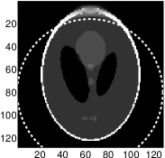
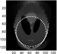
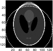
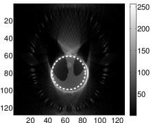
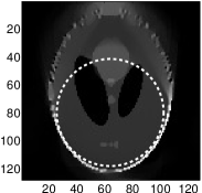
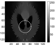
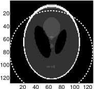
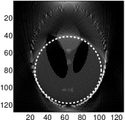
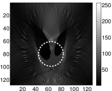
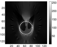
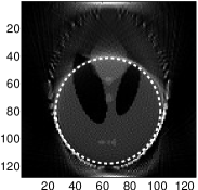
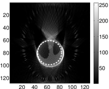
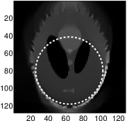
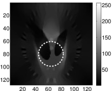
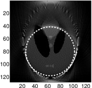
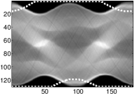
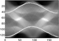
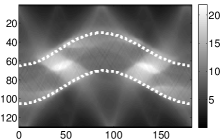
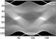
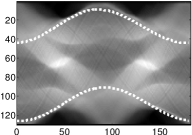
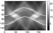
Figures 1 and 2 report the reconstructed images obtained for the implicit and the explicit formulations, respectively, and for decreasing radii. In details, in both figures, every row contains the reconstruction obtained with a different approach. Referring to Figure 1, in the first and in the second row, the objective function reads as in (15) and (13), respectively. In the third row, the objective function is obtained by dropping the Tikhonov-like regularization term of (15). In the fourth row, both the regularization and the TV terms are dropped and the reconstruction is obtained by exploiting the early stopping technique. The same holds true for Figure 2, where the referring equation for the first two rows are (16) and (14), respectively. Finally, in both figures, every column contains the reconstructions obtained for different radii: $\gamma=0.5N$ in the first column, $\gamma=0.3N$ in the second one and $\gamma=0.15N$ in the final one. In all of the pictures, the ROI is identified with a dashed white circle. Figure 3 collects the reconstructed sinograms obtained for the explicit formulation. We only report the reconstructions corresponding to the first and the third row of Figure 2, respectively. The circular ROI in the image domain corresponds to two sinusoidal dashed white lines in the projection domain. Finally, we report that further experiments with radius $\gamma$ equal to $0.25N$, $0.2N$ and $0.1N$ were performed: the corresponding figures of merit and reconstruction images do not appear here.

$\gamma=0.5N$ $\gamma=0.3N$ $\gamma=0.15N$ value iter param value iter param value iter param PSNR SGP + Sh + TV 45.69 1140 $\lambda=5\cdot 10^{-4}$ 40.35 3168 $\lambda=5\cdot 10^{-4}$ 34.63 604 $\lambda=5\cdot 10^{-4}$ $\rho=0.1$ $\rho=1$ $\rho=1$ SGP + Sh 41.50 1054 $\lambda=5\cdot 10^{-4}$ 34.86 1495 $\lambda=5\cdot 10^{-4}$ 28.46 2189 $\lambda=5\cdot 10^{-4}$ SGP + TV 49.59 1642 $\rho=0.01$ 41.51 2933 $\rho=1$ 39.55 556 $\rho=1$ SGP 45.01 7000 37.00 550 33.29 7000 Rel. err. SGP + Sh + TV 0.02 1140 $\lambda=5\cdot 10^{-4}$ 0.10 3168 $\lambda=5\cdot 10^{-4}$ 0.50 604 $\lambda=5\cdot 10^{-4}$ $\rho=0.1$ $\rho=1$ $\rho=1$ SGP + Sh 0.04 1054 $\lambda=5\cdot 10^{-4}$ 0.19 1495 $\lambda=5\cdot 10^{-4}$ 1.03 2189 $\lambda=5\cdot 10^{-4}$ SGP + TV 0.02 1642 $\rho=0.01$ 0.09 2933 $\rho=1$ 0.29 556 $\rho=1$ SGP 0.02 7000 0.15 550 0.59 7000

Table 2: Optimal results for the explicit formulation of the objective function. Corresponding reconstructed images are reported in Figure 2.

In Figure 1, we observe that, when the radius is as large as half the number of pixels of the image edge (panel (a), (d), (g) and (j)), all the reconstructions are good. The best approach for the objective function is to combine the Tikhonov-like regularization with the TV term (panel (a)), even if the error rate has the same magnitude for all possible approaches. Notice that, for all possible formulations, the values for the parameters $\lambda$ and $\rho$ are quite small: they are always the smallest ones of the investigated ranges. For smaller radii (panels (b), (e), (h) and (k) with $\gamma=0.3N$), we notice that the fundamental structures are detected by all the approaches, even if the TV-free approaches exhibits some checkerboard effects. The best reconstruction, with respect to both the figures of merit, is obtained by dropping only the Tikhonov-like regularization term (from the formulation (15)) and by setting to a medium value the TV regularization parameter $\rho$. Notice that the pure TV approach gains almost one order of magnitude for both figures of merit, with respect to the other approaches. The same considerations hold for the last case too. Indeed, when the radius decreases (panels (c), (f), (i) and (l) with $\gamma=0.15N$), the fundamental structures are still detected quite well in all the reported images, but also the checkerboard effect is still visible in the TV-free reconstructions. Even with this smaller radius, the optimal reconstruction is achieved for the same formulation of the objective function, and for the same value of the regularization parameter as the larger radius $\gamma=0.3N$. The relative error has the same magnitude as in the case $\gamma=0.3N$, gaining almost one order of magnitude with respect to the other approaches.

In Figure 2, we observe that the fundamental structures are consistently well detected in all reconstructions. The checkerboard effect persists in the TV-free reconstructions (second and fourth row), even if it is barely visible for the largest radius. The corresponding sinogram reconstructions reported in Figure 3 are accurate inside the ROI and therein they show no artifacts. This is clearly consistent with the good reconstruction of the corresponding images. The best approach for all radii, with respect to the figures of merit, is obtained by exploiting the purely TV-based approach. However, the largest radius (panel (g)) needs a small value for the regularization parameter ($\rho=0.01$) while the smaller ones (panels (h)-(i)) ask for a more severe TV regularization with $\rho=1$. While for $\gamma=0.5N$ the error rate (the PSNR, resp.) has the same magnitude for all possible approaches, for smaller radii the purely TV-based approach gains one order of magnitude. Notice that, even if figure (f) exhibits a definitely large relative error ($100\%$), on a visual basis the reconstruction is acceptable, or even good. Such a large relative error is probably due to the checkerboard effect (sub- or under-estimation of the pixel intensity).

In conclusion, observe that the pure TV approach, both in the implicit and in the explicit cases, is the one that requires more iterations to converge. As far as the early stopping approach concerns, when the number of iterations equals 7000, no semi-convergence property is observed, so the maximum number of iterations has been reached.

5 Conclusions

In this paper, we presented a numerical assessment of the solution of the ROI CT problem via a first-order iterative minimization method. We considered two different objective functions, each with a variable level of regularization aiming at ensuring stable reconstruction from truncated data. Numerical experiments have shown that our reconstruction algorithms are very satisfactory for all versions of the objective function; the main structures are recovered very accurately, with minimal ring artifacts. Using noiseless projection data, the purely TV-based approach performs slightly better than the shearlets-plus-TV approach, at least for smaller ROI radii (i.e., when the ROI is fully inside the field of view). We conjecture that this behavior might be dependent on the phantom features (which is piecewise constant) and may not hold for more general data. We expect that, using more realistic sinograms and including noise, the contribution of the shearlet term will become more relevant for the regularization. In fact, preliminary tests by the authors (not reported here) show that when projections are corrupted by noise the shearlet-based regularized reconstruction outperforms the one based solely on the TV term. Another important feature of our approach is that the performance of our ROI reconstructions algorithm is not sensitive to the location and size of the ROI and performs consistently well also for rather small ROI sizes, using both formulations of the objective function. In future work, we plan to consider more realistic phantoms, examine a different formulation of the optimization problem as indicated in section 2.1, and extend this method to the 3D case.

6 Acknowledgments

T.A.B., S.B. and G.Z. are supported by the Italian national research project FIRB2012, grant n. RBFR12M3AC, and by the local research project FAR2014 of the University of Ferrara. T.A.B. is supported by the Young Researchers Fellowship 2014 of the University of Ferrara. Also INdAM-GNCS is acknowledged. D.L. acknowledges partial support of NSF-DMS 1320910.

$\gamma=0.5N$ $\gamma=0.3N$ $\gamma=0.15N$ (a) (b) (c) (d) (e) (f) (g) (h) (i) (j) (k) (l)

Figure 1: Optimal reconstructions of the Shepp-Logan phantom for implicit formulation with decreasing radii: $\gamma=0.5N$ for (a), (d), (g) and (j), $\gamma=0.3N$ for (b), (e), (h) and (k), $\gamma=0.15N$ for (c), (f), (i) and (l). First row: shealerts and TV. Second row: just shearlets. Third row: just TV. Fourth row: early stopping only.

$\gamma=0.5N$ $\gamma=0.3N$ $\gamma=0.15N$ (a) (b) (c) (d) (e) (f) (g) (h) (i) (j) (k) (l)

Figure 2: Optimal reconstructions of the Shepp-Logan phantom for explicit formulation with decreasing radii: $\gamma=0.5N$ for (a), (d), (g) and (j), $\gamma=0.3N$ for (b), (e), (h) and (k), $\gamma=0.15N$ for (c), (f), (i) and (l). First row: shearlets and TV. Second row: just shearlets. Third row: just TV. Fourth row: early stopping only.

$\gamma=0.5N$ $\gamma=0.3N$ $\gamma=0.15N$ (a) (b) (c) (d) (e) (f)

Figure 3: Optimal reconstructions of the sinogram of the Shepp-Logan phantom for explicit formulation with decreasing radii: $\gamma=0.5N$ for (a) and (d), $\gamma=0.3N$ for (b) and (e), $\gamma=0.15N$ for (c) and (f). First row: shearlets and TV. Second row: just TV.

References

- Barzilai and Borwein [1988] J. Barzilai, J.M. Borwein, Two point step size gradient methods, IMA J. Numer. Anal. 8 (1988) 141–148.
- Beister et al. [2012] M. Beister, D. Kolditz, W. Kalender, Iterative reconstruction methods in x-ray ct, Phys. Med. 28 (2012) 94–108.
- Bonettini et al. [2009] S. Bonettini, R. Zanella, L. Zanni, A scaled gradient projection method for constrained image deblurring, Inverse Problems 25 (2009) 015002.
- Bubba et al. [2015] T. Bubba, D. Labate, G. Zanghirati, S. Bonettini, B. Goossens, Shearlet-based regularized ROI reconstruction in fan beam computed tomography, in: SPIE Optics & Photonics, Wavelets And Applications XVI, volume 9597, San Diego, CA, USA, p. 95970K.
- Clackdoyle and Defrise [2010] R. Clackdoyle, M. Defrise, Tomographic reconstruction in the 21st century. region-of-interest reconstruction from incomplete data, IEEE Signal Processing 60 (2010) 60–80.
- Clackdoyle et al. [2004] R. Clackdoyle, F. Noo, J. Guo, J. Roberts, Quantitative reconstruction from truncated projections in classical tomography, IEEE Trans. Nuclear Science 51 (2004) 2570–2578.
- Dai and Fletcher [2005] Y.H. Dai, R. Fletcher, On the asymptotic behaviour of some new gradient methods, Math. Programming 103 (2005) 541–559.
- De Man and Basu [2004] B. De Man, S. Basu, Distance-driven projection and backprojection in three dimensions, Physics in Medicine and Biology 7 (2004) 2463–2475.
- Easley et al. [2008] G.R. Easley, D. Labate, W. Lim, Sparse directional image representations using the discrete shearlet transform, Appl. Comput. Harmon. Anal. 25 (2008) 25–46.
- Fletcher [2001] R. Fletcher, On the Barzilai-Borwein method, Technical Report NA/207, Technical Report, Department of Mathematics, University of Dundee, Dundee, UK, 2001.
- Frassoldati et al. [2008] G. Frassoldati, G. Zanghirati, L. Zanni, New adaptive stepsize selections in gradient methods, J. Industrial and Management Optim. 4 (2008) 299–312.
- Goossens et al. [2014] B. Goossens, D. Labate, B. Bodmann, Region-of-interest computed tomography by regularity-inducing convex optimization, submitted (2014).
- Grippo et al. [1986] L. Grippo, F. Lampariello, S. Lucidi, A nonmonotone line-search technique for newton s method, SIAM J. Numer. Anal. 23 (1986) 707–716.
- Guo and Labate [2007] K. Guo, D. Labate, Optimally sparse multidimensional representation using shearlets, SIAM J. Math. Analysis 39 (2007) 298–318.
- Guo et al. [2009] K. Guo, D. Labate, W.Q. Lim, Edge analysis and identification using the continuous shearlet transform, Applied and Computational Harmonic Analysis 27 (2009) 24–46.
- Guo et al. [2006] K. Guo, D. Labate, W.Q. Lim, G. Weiss, E. Wilson, Wavelets with composite dilations and their MRA properties, Applied and Computational Harmonic Analysis 20 (2006) 202–236.
- Hamelin et al. [2010] B. Hamelin, Y. Goussard, J. Dussault, G. Cloutier, G. Beaudoin, G. Soulez, Design of iterative roi transmission tomography reconstruction procedures and image quality analysis, Medical Physics 37 (2010) 4577–4589.
- Herman and Lent [1976] G.T. Herman, A. Lent, Iterative reconstruction algorithms, Computers in Biology and Medicine 6 (1976) 273–294.
- Hestenes and Stiefel [1952] M. Hestenes, E. Stiefel, Methods of conjugate gradients for solving linear systems, Journal of Research of the National Bureau of Standards 6 (1952) 409–436.
- Kutyniok and Labate [2012] G. Kutyniok, D. Labate, Shearlets: Multiscale Analysis for Multivariate Data, Springer, 2012.
- Natterer [2001] F. Natterer, The Mathematics of Computerized Tomography, SIAM: Society for Industrial and Applied Mathematics, 2001.
- Natterer and Wubbeling [2001] F. Natterer, F. Wubbeling, Mathematical Methods in Image Reconstruction, SIAM: Society for Industrial and Applied Mathematics, 2001.
- Noo et al. [2004] F. Noo, R. Clackdoyle, J. Pack, A two-step hilbert transform method for 2d image reconstruction, Physics in Medicine and Biology 49 (2004) 3903–3923.
- Noo et al. [2002] F. Noo, M. Defrise, R. Clackdoyle, H. Kudo, Image reconstruction from fan-beam projections on less than a short scan, Physics in Medicine and Biology 47 (2002) 2525–2546.
- R.Clackdoyle and Noo [2004] R.Clackdoyle, F. Noo, A large class of inversion formulae for the 2-d radon transform of functions of compact support, Inverse Problems 20 (2004) 1281–1291.
- Shepp and Vardi [1982] L. Shepp, Y. Vardi, Maximum likelihood reconstruction for emission tomography, IEEE Trans Med Imaging 1 (1982) 113–122.
- Vogel [2002] C. Vogel, Computational methods for inverse problems, SIAM Philadelphia, 2002.
- Yan et al. [2010] G. Yan, J. Tian, S. Zhu, C. Qin, Y. Dai, F. Yang, D. Dong, P. Wu, Fast Katsevich algorithm based on GPU for helical cone-beam computed tomography, Information Technology in Biomedicine, IEEE Transactions on 14 (2010) 1053–1061.
- Yang et al. [2010] J. Yang, H. Yu, M. Jiang, G. Wang, High-order total variation minimization for interior tomography, Inverse Problems 26 (2010) 035013.
- Zhang and Zeng [2007] B. Zhang, G. Zeng, Two dimensional iterative region of iterest reconstruction from truncated projection data, Medical Physics 34 (2007) 935–944.
- Ziegler et al. [2008] A. Ziegler, T. Nielsen, M. Grass, Iterative reconstruction of a region of interest for transmission tomography, Medical Physics 35 (2008) 1317–1327.
- Zou et al. [2005] Y. Zou, X. Pan, E. Sidky, Image reconstruction in regions-of-interest from truncated projections in a reduced fan-beam scan, Phys. Med. Biol. 50 (2005) 13–28.