challenge.icon-fet.eu

Lars Kotthoff

1 Submissions

The challenge received a total of 8 submissions from 4 different groups of researchers comprising 15 people. Participants were based in 4 different countries on 2 continents. Table 1 gives an overview of all submissions.

System name	Presolving/feature selection used?
ASAP_kNN	no
ASAP_RF	no
autofolio	yes
flexfolio-schedules	yes
sunny	no
sunny-presolv	yes
zilla	yes
zillafolio	yes

Table 1: Systems submitted to the challenge.

All submissions were submitted for evaluation on all ASlib scenarios. Most systems used a presolver and specified a subset of features to use for each scenario.

2 Evaluation

The evaluation was performed as follows. For each scenario, 10 bootstrap samplings of the entire data were used to create 10 different train/test splits. No stratification was used. The training part was left unmodified. For the test part, algorithm performances were set to 0 and runstatus to “ok” for all algorithms and all instances – the ASlib specification requires algorithm performance data to be part of a scenario. A cv.arff file was generated for both training and testing with 10 folds and the instances assigned to folds by the order in which they appeared in the original scenario.

For systems that specified a presolver, the instances that were solved by the presolver within the specified time were removed from the training set. If a subset of features was specified, only these features (and only the costs associated with these features) were left in both training and test set, with all other feature values removed.

Each system was trained on each train scenario and predicted on each test scenario. In total, 130 evaluations (10 for each of the 13 scenarios) per submitted system were performed. The total CPU time spent was 4685.11 hours.

The predictions were evaluated as follows. If a presolver was specified, it was “run” for the specified time. If the instance was solved within this time, the time to solve the instance was taken as the performance on that instance and the instance recorded as solved.

Otherwise, the time limit given for the presolving run was added to the time required to compute all features specified for the particular scenario. For any instances that were solved during feature computation, the instance was recorded as solved at this point and the time for the presolving run plus feature computation recorded as the performance. The misclassification penalty was set to 0 in this case regardless of the performance of the best solver.

For instances not solved during feature computation, the solvers specified in the prediction schedule of the system were “run”. For each instance, the predicted solvers were ordered by the runID specified. If a run was unable to solve an instance, the smaller of time the schedule specified to run it for and the time it actually took to run on the instance was added to the total. If a run solved the respective instance, the actual time required by the algorithm was added to the total and the instance recorded as solved. If the total time exceeded the time limit for the scenario, an instance was recorded as not solved.

Each system was evaluated in terms of mean PAR10 score, mean misclassification penalty, and mean number of instances solved for each of the 130 evaluations on each scenario and split.

To facilitate comparison of the different measures across the different scenarios, all measures were normalised by the performance of the virtual best (VBS) and the single best (SB) solver. The single best solver was determined as the solver with the smallest overall runtime across all instances. Equation 1 defines the normalisation of a score $s$ .

s_{norm}=\frac{s-s_{VBS}}{s_{SB}-s_{VBS}}

(1)

This normalises the score to the interval 0 (VBS) to 1 (SB), with smaller values being better. The number denotes how much of the gap between single best and virtual best solver was left by the system.

To determine the overall winner, the mean across all of the normalised measurements was taken. For each submitted system, 390 scores were taken into account for this (13 scenarios times 10 splits times 3 measures).

3 Results

Table 2 shows the final ranking. The first and second placed entries are very close. All systems perform well on average, closing more than half of the gap between virtual and single best solver.

For comparison, we show three other systems. Autofolio-48 is identical to Autofolio, but was allowed 48 hours training time to assess the impact of additional exploration of the hyperparameter space. Llama-regrPairs and llama-regr are simple llama models (see Appendix A).

	System	Average total score
1	zilla	0.36603
2	zillafolio	0.37021
3	autofolio-48	0.37500
4	autofolio	0.39083
5	llama-regrPairs	0.39501
6	ASAP_RF	0.41603
7	ASAP_kNN	0.42318
8	llama-regr	0.42515
9	flexfolio-schedules	0.44251
10	sunny	0.48259
11	sunny-presolv	0.48488

Table 2: Final ranking.

To assess how significant the difference are and how stable the ranking is, we took 1 000 bootstrap samples from the scenario-split combinations and computed the scores and ranks on each of them. The mean average of the total score averages over the bootstrap samples and the confidence intervals are show in Table 3.

	System	Average total score	95% CI upper	95% CI lower
1	zilla	0.36631	0.36735	0.36527
2	zillafolio	0.37039	0.37151	0.36928
3	autofolio-48	0.37557	0.37671	0.37442
4	autofolio	0.39106	0.39224	0.38988
5	llama-regrPairs	0.39550	0.39669	0.39432
6	ASAP_RF	0.41656	0.41801	0.41511
7	ASAP_kNN	0.42383	0.42528	0.42237
8	llama-regr	0.42541	0.42668	0.42414
9	flexfolio-schedules	0.44278	0.44426	0.44129
10	sunny	0.48298	0.48454	0.48141
11	sunny-presolv	0.48514	0.48667	0.48361

Table 3: Final ranking, bootstrapped.

The ranking is the same as the final ranking in Table 2. The confidence intervals show that the rankings are relatively stable.

3.1 Winner – zilla

The winner of the ICON Challenge on Algorithm Selection is zilla by Chris Cameron, Alex Fréchette, Holger Hoos, Frank Hutter, and Kevin Leyton-Brown.

3.2 Honourable mention – ASAP_RF

ASAP_RF by Fran¸cois Gonard, Marc Schoenauer, and Michèle Sebag receives an honourable mention as a submission that has not been described in the literature before and showed respectable performance, beating all other approaches in some cases.

3.3 Alternative rank aggregations

An alternative (and probably fairer) way of determining the winner is to see the ranking of systems induced by each measure on each split of each scenario as a ballot (for a total of 260 ballots) and aggregate the ranks in those ballots. Here, we optimise the aggregated Spearman coefficient between candidate rankings and ballot rankings. That is, the final ranking has the optimal Spearman coefficient with respect to the ballots.

Table 4 shows the aggregated ranks. Now autofolio is in second position.

	System
1	zilla
2	autofolio
3	autofolio-48
4	zillafolio
5	llama-regrPairs
6	ASAP_RF
7	ASAP_kNN
8	llama-regr
9	flexfolio-schedules
10	sunny
11	sunny-presolv

Table 4: Aggregated ranks.

There are significant changes however when averaging the performance across all measures, splits, and scenarios by median rather than mean. Table 5 shows this ranking. Zilla is now in second position, beat by ASAP_RF.

	System	Median total score
1	ASAP_RF	0.28566
2	zilla	0.29262
3	autofolio-48	0.29669
4	autofolio	0.30043
5	llama-regrPairs	0.30358
6	zillafolio	0.30714
7	ASAP_kNN	0.30858
8	llama-regr	0.32373
9	flexfolio-schedules	0.33305
10	sunny	0.37355
11	sunny-presolv	0.41260

Table 5: Ranking by median.

3.4 Detailed results

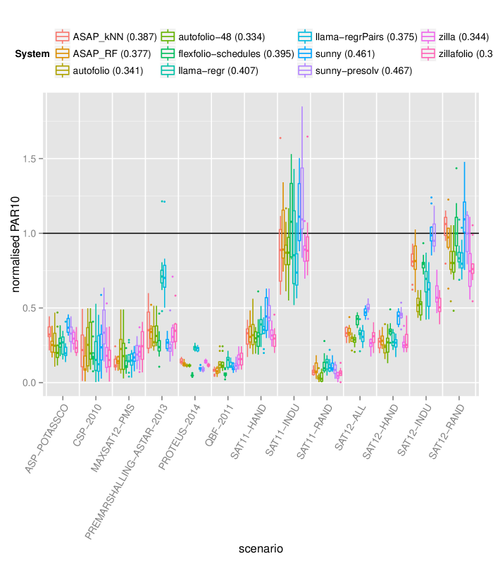
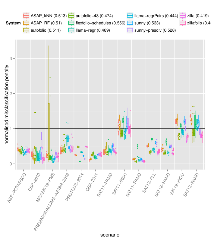
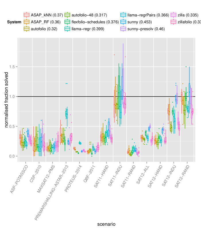
Tables 6 through 8 show the rankings by mean score across all splits and scenarios, but separately for each measure.

	System	Mean PAR10 score
1	autofolio-48	0.33383
2	autofolio	0.34104
3	zilla	0.34414
4	zillafolio	0.34553
5	llama-regrPairs	0.37496
6	ASAP_RF	0.37749
7	ASAP_kNN	0.38658
8	flexfolio-schedules	0.39518
9	llama-regr	0.40749
10	sunny	0.46144
11	sunny-presolv	0.46657

Table 6: Ranking by PAR10.

	System	Mean misclassification penalty
1	zilla	0.41874
2	zillafolio	0.43001
3	llama-regrPairs	0.44447
4	llama-regr	0.46856
5	autofolio-48	0.47449
6	ASAP_RF	0.51015
7	autofolio	0.51131
8	ASAP_kNN	0.51263
9	sunny-presolv	0.52817
10	sunny	0.53324
11	flexfolio-schedules	0.55644

Table 7: Ranking by misclassification penalty.

	System	Mean number of instances solved
1	autofolio-48	0.31668
2	autofolio	0.32015
3	zillafolio	0.33509
4	zilla	0.33522
5	ASAP_RF	0.36045
6	llama-regrPairs	0.36559
7	ASAP_kNN	0.37035
8	flexfolio-schedules	0.37592
9	llama-regr	0.39941
10	sunny	0.45309
11	sunny-presolv	0.45990

Table 8: Ranking by number of instances solved.

Table 9 shows the ranks for the different scenarios for all systems by mean across all measures and splits.

scenario	ASAP_kNN	ASAP_RF	autofolio-48	autofolio	flexfolio-schedules	llama-regr	llama-regrPairs	sunny	sunny-presolv	zilla	zillafolio
ASP-POTASSCO	10	5	2	6	7	3	1	11	9	8	4
CSP-2010	7	1	10	9	6	5	3	8	11	4	2
MAXSAT12-PMS	4	6	10	11	2	3	1	5	8	7	9
PREMARSHALLING-ASTAR-2013	6	4	7	5	2	10	11	3	1	8	9
PROTEUS-2014	5	4	7	6	1	11	10	3	2	9	8
QBF-2011	1	2	9	8	3	6	4	5	7	10	11
SAT11-HAND	3	6	1	7	8	9	5	11	10	4	2
SAT11-INDU	6	8	2	3	10	5	1	9	11	4	7
SAT11-RAND	6	7	1	2	11	10	8	9	5	3	4
SAT12-ALL	7	8	2	3	9	6	5	10	11	1	4
SAT12-HAND	7	8	4	1	9	6	3	10	11	2	5
SAT12-INDU	8	9	1	3	7	6	5	11	10	4	2
SAT12-RAND	10	8	3	4	9	6	5	11	7	1	2

Table 9: Ranks by scenario.

Figures 1 through 3 give a more detailed overview of the performance of the systems on the different scenarios. The colour of each boxplot denotes the system, the mean performance of which is shown in the legend (this corresponds to the number in the respective table above). The boxplot shows the variation of performance across the 10 different splits for each scenario. The solid black line denotes the performance of the single best solver; anything above is worse.

Refer to caption — Figure 1: PAR10 scores.

Two of the SAT scenarios are hard for all systems in the sense that the performance they deliver on at least one of the splits is worse than the performance of the single best solver. For most other scenarios, using any algorithm selection system gives a significant performance improvement compared to the single best solver though.

3.5 Time required to run

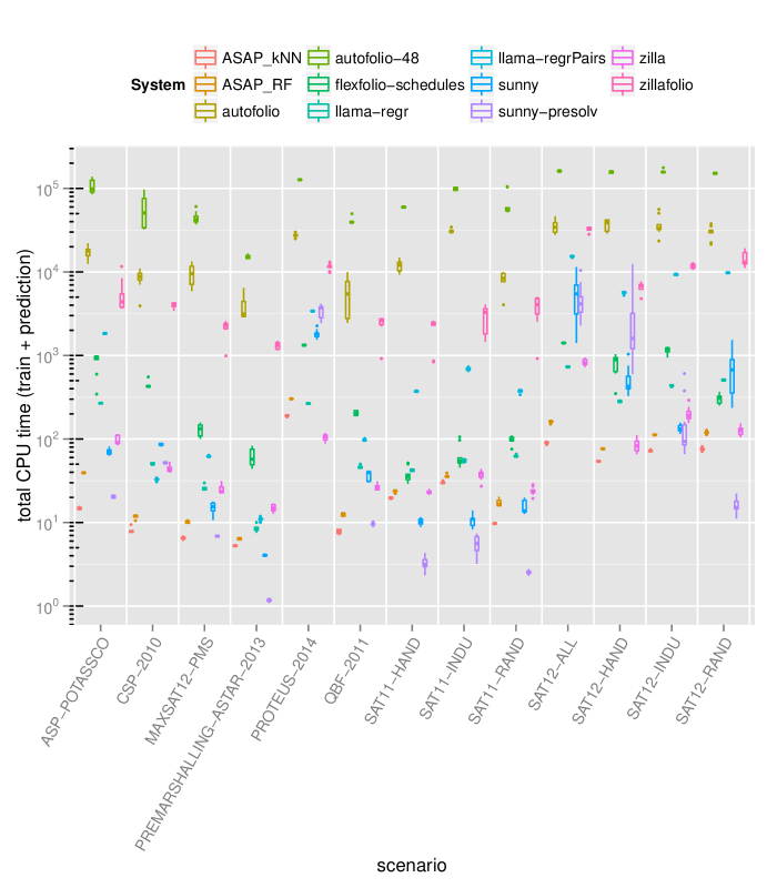
The time required to train the models and make the predictions varied significantly across systems and scenarios, with some completing in minutes and others requiring hours. Figure 4 presents a summary.

4 Acknowledgements

We would like to thank all the participants for taking the time to prepare submissions and their help in getting them to run; in alphabetical order: Alex Fréchette, Chris Cameron, David Bergdoll, Fabio Biselli, Fran¸cois Gonard, Frank Hutter, Holger Hoos, Jacopo Mauro, Kevin Leyton-Brown, Marc Schoenauer, Marius Lindauer, Michèle Sebag, Roberto Amadini, Tong Liu, and Torsten Schaub. We thank Barry Hurley for setting up and maintaining the submission website and Luc De Raedt, Siegfried Nijssen, Benjamin Negrevergne, Behrouz Babaki, Bernd Bischl, and Marius Lindauer for feedback on the design of the challenge.

All data, code and results from the challenge are available at http://4c.ucc.ie/~larsko/downloads/challenge.tar.gz.

Appendix A Llama models used for comparison

A.1 llama-regrPairs

⬇

suppressMessages({

library(optparse)

library(aslib)

library(llama)

library(plyr)

})

ol = list(make_option(c(”-t”, ”–train”), help = ”AS␣scenario␣for␣training”),

make_option(c(”-p”, ”–prediction”), help = ”AS␣scenario␣for␣predictions”))

opts = parse_args(OptionParser(option_list = ol))

suppressWarnings({trainAS = parseASScenario(opts$train)})

suppressWarnings({suppressMessages({ldf = convertToLlama(trainAS)})})

suppressWarnings({testAS = parseASScenario(opts$prediction)})

suppressWarnings({suppressMessages({ldft = convertToLlama(testAS)})})

# some features are removed by the conversion, make sure that we use only the

# intersection

feats = intersect(ldf$features, ldft$features)

ldf$features = feats

ldft$features = feats

tt = trainTest(ldf)

model = regressionPairs(makeLearner(”regr.randomForest”), tt)

preds = model$predictor(ldft$data[,feats])

sched = ddply(preds, c(”id”), function(ss) {

data.frame(instanceID = testAS$feature.values[ss$id[1],”instance_id”],

runID = 1,

solver = ss$algorithm[1],

timeLimit = testAS$desc$algorithm_cutoff_time)

})

write.csv(sched[,c(”instanceID”, ”runID”, ”solver”, ”timeLimit”)], file = stdout(), quote = FALSE, row.names = FALSE)

A.2 llama-regr

⬇

References

- [1] Icon challenge on algorithm selection. http://challenge.icon-fet.eu/. Accessed: 2015-11-12.