Scheduled Relaxation Jacobi method: improvements and applications
Abstract
Elliptic partial differential equations (ePDEs) appear in a wide variety of areas of mathematics, physics and engineering. Typically, ePDEs must be solved numerically, which sets an ever growing demand for efficient and highly parallel algorithms to tackle their computational solution. The Scheduled Relaxation Jacobi (SRJ) is a promising class of methods, atypical for combining simplicity and efficiency, that has been recently introduced for solving linear Poisson-like ePDEs. The SRJ methodology relies on computing the appropriate parameters of a multilevel approach with the goal of minimizing the number of iterations needed to cut down the residuals below specified tolerances. The efficiency in the reduction of the residual increases with the number of levels employed in the algorithm. Applying the original methodology to compute the algorithm parameters with more than 5 levels notably hinders obtaining optimal SRJ schemes, as the mixed (non-linear) algebraic-differential equations from which they result become notably stiff. Here we present a new methodology for obtaining the parameters of SRJ schemes that overcomes the limitations of the original algorithm and provide parameters for SRJ schemes with up to 15 levels and resolutions of up to points per dimension, allowing for acceleration factors larger than several hundreds with respect to the Jacobi method for typical resolutions and, in some high resolution cases, close to 1000. Furthermore, we extend the original algorithm to apply it to certain systems of non-linear ePDEs.
keywords:
Iterative method, Jacobi method, Finite differences method, Elliptic equations.1 Introduction
Partial differential equations (PDEs) are the appropriate mathematical language for modeling many phenomena [1]. In particular, we are interested in elliptic PDEs (ePDEs), that arise when we face the solution of equilibrium problems, in which the time evolution of the system is either neglected or irrelevant. Poisson and Laplace equations are prototype second order ePDEs, with and without source terms respectively.
Though the aforementioned Poisson and Laplace equations posses analytic solutions in a limited number of simple cases, we usually need a numerical solution when more general problems are considered. One of the standard approaches for solving these equations numerically is using finite differences methods. In this approach, both functions and operators are discretized on a numerical mesh, leading to a system of linear algebraic equations, which can be solved with direct or iterative methods. One of the simplest and most studied iterative schemes is the so called Jacobi method [2, 3], whose main drawback is its poor convergence rate.
In oder to improve the efficiency of the Jacobi method, many alternatives have been considered. A popular possibility is the use of preconditioners [4, 5, 6] applied to linear systems, that make the associated Jacobi and Gauss-Seidel methods converge asymptotically faster than the unpreconditioned ones. Indeed, the method we improve on here, can be adapted as a preconditioner for other methods (e.g., the conjugate gradient method). Very widespread is the use of multigrid methods [e.g., 7] that, in many cases, provide the solution with operations, or that can even be employed as preconditioners. Relaxation algorithms [originally introduced in 3], improve the performance of the Jacobi method by considering modifications of the Gauss-Seidel algorithm that include a weight, for instance, successive overrelaxation (SOR) methods [8].
Along this line, [9, YM14 henceforth] have recently presented a significant acceleration (of the order of 100) over the Jacobi algorithm, employing the Scheduled Relaxation Jacobi (SRJ) method. The SRJ method is a generalization of the weighted Jacobi method which adds an overrelaxation factor to the classical Jacobi in a similar fashion to the SOR. This generalization includes a number of different levels, in each of which, the overrelaxation (or underrelaxation) parameter or weight is tuned to achieve a significant reduction of the number of iterations, thus leading to a faster convergence rate. The optimal set of weights depends on the actual discretization of the problem at hand. Although the method greatly improves the convergence rate with respect to the original Jacobi, the schemes presented by YM14, optimal up to and resolutions of up to 512 points per spatial dimension, are still not competitive with other methods used currently in the field (e.g., spectral methods [10], or multigrid methods as commented above). The main advantage of the SRJ method over other alternatives to solve numerically ePDEs is its simplicity and the straightforward parallelization, since SRJ methods preserve the insensitivity of the Jacobi method to domain decomposition (in contrast, e.g., to multigrid methods).
Following basically the same procedure as in YM14, [11, ACCA15 henceforth] has obtained optimal SRJ algorithms with up to levels and multiple numerical resolutions. However, the limitations of the methodology of YM14 to compute optimal parameters for multilevel SRJ schemes prevents to develop algorithms with more than 10 levels. In this paper, we will show a new methodology to evaluate the parameters of optimal SRJ schemes with up to levels and resolutions of up to points per spatial dimension of the problem, which in some cases may yield accelerations of order with respect to the Jacobi method. Considering the difficulty in obtaining the SRJ parameters for , we provide the readers with a comprehensive set of tables for different SRJ schemes and different resolutions.
We begin the paper giving an overview of the SRJ method (Sect. 2) and describing the original methodology for obtaining optimal schemes together with the improvements on them already made in ACCA15 (Sect. 3). Then, we will present in Sect. 3.4, some analytical work which reduces the number of unknowns to solve for to (instead of as in YM14 and ACCA15). In Sect. 4 we show a comparison of the new method to compute optimal parameters for SRJ schemes with that of YM14. Furthermore, we test the SRJ methods in a case study, namely a Poisson equation with Dirichlet boundary conditions (Sect. 5.1) that has analytic solution, and show that optimal SRJ parameters computed for resolutions close to that of the problem at hand can bring two orders of magnitude smaller number of iterations than the Jacobi method to solve such the problem. We have also assessed the performance of the new SRJ schemes with a large number of sublevels with respect to other standard methods to solve ePDEs (Sect. 5.2). In particular, we compare SRJ schemes with and to direct inversion methods and to spectral methods implemented in the LAPACK and LORENE packages, respectively. We outline the most prominent conclusions of our study and discuss the limitations of the current methodology in Sect. 6.
2 SRJ schemes
In this section we recap the most salient results obtained by YM14 and set the notation for the rest of the paper.
First of all, if we define as a single step in a weighted Jacobi iteration using the weight (), then the SRJ method can be cast as a successive application of elementary relaxation steps of the form
where the largest weight, is applied times, and each of the remaining and progressively smaller weights () is applied times, respectively. A single cycle of the scheme ends after elementary steps, where . In order to reach a prescribed tolerance goal, we need to repeat a number times the basic -cycle of the SRJ method. Both, a vector of weights and a vector with the number of times we use each weight, define each optimal scheme. We emphasize that, from the point of view of the implementation, the only difference with the traditional weighted Jacobi is that, instead of having a fixed weight, SRJ schemes of -levels require the computation of weights.
In order to simplify the notation, we define , with and which is in one-to-one correspondence with the previous . Also, we define , where is the fraction of the iteration counts that a given weight is repeated in an -cycle, with .
The basic idea of the SRJ schemes is finding the optimal values for and that minimize the total number of iterations to reach a prescribed tolerance for a given number of points (i.e., numerical resolution) .
3 Finding the optimal parameters
Below we explain how to compute the optimal values of and , following the prescription of YM14 and rewrite some parts of the YM14 algorithm to make them amenable for extension to a larger number of levels and resolutions.
3.1 Converge analysis and optimization problem
We perform a convergence analysis of the method in order to obtain a number of restrictions that the parameters of the SRJ scheme must fulfill. As a model problem, we use the Laplace equation with homogeneous Neumann boundary conditions in two spatial dimensions, in Cartesian coordinates and over a domain with unitary size:
| (1) |
Let us consider a 2nd-order central-difference discretization of Eq. (1) on a uniform grid consisting of zones, and define . Then, we apply the Jacobi method with a relaxation parameter , so that the following iterative scheme results:
| (2) | |||||
| (3) |
where is the index of iteration.
At this point, we perform a von Neumann stability analysis for obtaining the amplification factor,
| (4) |
where is a function of the wave-numbers in each dimension. For the problem at hand,
| (5) |
expresses how much the error can grow up from one iteration to the next one using the relaxation Jacobi method. Thus, if a single relaxation step is performed, we require to ensure convergence. However, in an SRJ scheme, we perform a series of -cycles (Sect. 2). Hence, even if on an elementary step of the algorithm one may violate the condition (which may happen, e.g., if such step is an overrelaxation of the Jacobi method), the condition for convergence shall be obtained for the composition of elementary amplification factors. As we apply Eq. (3) -times but with different weights , the following composition of amplifications factors is obtained:
| (6) |
Finally, it is not important how many times we use each of the weights but their relative frequency of use during an -cycle, which is defined by . Therefore, following YM14, one can define the per-iteration amplification factor function as a geometric mean of the modulus of the cycle amplification factor (Eq. 6):
| (7) |
The previous transformation is very convenient to find deterministic optimal parameters for the SRJ schemes, since it avoids working with a Diophantine equation (Eq. 6), because , while .
From the definition of , it is evident that larger values of the per-iteration amplification factor yield a larger number of iterations for the algorithm to converge. Thus, the optimal values for the SRJ parameters are obtained by looking for the extrema of in , which is the interval bounding the allowed values of , namely
| (8) |
and then, to minimize globally these extrema, so that the error per iteration decreases as much as possible. This sets our optimization problem.
We explicitly point out that the value of depends on the type of boundary conditions of the problem, on the discretization of the elliptic operator and on the dimensionality of the problem. This is not the case for , which equals 2 independent on the boundary conditions, dimensionality and discretization of the elliptic operator. For later reference, we write the explicit form of as a function of the number of dimensions, , for a Cartesian discretization of the elliptic operator an Neumann boundary conditions:
| (9) |
Obviously, we recover Eq. (8) setting . For practical purposes, it is possible to obtain the optimal SRJ parameters for any value of once we know the optimal parameters in 2D. This is done by computing the effective number of points in 2D, , corresponding to a given problem size in -dimensions through the relation:
| (10) |
where the approximated result holds for large values of .
Finally, as stated above, the values of change depending on whether Neumann or Dirichlet boundary conditions are considered, and so the optimal parameters change. Fortunately, there is a simple way to obtain the optimal parameters in case of Dirichlet boundary conditions from the 2D optimal parameters computed for Neumann boundaries, namely
| (11) |
where the approximated result holds when the number of points in each dimension is sufficiently large.
3.2 The non-linear system
In the optimization problem stated in the previous section we need to compute the location of the extrema , hereafter. From the optimization process one must also obtain the rest of the parameters of the SRJ scheme, namely, and . Thus, we need to solve a system to determine all these unknowns.
For the evaluation of , we must take into account that the location of the maxima can be either at the edges of the domain, and (set by Eq. 8), or in other internal values () determined (each of them) by the following condition:
| (12) |
From the solutions of Eq. (12), we obtain the different , which allows us to reduce the number of unknowns of the system from to . Hence, we need to also obtain equations to find a unique solution of the system.
For obtaining the set of the first equations for the system, and following YM14, we equalize all the maxima:
| (13) |
Furthermore, if we assume that , and therefore , a second set of equations can be obtained from the minimization of :
| (14) |
Thereby, our system is now , since the differentiation in Eq. (14) introduces new ancillary variables, namely . The final set of additional equations to account for this extra ancillary variables results from applying the same condition as in Eq. (14) to the remaining values of , deduced from Eqs. (13) and (14):
| (15) |
We note that ACCA15 have shown that setting the optimization problem in terms of as reference variables and considering as function of the later () brings the same numerical solution for the system .
3.3 Basic improvements on the original SRJ algorithm
In order to make the SRJ method competitive with other existing algorithms to solve ePDEs, we must find the optimal parameters of SRJ schemes with a sufficiently large number of levels. Furthermore, since the optimal parameters depend on the resolution of the discretization used to solve a given problem, we also need to compute optimal parameters for a range of numerical resolutions larger than in YM14. In this section we summarize some improvements done in ACCA15, which allow us to solve the system from up to and for resolutions up to . Additional improvements based on analytical results will be commented in the following subsection.
Firstly, the stiffness of increases with the number of levels , which prevented YM14 to compute optimal SRJ schemes for . We have been able to reduce the complexity of the numerical solution by manipulating parts of them algebraically. On the one hand, we have hidden the part of the non-linear system involving the unknowns by solving for them symbolically and using those symbolic placeholders later when solving numerically for and . On the other hand, and after the previous manipulation, we have seen in Sect. 3.2 that we need to solve numerically a non-linear system of equations with the same number of unknowns. We aim to rewrite this system as , which requires obtaining as a function of and . We also compute the solutions of this linear subsystem symbolically. These manipulations of the original system of equations permitted ACCA15 to compute the optimal SRJ parameters for a larger number of levels (up to ) than in YM14.
Secondly, in order to increase the number of points, for the numerical solution of the system, since the accuracy of the results for large values of critically depends on having sufficiently large precision, we needed Mathematica’s ability to perform arbitrary precision arithmetic. We ended up using up to twenty four digits in the representation of the numbers in some cases.
 |
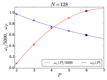 |
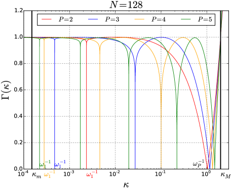
Finally, the non-linear system we have to solve is very sensitive to the initial values that we guess for the unknowns. In ACCA15, we developed a systematic way of setting the initial guesses from the values obtained from lower levels and now we have improved it. As we can see in Fig. 1, when we increase the number of levels , the values of and move towards and , respectively. We can also observe that the inverse of the rest of the weights of a scheme are roughly logarithmically equally spaced between the values and . Hence, we use as approximate location of the initial guesses for the inverse of any weight for an SRJ scheme of levels the following expressions:
| (16) |
when is odd, and
| (17) |
when is even.
Looking at Eqs. (16) and (17), the initial (guess) values of the weights for a new SRJ scheme with an additional level () can be built providing suitable estimates of the smallest and largest weights, which are obtained by fitting to two conics the values of the smallest and largest weights computed for SRJ schemes with to levels, and then extrapolating the result. For instance, in Fig. 1 we show on the right panel the values of and as a function of with red and blue symbols, respectively. If we want to obtain the initial values of and for , we fit the values of and, separately, those of for to a hyperbola or a parabola depending on the flatness of the points, an infer the value for our (in Fig. 1, the fit functions are plot with continuous lines, and the extrapolated values of and for with squares).
As we shall see in the next section, and improving on the procedure outlined in ACCA15, we do not need to provide initial values of , since they can be obtained analytically from the values of .
3.4 Advanced analytical improvements
In this section, we prove two important theorems, which tell us how to calculate analytically the ancillary variables and the parameters of the SRJ schemes in terms of the and variables. Let us start with some technical results we need for the proof of these theorems. Notice that in all products appearing from now on, each index of the product refers only to expressions containing that particular index.
Lemma 1.
Let and be two matrices defined as and , , respectively. The inverse matrices, and , are given by:
| (18) |
| (19) |
Proof.
We just need to check that . For convenience, we define .
We will start checking that
| (20) |
We consider first the case where . In general, taking into account that all the are strictly different, for a polynomial , with , we can do a partial fraction decomposition of the following form:
| (21) |
Considering in the above expression, and evaluating at , we get the desired expression.
We consider now the remaining case . For convenience, we define , that satisfies . For a polynomial , with , we can do a partial fraction decomposition of the following form:
| (22) |
Considering in the above expression, and evaluating at , we get the desired expression.
We use this equality to check the expression for the inverse matrix (as well as below):
| (23) |
Finally, we check the expression for the inverse matrix :
| (24) |
∎
Theorem 1.
| (25) |
Proof.
We have that with are the roots where the local extrema are located. We will also use the already defined . Taking into account the Eqs. (14) and (15), for a fixed value of , we construct the linear system , which in components reads:
| (26) |
where is defined in Lemma 1. We can solve for the ancillary variables , analytically, just inverting the matrix :
| (27) |
Theorem 2.
| (28) |
Proof.
We consider now the equations resulting from Eq. (12) when is replaced by . We write , and obtain:
| (29) |
These equations can be rewritten in matrix form, , which in components reads:
| (30) |
where is defined in Lemma 1. Using Lemma 1 to get the expression of the inverse matrix and doing the corresponding matrix product, we obtain:
| (31) |
In particular, using the simplification proven at the beginning of Lemma 1 for , changing by , and setting just formally, we also get that:
| (32) |
Using this expression,
| (33) |
∎
3.5 Advantages of the rewritten system
In the most general case, as we have commented above, we need to solve a system . With the theorems recently introduced in Sect. 3.4, which basically express as and also as , and substituting them into Eq. (13) and Eq. (14), the non-linear, algebraic-differential system reduces to a purely algebraic system of the form .
We have developed a code that implements everything commented in Sect. 3.3 and that automatically constructs the system and solves it for any value of . This program is written in Mathematica and combines both symbolic with numerical calculations. We obtain two major benefits from the new system of equations to be solved:
-
1.
For any given number of levels , we reduce by orders of magnitude the computing time in the generation of the symbolic system that we need to solve. In ACCA15, we built and needed a lot of time for the symbolic calculations involved in obtaining, on the one hand, , solving the corresponding linear subsystem (Eq. 30) and, on the other hand, . With the new methodology, employing Eqs. (25) and (28), we exchange the role of and , since we have analytic formulae to express the ancillary variables and as functions of and , respectively. With the consequent reduction in the calculation time, the computational time to solve the remaining equations becomes negligible.
-
2.
The solution of the non-linear system to obtain the optimal SRJ parameters needs a suitable methodology to compute their initial values (Sect. 3.3). In ACCA15, we had to provide initial values for and . With the newly derived theorems of the previous section, we only need to provide initial guesses for , since employing Eq. (28) , and satisfies
(34) From the plots of (see, e.g., Fig. 1), we can see that each maximum is roughly placed at:
(35) which are the values that we will use as initial guesses.
With these two improvements, we have reduced by four orders of magnitude the total time for finding the parameters of an optimal scheme. For example, for , it was necessary to spend a calculation time in Mathematica of the order of one week with the methodology employed by ACCA15. In contrast, with the improvements reported here, we can accomplish the same task in tens of seconds. While, in practice, in ACCA15 we were limited (due to the computing time) to SRJ schemes with , now we can tackle larger number of levels.
4 Results
| N | ||||
| 100 | ||||
| 4.15 | 10.12 | 15.86 | ||
| 150 | ||||
| 4.28 | 11.52 | 19.50 | ||
| 200 | ||||
| 4.35 | 12.49 | 22.38 | ||
| 250 | ||||
| 4.39 | 13.21 | 24.75 | ||
| 300 | ||||
| 4.42 | 13.77 | 26.74 | ||
| 350 | ||||
| 4.44 | 14.23 | 28.49 | ||
| 400 | ||||
| 4.46 | 14.62 | 30.12 | ||
| 450 | ||||
| 4.47 | 14.94 | 31.82 | ||
| 500 | ||||
| 4.49 | 15.23 | 32.75 |
| N | ||
|---|---|---|
| 100 | ||
| 20.34 | ||
| 150 | ||
| 26.24 | ||
| 200 | ||
| 31.18 | ||
| 250 | ||
| 35.47 | ||
| 300 | ||
| 39.29 | ||
| 350 | ||
| 42.75 | ||
| 400 | ||
| 45.91 | ||
| 450 | ||
| 48.84 | ||
| 500 | ||
| 51.56 |
In this section we first calibrate our new method comparing the parameters of our optimal SRJ schemes with those of YM14 for (Sect. 4.1). Later (Sect. 4.2), we present new optimal schemes computed employing the new methodology sketched in the previous section, up to .
4.1 Calibration of the method
To calibrate the new methodology, we have recomputed the optimal parameters for SRJ schemes with and found that our results are the same as those obtained by YM14, when we use the same number of points per dimension on the same model problem (Eq. 1).
Following the ideas of YM14, the performance of any SRJ scheme with respect to the Jacobi method can be quantified estimating the convergence performance index, ,
| (36) |
which we have calculated for each SRJ method we have computed, and checked that it approaches its theoretical value when we solve numerically (Eq. 1). We point out that the value of depends on the dimensionality of the problem since the value of does (see, Eq. 9).
YM14 showed that the optimal parameters computed for coarser grids can be used for finer ones. Nevertheless, minimizing the gaps between different values of is important because the acceleration of the convergence with respect to the Jacobi method may not be the largest possible unless we compute the optimal SRJ parameters corresponding to a given problem size. Thus, we have completed the tables presented by YM14 minimizing the possible gaps between resolutions. Furthermore, we have computed the optimal SRJ parameters for a number of intermediate values of in Tab. 1, where we also show the value of .
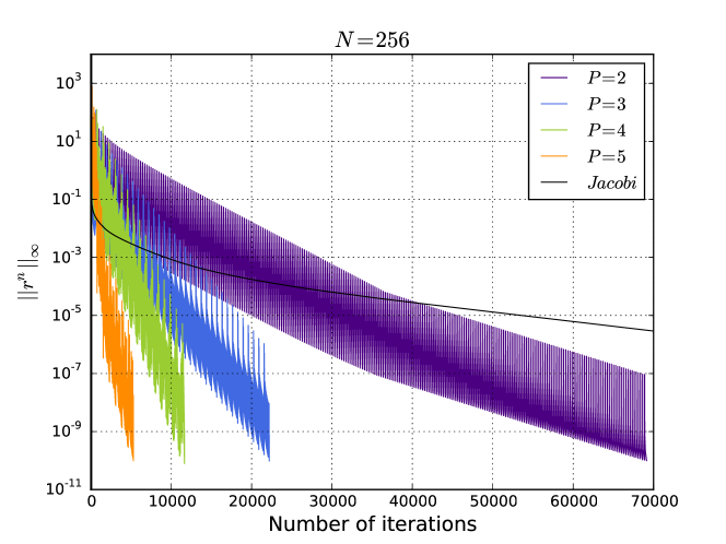
In order to verify the correct behaviour of the schemes computed, we monitor in Fig. 2 the evolution of the difference between two consecutive approximations of the solution for the model problem specified in Eq. (1),
| (37) |
using element-wise norms and operations, that in the bidimensional case would be, for example,
| (38) |
as a function of the number of iterations for SRJ schemes having all the values of given by YM14. In the same figure, we also include the residual evolution for the Jacobi method (black line). As expected, the number of iterations to reach the prescribed tolerance decreases555If not explicitly mentioned, in all the cases considered in this paper the absolute tolerance is fixed so that . as increases. For all the schemes shown in Fig. 2, where the number of points is set to , we have obtained the expected theoretical value of .
| N | Optimal Scheme Parameters | |
| 100 | 35.12 | |
| 150 | 50.34 | |
| 200 | 64.84 | |
| 250 | 78.79 | |
| 300 | 92.3 | |
| 350 | 105.45 | |
| 400 | 118.29 | |
| 450 | 130.87 | |
| 500 | 143.20 | |
| 550 | 155.31 | |
| 600 | 167.24 | |
| 650 | 178.98 | |
| 700 | 190.56 | |
| 750 | 201.99 | |
| 800 | 213.28 | |
| 850 | 224.44 | |
| 900 | 235.47 | |
| 950 | 246.38 | |
| 1000 | 257.19 | |
| 32 | 12.47 | |
| 64 | 23.51 | |
| 128 | 43.75 | |
| 256 | 80.43 | |
| 512 | 146.12 | |
| 262.34 | ||
| 2048 | 465.33 | |
| 4096 | 815.34 | |
| N | Optimal Scheme Parameters | |
| 100 | 35.62 | |
| 150 | 51.31 | |
| 200 | 66.29 | |
| 250 | 80.75 | |
| 300 | 94.79 | |
| 350 | 108.48 | |
| 400 | 121.87 | |
| 450 | 135.00 | |
| 500 | 147.89 | |
| 550 | 160.58 | |
| 600 | 173.08 | |
| 650 | 185.41 | |
| 700 | 197.58 | |
| 750 | 209.60 | |
| 800 | 221.48 | |
| 850 | 233.24 | |
| 900 | 244.87 | |
| 950 | 256.39 | |
| 1000 | 267.81 | |
| 64 | 23.72 | |
| 128 | 44.51 | |
| 256 | 82.46 | |
| 512 | 150.96 | |
| 273.25 | ||
| 489.09 | ||
4.2 New SRJ optimal schemes
After verifying that we recover the optimal parameters computed in YM14, we have improved on their results computing the optimal values of SRJ schemes with . In A we provide the Tables 5 to 12, corresponding to the optimal parameters for SRJ schemes with and various resolutions for the Laplace problem (Eq. 1). In Tables 2, and 3, we show the optimal solution parameters for and .666All the files needed to efficiently implement any of the SRJ algorithms shown in this paper can be found at http://www.uv.es/camap/SRJ.html. We encountered that finding optimal parameters at low resolution is increasingly more difficult as the number of levels increases. Indeed, as we can see, for the minimum value of we have been able to compute is 64. The reason for the inability of the proposed method to find optimal parameters for low and large is that larger values of imply that the results are extremely sensitive to tiny changes in the smaller wave numbers (i.e., to the values of close to ), and small numerical errors prevent a full evaluation of the solution of the non-linear system , unless the (guessed) initial values are very close to the optimal ones.
We remark that thanks to the improvements done (Sect. 3.3) and specially with the analytic solution of a part of the unknowns of the system (Sect. 3.4), not only the optimal solution is achievable, but also it is reachable with a moderate computational cost: employing Mathematica on a standard workstation, the computational time of the optimal parameters ranges from tenths of a second for the scheme to tens of seconds for .
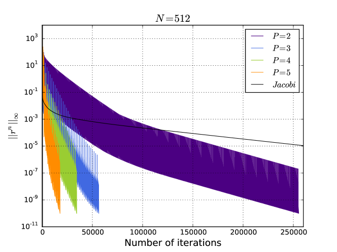
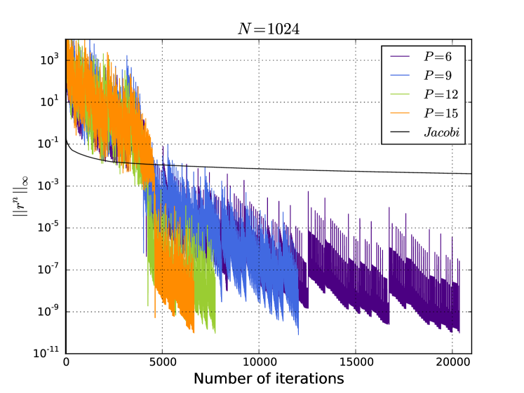
In Fig. 3 we show the evolution of the residual for some of the new optimal SRJ schemes solving the model problem used throughout the paper. These new schemes show a progressively larger efficiency as grows. A good proxy for the performance of the method is the convergence performance index, which grows with the number of levels. We achieve a reduction in the time of computation to solve the problem because of the reduction in the number of iterations to reach convergence. This reduction is roughly proportional to . However, the rate of reduction of the error is non monotonic. For large values of (namely, ), a direct inspection of Fig. 3 shows a faster decline of the residual once any given SRJ method reduces its residual below the one corresponding to the Jacobi method (in this case, this happens after about 4.500 iterations).
4.3 Obtention of the integer parameters
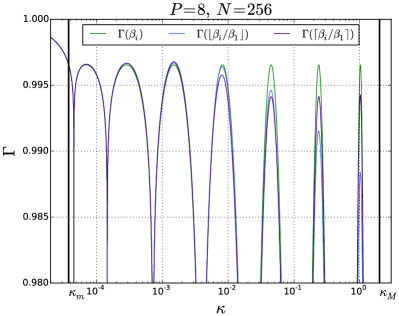
There is a step in the practical implementation of SRJ methods that may impact on the performance of the resulting algorithm, measured by the number of iterations needed to reduce the residual below a prescribed tolerance. Once the solution has been found and we know the real values of and , one must obtain the integer values of . The conversion to integer begins by defining , so that . For the conversion to integer of the rest of the (), we have tested several possibilities, including the floor , rounding to the nearest integer, taking the ceiling function , or combinations of the former alternatives, since it is possible to apply different recipes for every . Each of these alternatives may yield a different number of iterations to reach convergence (see below).
 |
 |
After computing the integer values of , a key point to account for is that the function must remain below 1, since otherwise our method diverges. In Fig. 4 (upper panel) we observe that the amplification factor per -cycle may change by more than 10%, for values of close to , depending on the method adopted to convert to integer.
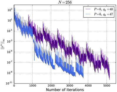
While the number of levels is small, the differences among the distinct conversions from real to integer do not change much either the number of iterations or the convergence rate of the resulting scheme. However, when increases, there can be non-negligible changes in the total number of iterations to reduce the residual of our model equation below a prescribed tolerance. In the lower panel of the Fig. 4 we show the evolution of the residual as a function of the iteration number for two different choices of the integer conversion of into in the case (the optimal parameters of which can be found on Tab. LABEL:table:weiP6_2). We note that there is a difference of more than 1200 iterations () between the distinct integer conversions. Unfortunately, changing the number of levels, the same recipes for converting reals to integers yield efficiencies of the methods that do not display a clear trend. Fortunately, increasing the number of levels by one unit results in a reduction of the number of iterations to reach convergence which is larger than that resulting from any manipulation of the integer values of in an SRJ scheme with a given . Hence, in the following, the results we will provide are obtained by taking simply .
5 Numerical examples
5.1 Poisson equation with Dirichlet boundaries
So far we have considered only the application of SRJ schemes to the solution of the Laplace equation with homogeneous Neumann boundary conditions (Eq. 1). In this section we consider a case study consisting on solving a Poisson equation in two dimensions endowed with Dirichlet boundary conditions. The exact problem setting reads
| (39) | |||||
which has analytic solution:
| (40) |
This kind of problem will help us to assess whether the change in the boundary conditions affects the efficiency of an SRJ scheme. Imposing Dirichlet boundary conditions is typically more challenging than dealing with Neumann ones, since Dirichlet boundary conditions change the value of so that (YM14)
| (41) |
to be compared with Eq. (8). Hence, the optimal SRJ values obtained for a given and Neumann boundary conditions do not exactly coincide with those optimal in problems involving Dirichlet boundaries, hence we must follow the recipe provided in Eq. (11). Furthermore, since in Eq. (5.1) we are considering a Poisson equation, we can test whether the presence of source terms modifies the performance of SRJ methods.
For the case studied we choose a discretization consisting on uniform numerical zones. Although here we do not have Neumann boundary conditions, we will use the optimal values of the SRJ scheme for this case in order to show that even though this choice is not optimal, still it substantially speeds up the solution of the problem with respect to Jacobi. In this case, we have that . If we apply the SRJ scheme with , we must look for the and the parameters in Tab. LABEL:table:weiP10_1. In this case, the table does not provide an entry for , but as YM14 point out, we can chose as (non-optimal) parameters for the SRJ scheme those corresponding to a smaller resolution.777It is, however, possible to compute the optimal values for employing our algorithm. In our case, the closest resolution that matches this criterion in Tab. LABEL:table:weiP10_1 is that corresponding to the row with .
We use the simplest way to obtain the from the ensuring convergence, namely with , resulting in
| (42) |
This means that we will use and once per -cycle, three times per -cycle, etc. In practice, it is necessary to distribute the largest over-relaxation steps over the whole -cycle to prevent the occurrence of overflows. YM14 provide a Matlab script that generates a schedule for the distribution of on the -cycle that guarantees the absence of overflows. We find that an even distribution of the over-relaxations over the entire -cycle is sufficient in order to avoid overflows.
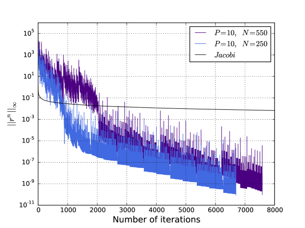
In Fig. 5 we plot the evolution of the residual as a function of the number of iterations for a SRJ scheme with (instead of ), as well as the residual evolution employing the Jacobi method for the solution of Eq. (5.1). This example shows that even picking an SRJ scheme whose parameters are non-optimal for the problem size at hand ( in this case), for the presence of source terms and for the kind of boundary conditions specified (Dirichlet for the problem at hand), we can largely speed up the convergence with respect to the Jacobi method. Theoretically, for the optimal , SRJ method, an acceleration of the order of with respect to the Jacobi method is expected, something confirmed with our numerical results (Fig. 5).
Finally, we briefly illustrate how to find the optimal scheme for Dirichlet boundaries (which are, indeed, the ones with which the problem at hand is set). According to Eq. (11), . Therefore, we choose the row with entry and we proceed as we have done previously. In Fig. 5 we can see that the results are even better than for the (non-optimal) set of parameters with , and Neumann boundary conditions, since in the case with , the accuracy goal is reached with less iterations.
5.2 Poisson equation in spherical coordinates
The Poisson equation appears, among others, in problems involving gravity, either Newtonian or some approximations to General Relativity, and electrostatics. In numerical simulations, e.g., in Astrophysics and Cosmology, the computation of the gravitational potential is usually coupled to a hyperbolic set of equations describing the dynamics of the fluid, e.g., the Euler equations. In those cases the Poisson equation is solved on each time step (or every several time steps) of the evolution of the hyperbolic part. It is thus crucial to test the efficiency of the SRJ compared with other methods currently used by the scientific community. In simulations of stellar interiors, spherical coordinates is a popular choice of coordinates, so we adopt it for our test. To mimic typical astrophysical scenarios we have chosen a test in which the source has compact support and boundary conditions are applied at radial infinity.
The Poisson equation in spherical coordinates reads
| (43) |
being and functions of . For our test we choose the source term to be the series
| (44) |
being the spherical Bessel functions of the first kind and the real part of the spherical harmonics. Only even parity terms, are considered. is the first root of the spherical Bessel function of order , such that . We chose , such that the series is convergent. We impose homogeneous Neumann boundary conditions at , and , and periodic boundary conditions in the direction. If we impose homogeneous Dirichlet condition at radial infinity (), the solution of this elliptic problem is
| (45) |
where the coefficients and can be computed imposing continuity of u and its first derivatives at , resulting in
| (46) |
Since our interest is to assess the performance of the SRJ method under the conditions which are found on real applications, we solve this equation numerically in the domain , and , i.e. only in the region where the sources are non zero, and apply Dirichlet boundary conditions at , using the analytical solution given by Eq. (45).
We emphasize that this problem set up includes boundary conditions of mixed type (Neumann and Dirichlet) and, hence, none of the schemes whose optimal parameters have been tabulated in this paper is strictly optimal. However, as we shall see, even in such conditions, the new schemes presented in this paper with will be competitive with other alternatives in the literature.
We set up three versions of the test with different dimensionality. In the 3D test, we choose and and solve the equation in the domain , and , discretized in an equidistant grid of size points. In the 2D case we consider axisymmetry, i.e., no dependence in and . We choose and and solve in the domain and , discretized in a grid with points. In the 1D case we consider spherical symmetry, i.e. no or dependence in and . We choose , and solve in the domain with points. Since the series in Eqs. (44) and (45) are convergent, we compute them numerically by adding terms until the last significant digit does not change. We use a second order finite difference discretization for Eq. (43) and one ghost cell in each direction to impose boundary conditions. For convenience, we multiply Eq. (43) by in the discretized version.
As an example, we present explicitly the discretization of the 1D problem. The 2D and 3D discretizations are analogous to what is described here. We use a staggered grid with ghost cells, with , where . Points and are ghost cells used only for the purpose of imposing boundary conditions. Using second order centered derivatives and imposing spherical symmetry () Eq. (43), multiplied by , can be discretized as
| (47) |
where sub-index indicates a function evaluated at . By imposing boundary conditions it is possible to set the values of and . The resulting linear system of equations with unknowns, , can be written in matrix form
| (48) |
being the elements of the coefficient matrix, which in the 1D case is a tridiagonal matrix
| (49) |
Note that this matrix is diagonally dominant by rows and columns except for the first two rows and the first column. If the factor were not present, the matrix would not be diagonally dominant by columns and the convergence of the iterative methods could not be guaranteed. Once the boundary conditions are applied, the coefficient matrix is effectively modified. Wether the resulting effective matrix is diagonally dominant or not depends crucially on how the boundary conditions are applied.
We impose Dirichlet boundary conditions at the outer boundary by setting , being the analytic solution that given by Eq. (45). In this case the equation at results
| (50) |
being an extension of the coefficient matrix used for practical purposes. At the inner boundary we impose homogeneous Neumann conditions, i.e. . A second order discretization of this boundary condition is not unique. Two possible discretizations are of the boundary condition are
| (51) | |||||
| (52) |
Naively, one would expect that imposing either or , would be an appropriate boundary condition. However, either of these cases results in an effective coefficient matrix which is not diagonally dominant. To cure this pathology we impose , which is compatible with both discretizations of the boundary condition. Since we are fixing not only the value of the ghost cell, , but also the value , this condition reduces the dimensionality of the linear system by . The resulting effective coefficient matrix is a tridiagonal matrix of size , with indices . The elements read
| (53) |
The new matrix is diagonally dominant by rows and columns, which guarantees the convergence of Jacobi-based iterative methods.
In practice, the effective coefficient matrix, , is not used in the iterative methods directly. Instead we use a coefficient matrix extended to the ghost cells and we set at each iteration the values at the ghost cells ( and ) and at according to prescription given above. This procedure is equivalent to using the effective coefficient matrix, but it eases the implementation of the algorithm.
We perform series of calculations for different values of the number of points . For each calculation we use the SRJ coefficients computed in the previous sections matching the corresponding value of . For each series we perform calculations using coefficients computed with different values of . The tolerance goal is set to , which depends on the number of points. Since we use a second order discretization, this scaling in the tolerance ensures that the difference between the numerical and the analytical solution is dominated by finite differencing errors and at the same time avoids unnecessary iterations in the low resolution calculations. This prescription for the tolerance mimics the tolerance choice that is used under realistic conditions and renders a fairer comparison in the computational cost between different resolutions. For comparison we also perform calculations using other iterative methods: Jacobi, Gauss-Seidel and SOR (weight equal to ). For each case involving iterative methods we perform two calculations: the ab initio calculation in which the solution is initialized to zero, and the realistic calculation in which the solution is initialized to , being a random number in the interval . The realistic calculation tries to mimic the conditions encountered in many numerical simulations in which an elliptic equation (or a system of PDEs) is solved coupled with evolutionary (hyperbolic) PDEs,888For instance, this is the case of the fluid equations. which are typically solved using explicit methods, whose time step is limited by the Courant-Friedrichs-Lewy (CFL) condition. This means that the change in the source of the Poisson equation between subsequent calculations is ; therefore, if the solution of the previous time step is used for the iteration in the elliptic solver, this should differ only , from the solution.
In addition to iterative methods, we perform the calculations using a direct inversion method and spectral methods. In the direct inversion method, we compute the LU factorization of the matrix associated with the coefficients of the discretized version of the equation by performing Gaussian elimination using partial pivoting with row interchanges. We use the implementation in the dgbtrf routine of the LAPACK library [12], which allows for efficient storage of the matrix coefficient in bands. Once the LU decomposition is known, we solve the system of linear equations using the dgbtrs routine. Since this method is non-iterative, its computational cost does not depend on the initial value. However, this approach has advantages when used repeatedly, coupled to evolution equations (e.g., for a fluid). Most of the computational cost of this method is due to the LU decomposition, but once it has been performed, solving the linear system for different values of the sources is computationally less intensive. Therefore, we consider the computational cost of the whole process, LU decomposition and solution of the system, in the ab initio calculations, while only the solution of the linear system, assuming the LU decomposition is given, in the realistic calculations.
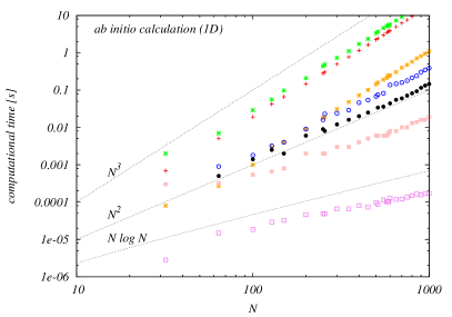
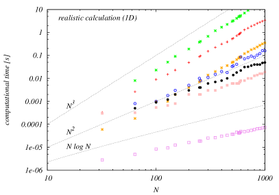
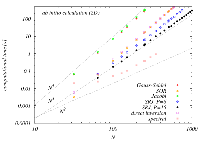
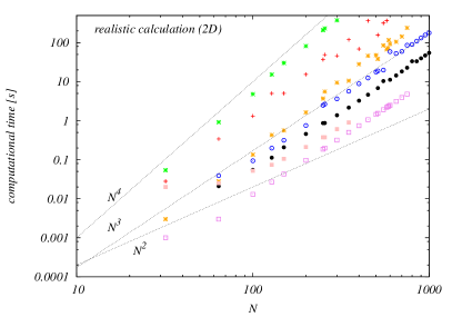
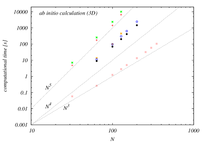
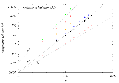
For the spectral solver we use the LORENE library [13]. To provide results that are comparable to all other numerical methods used in the present work we use the following procedure: first we evaluate the source, , at the finite differences grid used in all other numerical methods; then, the source is interpolated to the collocation points in the spectral grid, which do not coincide with the finite differences grid; next the solution is computed by means of the LORENE library; finally the function is evaluated at the cells of the finite differences grid. The details of the procedure are described in [14]. The accuracy of the numerical method is dominated by the second order finite differences discretization error associated with the finite differences grid, provided sufficient number of collocation points are used in the spectral grid. We have tested that it is sufficient to use collocation points per dimension to fulfill this requirement. When using the spectral solver, there is no difference in the computational cost in ab initio or realistic calculations.
We have performed the calculations using a 3.4 GHz Intel core i7 and 16 GB of memory. All codes and libraries have been compiled using the GCC compiler [15]. We have measured the computational time for each method timing exclusively the part of the code involved in the computation and not the allocation and initialization of variables. Figure 6 shows the dependence of the computational time for 1D, 2D and 3D tests in the ab initio calculations and the realistic calculations setups. As expected, for any dimensionality, the SRJ methods render a significant speed up with respect to other iterative methods, due to the smaller number of iterations needed. Only SOR method has comparable computational time for low resolutions (). The computational time for SRJ methods scales approximately as , being the dimensionality of the test, i.e. the number of iterations is proportional to . In comparison, the computational cost of other iterative methods (Jacobi, Gauss-Seidel, SOR), scale approximately as , i.e. the number of iterations needed scales as . This factor improvement of SRJ with respect other iterative methods ensures that the method will always be less costly for sufficient high resolution. Compared to non-iterative methods the results depend on the dimensionality of the test.
For the 1D test, both spectral and the direct inversion method are significantly faster than SRJ. The computational cost of both methods are close to . Therefore, we conclude that SRJ methods are not competitive for 1D problems, even when realistic conditions are considered.
In 2D, the computational cost of the direct inversion method for ab initio calculations increases significantly, scaling as , because the associated matrix is not tridiagonal anymore, as in the 1D case, but is a banded matrix of band size . Hence, the direct inversion method is more costly than SRJ for resolutions . However, in the realistic calculation, in which the LU decomposition is not performed, the direct inversion method is still the fastest, with a computational time scaling as (the same as SRJ) but with lower computational cost. Due to limitations of the LORENE library, we were not able to perform multidimensional computations using spectral methods for . Compared to , spectral methods are about a factor faster than SRJ in realistic calculations and become comparable for . It seems fair to say that spectral methods perform better for ab initio calculations, since in this case, SRJ methods (see and in Figure 6) scale as . Therefore, we conclude that for 2D calculations SRJ is a competitive method, when compared with spectral methods. Although the direct inversion method is the fastest in the range of values of selected for our tests, we expect that this advantage will disappear when going to larger number of points; the memory needed for the direct inversion method scales as (due to the explicit use of the banded structure of the matrix) in comparison with of all other methods (iterative and spectral). This strongly limits the size of the problem to be solved without using parallelization.
In 3D all computations are significantly more costly, so we limit our tests to what is achievable within hour of computation time. For the SRJ methods tested this is . For the computational cost of spectral methods is a factor lower than a SRJ method with , in the realistic calculation. Using the SRJ parameters for and an effective number of points per dimension as given by Eq. (10), the SRJ method becomes faster, so that it is “only” slower than the spectral method. The conclusion is that spectral methods still seem to have advantages over SRJ methods, for the 3D test presented. However, both spectral and SRJ methods scale approximately as in 3D. Due to the large amount of memory needed for the direct inversion method, which scales as , we did not present any such calculation for the 3D case. In practice, this limitation makes the direct inversion method unfeasible for computations in a single CPU. The performance of all these methods and a comparison between them in a parallel architecture is beyond the scope of this work.
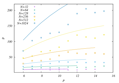
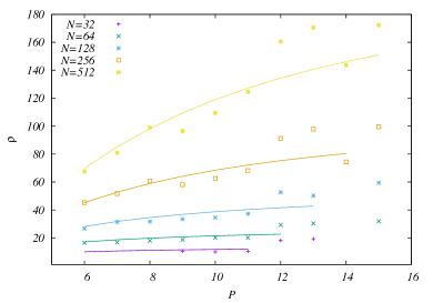
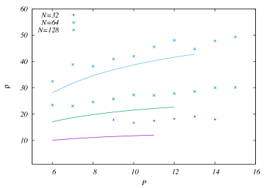
Finally we have estimated numerically the value of for different SRJ weights, to be compared with the theoretical predictions. For this purpose we compute the ratio of number of iterations needed with Jacobi and a given SRJ method, using the same tolerance and resolution, . Left panels of Fig. 7 show the dependence of on for several values of , computed using the set of ab initio calculations. Regardless of the dimensionality, in all calculations the numerical values of are close to the theoretical predictions (solid lines). In the 1D test problems there is a tendency of the theoretical values to overestimate the numerically computed value. This trend is exacerbated for large values of (namely, ). In 3D the situation is reversed, and the theoretical value of falls below the numerical one. To explain these differences, we shall consider that the optimal weights depend on the dimensionality of the problem, since does also depend on dimensionality (see Eq. 9). As the optimization of the weights has been performed for the 2D case, it is not surprising to find such discrepancies when using the same weights and the same value of in a problem with different dimensionality. Indeed, we have repeated some of the 3D and 1D test problems employing the optimal SRJ parameters corresponding to the effective number of points set according to Eq. (10), and found that (i) the SRJ scheme runs is less iterations and, (ii) for this effective number of points, the theoretical convergence performance index, computed with the dimensionality corrections mentioned below Eq. (36), becomes an upper bound for the numerical values of . Adding to this arguments, we also note that the discretization of the Laplacian operator in spherical coordinates may also change slightly the optimal weights. Finally, another factor that explains the discrepancies is that the boundary conditions of this problem are mixed (as commented above), and the optimal weights are computed for purely Neumann boundaries.
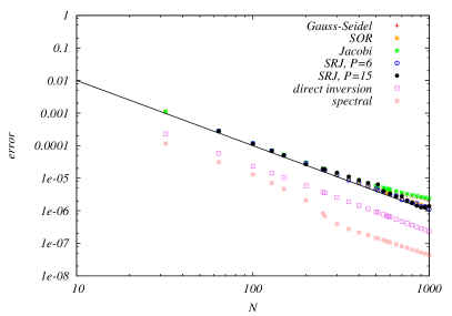
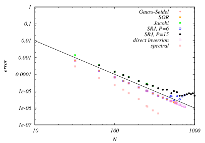
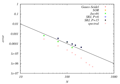
The right panels of Fig. 7 show the error in the solution as a function of , computed as the -norm of the difference between the numerical and the analytical solution. In all cases the error is dominated by the finite difference error associated to the discretization of the elliptic operator, which, for a second order method, is expected to be . This is a symptom that our prescription for the tolerance is yielding converged numerical solutions, in iterative methods. It also shows that the number of spectral grid points used is sufficient for such calculations.
We have also tried different discretizations of the equation and the boundary conditions, although not as systematically as the presented case. In general, using discretizations which lead to non-diagonally dominant coefficient matrices, increases the number of iterations to converge or, in some cases, they do not converge at all. The Jacobi method is the most sensitive to this, while all other iterative methods (Gauss-Seidel, SOR, SRJ) seem less affected by this issue. As an example, if just is used for the inner boundary condition (consistent with Eq. (51)), the Jacobi method needs about times more iterations in 1D, while all other iterative methods remain almost unaltered (only SOR shows differences for ). This is an indication that the new method is not only faster than well-known iterative methods but can also be more robust than some of them.
5.3 Grad-Shafranov equation in spherical coordinates
The Grad-Shafranov (GS) equation [16, 17] describes equilibrium solutions in ideal magnetohydrodynamics for a two dimensional plasma. It is of interest in studying the plasma in magnetic confinement fusion (e.g. Tokamaks), the solar corona and neutron star magnetospheres, among others.
In spherical coordinates the magnetic field of an axisymmetric () plasma configuration can be expressed as
| (54) |
where is the vector potential and is the unit vector in the direction. The flux function, , is constant along magnetic field lines and is a measure of the poloidal magnetic field strength. The toroidal function, , is a measure of the toroidal field strength. Using Ampere’s law, , being the electric current, the flux function can be linked to the toroidal current as
| (55) |
where is the GS elliptic operator. For simplicity we consider here the case in which the inertia of the fluid can be neglected (magnetically dominated). In this case, if we impose force balance, , the toroidal function depends on the flux function, . As a result Eq. (55) leads to the GS equation
| (56) |
Not neglecting the inertia of the fluid leads to additional pressure terms, which are not considered here. A popular choice for the toroidal function is , being a constant. In this case the GS equation results in
| (57) |
which is a suitable elliptic problem to be solved with SRJ methods. Equation (57) resembles the Helmholtz differential equation in that it contains a Laplacian-like operator and a linear term in . Therefore, this test will show the ability of SRJ methods to handle more complicated elliptic operators. In addition we use this test to demonstrate the ability of iterative methods to handle boundary conditions imposed at arbitrarily shaped boundaries.
We compute the solution of Eq. (57) for two sets of boundary conditions, in the numerical domain and . In all cases we impose homogeneous Dirichlet conditions at and . In test A we impose Dirichlet boundary conditions at and with . In the case , the solution for this test is a dipolar field. As the value of is increased the solution results in a twisted dipole.
In test B we solve the GS equation in part of the domain, the region defined by
| (58) |
inside the aforementioned numerical domain. The boundary of this region intersects the sphere at and . At we impose Dirichlet boundary conditions with , and homogeneous Dirichlet conditions at the remaining boundaries. Imposing boundary conditions in arbitrarily shaped boundaries is straightforward when using iterative methods such as SRJ; we set everywhere outside the region (58) and apply the SRJ iteration only inside this region using a mask.
| test A | test B | ||||
|---|---|---|---|---|---|
| iterations | computational | iterations | computational | ||
| time [s] | time [s] | ||||
| 0 | 5350 | 8.55 | 0 | 3450 | 1.78 |
| 0.01 | 5350 | 8.55 | 0.01 | 3450 | 1.78 |
| 0.1 | 5350 | 8.58 | 0.1 | 3450 | 1.78 |
| 0.2 | 4660 | 7.48 | 0.5 | 3600 | 1.86 |
| 0.3 | 7750 | 12.43 | 1.0 | 3550 | 1.84 |
| 0.31 | 9830 | 15.73 | 1.3 | 3410 | 1.78 |
| 0.32 | 13540 | 21.80 | 1.4 | 3660 | 2.41 |
| 0.33 | 21390 | 34.38 | 1.45 | 4980 | 2.57 |
| 0.34 | 49080 | 79.22 | 1.47 | 11620 | 6.03 |
In both tests we use a second order discretization of the GS equation and a numerical resolution of equispaced grid points covering the numerical domain. We solve the equations using the SRJ method with weights corresponding to and . In both tests we initialize to zero in the whole domain. Table 4 shows the number of iterations and computational time to obtain a numerical solution with residual bellow , depending on the value of used.
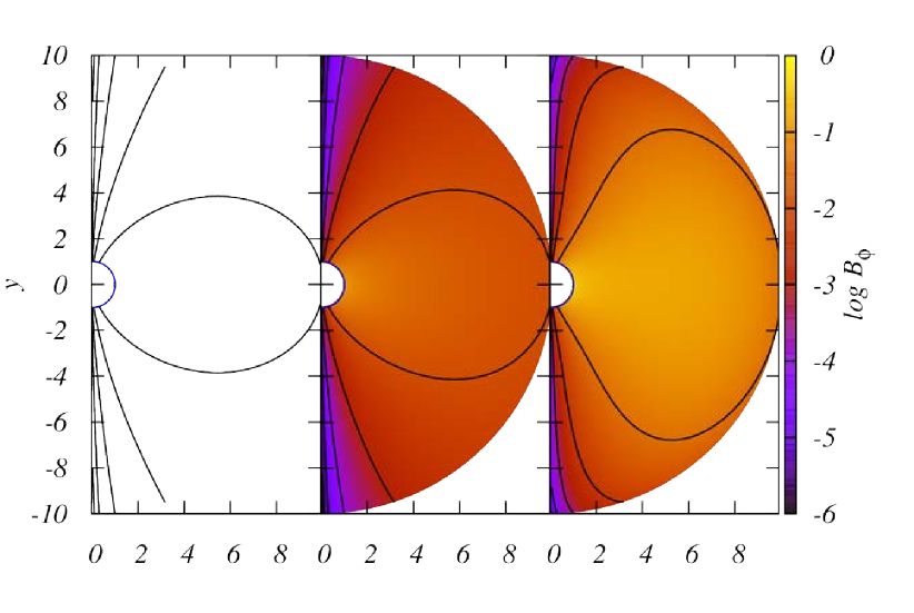
Upper panels of Fig. (8) show the results for test A, for three different values of . For the case , the analytical solution is . In this case the maximum difference between the analytical and the numerical result, in absolute value, is , which is consistent with the second order discretization (). For a toroidal component appears, but the flux function, , remains essentially the same. For higher values of there is a tendency of the magnetic field lines to become more inflated, to support the increased magnetic tension due to the high magnetic field. In this regime the number of iterations needed in the SRJ method increases. We were not able to obtain solutions for values larger than . This is not a problem of the numerical method itself, since other methods (Jacobi, Gauss-Seidel, SOR) show similar behavior. The value corresponds to an eigenvalue of the GS operator. For this case the matrix associated to the discretization of the GS equation is singular and hence it cannot be inverted. This is causing the convergence problems near this point.
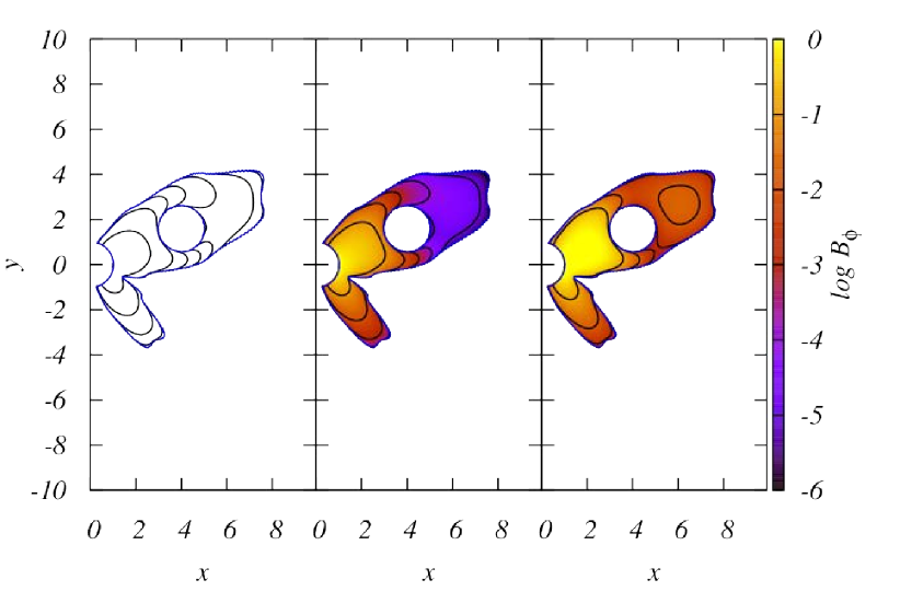
Lower panels of Fig. (8) show the results for test B, for three different values of . This case behaves qualitatively similar to test A but with more complicated geometry. The case shows no toroidal field, which appears as is increased. For the flux function is still similar to that of the untwisted case, albeit slightly deformed. For , the maximum value that we were able to achieve, the topology of the field has changed, showing a region of close magnetic field lines in the upper right part of the domain. As in test A, the difficulty to achieve convergence for larger values of is related to the presence of an eigenvalue of the GS operator. Note that the solution is everywhere smooth, and magnetic field lines (black lines) are tangent to the domain boundary (blue curve) as expected (except for where non-zero Dirichlet boundary conditions are applied).
In general the SRJ method shows reasonable rates of convergence and computational time to solve the problem with high accuracy, despite of the complicated boundary conditions. This renders a method which can be used in real applications of the GS equation with a good trade of excellent performance and ease of implementation.
6 Conclusions and future work
Building upon the results of YM14, we have devised a new method for obtaining the optimal parameters for SRJ schemes applied to the numerical solution of ePDEs.
We have shown that the new multilevel SRJ schemes keep improving the convergence performance index of the scheme, which means that increasing the value of we obtain ever larger acceleration factors with respect to the Jacobi method. In the present paper we report acceleration factors of a few hundreds and, in some cases, more than 1000 with respect to the Jacobi method if a sufficiently large number of points per dimension (namely, ) and number of levels are considered.
Mainly due to the fact that we have derived analytic solutions for part of the unknowns, our new method reduces the stiffness of the non-linear system of equations from which optimal parameters are computed, allowing us to obtain new SRJ methods for up to and arbitrarily large number of points per dimension .
From this number of levels, new problems arise, which hinder the computation of optimal coefficients at relatively low number of discretization points. These problems are related to the fact that for large values of the solution to the problem are very sensitive to tiny changes in the smaller wave numbers, and small numerical errors prevent the succesful evaluation of the solution of even the simplified system of non-linear equations resulting from the algebraic simplifications we have shown here. In order to tackle this problem, we are working in two new improvements: an alternative equivalent new system, and alternative methods for the solution of the optimization problem (including genetic algorithms).
Currently, we have reached acceleration factors that have made that the SRJ methods become competitive (depending on the dimensionality of the problem and its size) with, e.g., spectral methods for the solution of some ePDEs. In particular, we have made the comparison in the case of an astrophysical problem that we are interested in for whose solution we were using spectral methods. We find that for 1D Poisson-like problems, the fastest method of solution is the direct inversion method implemented in LAPACK. This happens because the LU decomposition of the matrix solver, where most of the computational work is done, needs to be performed once, and the it can be stored for the rest of the evolution. In 2D, the best performing method depends on whether our initial guess is close to the actual solution or far off. In realistic applications, where ePDEs are coupled to systems of hyperbolic PDEs, the solution from a previous time iteration does not change significantly over the course fo a single timestep. In such conditions, the LAPACK libraries are the best performing. However, spectral methods are advantageous if, in 2D, the initial values are far from the actual solution of the problem. We further note that in realistic coupled systems, and for a relatively large number of points per dimension (), the SRJ methods are competitive with spectral ones. In 3D applications, we find that the total computational cost of SRJ methods scales in 3D as , i.e, as in the case of spectral methods. Considering that (i) applying direct inversion methods to 3D problems is unfeasible because of memory restrictions, and that (ii) SRJ methods can be parallelized straightforwardly (much more easily than, e.g., spectral or multigrid methods), we foresee that they are a competitive alternative for the solution of elliptic problems in supercomputing applications and in 3D. We are studying improvements in the method from this point of view. Finally, we outline that the easy implementation of complex boundary conditions in SRJ methods is also an advantage with respect to other existing alternatives.
Acknowledgements
We thank P. Mimica for bringing the paper YM14 to our attention. We acknowledge the support from the European Research Council (Starting Independent Researcher Grant CAMAP-259276), and the partial support of grants AYA2013-40979-P, PROMETEO-II-2014-069 and SAF2013-49284-EXP. We thankfully acknowledge the computer resources, technical expertise and assistance provided by the Servei de Informàtica of the University of Valencia.
Appendix A Compendium of parameters of optimal SRJ schemes
| N | Optimal Scheme Parameters | |
| 100 | 23.75 | |
| 150 | 31.57 | |
| 200 | 38.38 | |
| 250 | 44.49 | |
| 300 | 50.06 | |
| 350 | 55.22 | |
| 400 | 60.04 | |
| 450 | 64.57 | |
| 500 | 68.86 | |
| 550 | 72.94 | |
| 600 | 76.82 | |
| 650 | 80.55 | |
| 700 | 84.12 | |
| 750 | 87.56 | |
| 800 | 90.88 | |
| 850 | 94.09 | |
| 900 | 97.20 | |
| 950 | 100.21 | |
| 1000 | 103.13 | |
| 10.08 | ||
| 17.15 | ||
| 28.28 | ||
| 45.18 | ||
| 512 | 69.86 | |
| 104.5 | ||
| 2048 | 151.3 | |
| 4096 | 211.8 | |
| 8192 | 287.3 | |
| 16384 | 377.6 | |
| 481.6 | ||
| N | Optimal Scheme Parameters | |
| 100 | 26.38 | |
| 150 | 35.79 | |
| 200 | 44.19 | |
| 250 | 51.87 | |
| 300 | 59.01 | |
| 350 | 65.71 | |
| 400 | 72.05 | |
| 450 | 78.08 | |
| 500 | 83.85 | |
| 550 | 89.38 | |
| 600 | 94.70 | |
| 650 | 99.84 | |
| 700 | 104.8 | |
| 750 | 109.6 | |
| 800 | 114.3 | |
| 850 | 118.9 | |
| 900 | 123.3 | |
| 950 | 127.6 | |
| 1000 | 131.9 | |
| 10.68 | ||
| 64 | 18.67 | |
| 128 | 31.80 | |
| 256 | 52.76 | |
| 512 | 85.20 | |
| 133.8 | ||
| 2048 | 204.5 | |
| 4096 | 303.8 | |
| 8192 | 438.7 | |
| 16384 | 616.2 | |
| 842.0 | ||
| N | Optimal Scheme Parameters | |
| 100 | 28.46 | |
| 150 | 39.17 | |
| 200 | 48.90 | |
| 250 | 57.94 | |
| 300 | 66.43 | |
| 350 | 74.48 | |
| 400 | 82.16 | |
| 450 | 89.53 | |
| 500 | 96.62 | |
| 550 | 103.5 | |
| 600 | 110.1 | |
| 650 | 116.5 | |
| 700 | 122.8 | |
| 750 | 128.9 | |
| 800 | 134.9 | |
| 850 | 140.7 | |
| 900 | 146.4 | |
| 950 | 151.9 | |
| 1000 | 157.4 | |
| 11.14 | ||
| 64 | 19.84 | |
| 128 | 34.60 | |
| 256 | 58.98 | |
| 512 | 98.21 | |
| 160.0 | ||
| 2048 | 254.3 | |
| 4096 | 394.6 | |
| 8192 | 438.7 | |
| 16384 | 882.9 | |
| 1273 | ||
| N | Optimal Scheme Parameters | |
| 100 | 30.12 | |
| 150 | 41.92 | |
| 200 | 52.78 | |
| 250 | 62.97 | |
| 300 | 72.62 | |
| 350 | 81.84 | |
| 400 | 90.69 | |
| 450 | 99.23 | |
| 500 | 107.49 | |
| 550 | 115.52 | |
| 600 | 123.32 | |
| 650 | 130.93 | |
| 700 | 138.35 | |
| 750 | 145.61 | |
| 800 | 152.72 | |
| 850 | 159.69 | |
| 900 | 166.53 | |
| 950 | 173.24 | |
| 1000 | 179.84 | |
| 11.50 | ||
| 64 | 20.78 | |
| 128 | 36.87 | |
| 256 | 64.15 | |
| 512 | 109.44 | |
| 182.96 | ||
| 2048 | 299.64 | |
| 4096 | 480.54 | |
| 8192 | 754.47 | |
| N | Optimal Scheme Parameters | |
| 100 | 31.49 | |
| 150 | 44.20 | |
| 200 | 56.02 | |
| 250 | 67.18 | |
| 300 | 77.83 | |
| 350 | 88.06 | |
| 400 | 97.94 | |
| 450 | 107.50 | |
| 500 | 116.80 | |
| 550 | 125.85 | |
| 600 | 134.69 | |
| 650 | 143.33 | |
| 700 | 151.80 | |
| 750 | 160.09 | |
| 800 | 168.23 | |
| 850 | 176.23 | |
| 900 | 184.10 | |
| 950 | 191.84 | |
| 1000 | 199.47 | |
| 11.78 | ||
| 64 | 21.54 | |
| 128 | 38.74 | |
| 256 | 68.49 | |
| 512 | 118.99 | |
| 203.09 | ||
| 2048 | 340.42 | |
| 4096 | 560.18 | |
| 8192 | 904.73 | |
| N | Optimal Scheme Parameters | |
| 100 | 32.64 | |
| 150 | 46.12 | |
| 200 | 58.75 | |
| 250 | 70.76 | |
| 300 | 82.28 | |
| 350 | 93.38 | |
| 400 | 104.15 | |
| 450 | 114.61 | |
| 500 | 124.81 | |
| 550 | 134.77 | |
| 600 | 144.52 | |
| 650 | 154.08 | |
| 700 | 163.46 | |
| 750 | 172.68 | |
| 800 | 181.75 | |
| 850 | 190.67 | |
| 900 | 199.47 | |
| 950 | 208.14 | |
| 1000 | 216.69 | |
| 32 | 12.02 | |
| 64 | 22.17 | |
| 128 | 40.31 | |
| 256 | 72.17 | |
| 512 | 127.22 | |
| 220.76 | ||
| 2048 | 376.94 | |
| 4096 | 633.15 | |
| N | Optimal Scheme Parameters | |
| 100 | 33.60 | |
| 150 | 47.75 | |
| 200 | 61.09 | |
| 250 | 73.83 | |
| 300 | 86.10 | |
| 350 | 97.97 | |
| 400 | 109.52 | |
| 450 | 120.77 | |
| 500 | 131.77 | |
| 550 | 142.53 | |
| 600 | 153.09 | |
| 650 | 163.47 | |
| 700 | 173.67 | |
| 750 | 183.70 | |
| 800 | 193.59 | |
| 850 | 203.34 | |
| 900 | 212.97 | |
| 950 | 222.47 | |
| 1000 | 231.85 | |
| 32 | 12.22 | |
| 64 | 22.71 | |
| 128 | 41.64 | |
| 256 | 75.32 | |
| 512 | 134.37 | |
| 236.32 | ||
| 2048 | 409.64 | |
| 4096 | 699.67 | |
| N | Optimal Scheme Parameters | |
| 100 | 34.43 | |
| 150 | 49.15 | |
| 200 | 63.10 | |
| 250 | 76.48 | |
| 300 | 89.41 | |
| 350 | 101.97 | |
| 400 | 114.20 | |
| 450 | 126.15 | |
| 500 | 137.85 | |
| 550 | 149.33 | |
| 600 | 160.61 | |
| 650 | 171.71 | |
| 700 | 182.64 | |
| 750 | 193.41 | |
| 800 | 204.03 | |
| 850 | 214.53 | |
| 900 | 224.89 | |
| 950 | 235.13 | |
| 1000 | 245.27 | |
| 32 | 12.38 | |
| 64 | 23.16 | |
| 128 | 42.78 | |
| 256 | 78.06 | |
| 512 | 140.62 | |
| 250.09 | ||
| 2048 | 438.96 | |
| 4096 | 760.22 | |
References
-
[1]
L. Evans, Partial
Differential Equations (Graduate Studies in Mathematics), American
Mathematical Society. 2nd edition. ebenda, 2010.
URL http://books.google.es/books?id=TwFInwEACAAJ - [2] C. Jacobi, Ueber eine neue auflösungsart der bei der methode der kleinsten quadrate vorkommenden linären gleichungen, Astronomische Nachrichten 22 (20) (1845) 297 – 306. doi:10.1002/asna.18450222002.
- [3] L. F. Richardson, The Approximate Arithmetical Solution by Finite Differences of Physical Problems Involving Differential Equations, with an Application to the Stresses in a Masonry Dam, Royal Society of London Philosophical Transactions Series A 210 (1911) 307–357. doi:10.1098/rsta.1911.0009.
- [4] M. L. Juncosa, T. W. Mulliken, On the increase of convergence rates of relaxation procedures for elliptic partial differential equations, J. Assoc. Comput. Math. 7 (1960) 29–36.
- [5] A. D. Gunawardena, S. K. Jain, L. Snyder, Modified iterative methods for consistent linear systems, Linear Algebra and its Applications 154 (1991) 123–143. doi:http://dx.doi.org/10.1016/0024-3795(91)90376-8.
- [6] D. Noutsos, M. Tzoumas, On optimal improvements of classical iterative schemes for Z-matrices, Journal of Computational and Applied Mathematics 188 (2006) 89–106.
- [7] U. Trottenberg, C. W. Oosterlee, A. Schüller, Multigrid, Academic Press, 2001.
- [8] D. Young, Iterative methods for solving partial difference equations of elliptic type, Trans. Amer. Math. Soc. 76 (1954) 92–111.
-
[9]
X. I. Yang, R. Mittal,
Acceleration
of the jacobi iterative method by factors exceeding 100 using scheduled
relaxation, Journal of Computational Physics 274 (2014) 695 – 708.
doi:http://dx.doi.org/10.1016/j.jcp.2014.06.010.
URL http://www.sciencedirect.com/science/article/pii/S0021999114004173 - [10] P. E. Bjorstad, O. B. Widlund, Iterative Methods for the Solution of Elliptic Problems on Regions Partitioned into Substructures, SIAM Journal on Numerical Analysis 23 (1986) 1097–1120. doi:10.1137/0723075.
- [11] J. E. Adsuara, I. Cordero-Carrión, P. Cerdá-Durán, M. A. Aloy, Improvements in the Scheduled Relaxation Jacobi method, in: C. Díaz Moreno, J. M. and Díaz Moreno, J. C. and García Vázquez, C. and Medina Moreno, J. and Ortegón Gallego, F. Pérez Martínez, M. V. Redondo Neble, J. R. Rodríguez Galván (Eds.), Proceedings of the XXIV Congress on Differential Equations and Applications / XIV Congress on Applied Mathematics Cádiz, June 8-12, 2015., Servicio de Publicaciones de la Universidad de Cádiz, 2015.
-
[12]
Lapack - linear algebra package.
URL http://www.netlib.org/lapack/ -
[13]
Lorene.
URL http://www.lorene.obspm.fr/ - [14] H. Dimmelmeier, J. Novak, J. A. Font, J. M. Ibáñez, E. Müller, Combining spectral and shock-capturing methods: A new numerical approach for 3D relativistic core collapse simulations, Phys. Rev. D 71 (6) (2005) 064023. arXiv:astro-ph/0407174, doi:10.1103/PhysRevD.71.064023.
-
[15]
Gnu compiler collection - gcc. version 4.9.3.
URL https://gcc.gnu.org/ - [16] H. Grad, J. Hogan, Classical Diffusion in a Tokomak, Physical Review Letters 24 (1970) 1337–1340. doi:10.1103/PhysRevLett.24.1337.
- [17] V. D. Shafranov, On Magnetohydrodynamical Equilibrium Configurations, Soviet Journal of Experimental and Theoretical Physics 6 (1958) 545.