GPEC, A REAL-TIME CAPABLE TOKAMAK EQUILIBRIUM CODE

Abstract

A new parallel equilibrium reconstruction code for tokamak plasmas is presented. GPEC allows to compute equilibrium flux distributions sufficiently accurate to derive parameters for plasma control within 1 ms of runtime which enables real-time applications at the ASDEX Upgrade experiment (AUG) and other machines with a control cycle of at least this size. The underlying algorithms are based on the well-established offline-analysis code CLISTE, following the classical concept of iteratively solving the Grad-Shafranov equation and feeding in diagnostic signals from the experiment. The new code adopts a hybrid parallelization scheme for computing the equilibrium flux distribution and extends the fast, shared-memory-parallel Poisson solver which we have described previously by a distributed computation of the individual Poisson problems corresponding to different basis functions. The code is based entirely on open-source software components and runs on standard server hardware and software environments. The real-time capability of GPEC is demonstrated by performing an offline-computation of a sequence of 1000 flux distributions which are taken from one second of operation of a typical AUG discharge and deriving the relevant control parameters with a time resolution of a millisecond. On current server hardware the new code allows employing a grid size of $32\times 64$ zones for the spatial discretization and up to 15 basis functions. It takes into account about 90 diagnostic signals while using up to 4 equilibrium iterations and computing more than 20 plasma-control parameters, including the computationally expensive safety-factor $q$ on at least 4 different levels of the normalized flux.

I INTRODUCTION

Reconstruction of the plasma equilibrium shape is a key requirement for the operation of current and forthcoming tokamak experiments e.g. ^{1, 2, 3, 4}. The most commonly employed method numerically reconstructs the plasma equilibrium by iteratively solving the two-dimensional Grad-Shafranov equation ^{5, 6} for the poloidal flux function ($\psi$), and using diagnostic signals from the experiment as constraints ^{7, 8}. In short, the source term of the Grad-Shafranov equation is expanded into a linear combination of basis functions which allows formulating a linear regression problem for the expansion coefficients, using the actual diagnostic signals and their forward-modelling based on the numerical solution for $\psi$. The problem can be tackled numerically by solving a number of independent Grad-Shafranov-type equations — one for each basis function of the expansion — and employing a Picard-iteration procedure that allows evaluating the source term using the solution from the previous iteration step.

A variety of equilibrium-reconstruction codes based on this strategy ⁸ or similar approaches ^{9, 7, 10} exist and have been routinely used for diagnostics and data analysis at the various tokamak experiments. The codes EFIT ^{9, 7} and CLISTE ⁸, for example, have been employed at DIII-D, EAST and ASDEX Upgrade (AUG), respectively, a class of medium-sized tokamaks which are characterized by a control cycle on the order of a millisecond. Until recently, however, computing times in the millisecond range were inaccessible to such ”first-principles” codes, and hence their applicability for real-time diagnostic analysis and plasma-control is very limited, unless the numerical resolution or the number of iteration steps is drastically reduced or other simplifying assumptions like function parametrization ¹¹ are adopted e.g. ¹². Lately, three codes based on fast Grad-Shafranov solvers have been able to demonstrate real-time capability: P-EFIT ¹³, a GPU-based variant of the EFIT equilibrium-reconstruction code ^{9, 7}, is able to compute one iteration within 0.22 ms on a $65\times 65$ grid with 3 basis functions. With a similar resolution the JANET software ^{14, 4} has reached runtimes of about 0.5 ms per iteration on a few CPU cores within the LabVIEW-based system at AUG. Using a single CPU core overclocked at 5 GHz, the LIUQE code ¹⁵ which is deployed at the Swiss TCV experiment, achieves a cycle time of about 0.2 ms with a spatial resolution of $28\times 65$ points. In all these cases, however, only a single iteration is performed and only a very small number of basis functions can be afforded for the parametrization of the source term of the Grad-Shafranov equation. While such restrictions may well be justifiable under specific circumstances ¹⁶ the motivation for our work is to substantially push the limits of numerical accuracy in terms of spatial resolution, number of basis functions, and number of iterations and thus the quality of the equilibrium solution. This is expected to aid the generality and robustness of the application, in particular with respect to variations in the plasma conditions.

In addition to the reliability and accuracy of real-time equilibrium reconstructions, the sustainability and maintainability of the codes is considered an important aspect. Typical implementations of analysis tools in fusion science have a rather long life time which often exceeds life times of commercial hardware and software product cycles. The long usability required for analysis tools poses special requirements on the software chosen and the maintenance capabilities necessary to adapt to changing environments. Open-source software together with off-the-shelf computer hardware is thought of being perfectly suited for these demands ¹⁷. This in particular applies to all non-standardized components like, e.g., the implementation of complex, tailored, and evolving numerical algorithms for equilibrium reconstruction. Commercial, closed-source software (like, e.g., compilers or numerical libraries) and hardware components may well comply with such demands, provided that they can be modularly interchanged using standardized interfaces.

To this end we have implemented a new, parallel equilibrium-reconstruction code, GPEC (Garching Parallel Equilibrium Code), which builds on the fast, shared-memory-parallel Grad-Shafranov solver we have developed previously ¹⁸ and a two-level hybrid parallelization scheme which was pointed out in the same paper. The basic numerical model and functionality of the new code originate from the well-established and validated algorithms implemented by the equilibrium codes CLISTE ⁸ and specifically its descendant IDE ¹⁹, both of which are being used for comprehensive offline diagnostics and data analysis at the ASDEX Upgrade experiment. GPEC is based entirely on open-source software components, runs on standard server hardware and uses the same code base and computer architecture as employed for performing offline analyses with the IDE code. Such a strategy is considered a major advantage, in particular concerning verification and validation of the code ⁷ and also its evolution: On the one hand, algorithmic and functional innovations in the offline physics modeling can gradually be taken over by the real-time version. On the other hand, high-resolution offline analysis can directly take advantage of optimizations achieved for the real-time variant.

The new code enables computing the equilibrium flux distribution and the derived diagnostics and control parameters within 1 ms of runtime, given a grid size of $32\times 64$ zones with up to 15 spline basis functions for the discretization, and about 90 diagnostic signals. With a runtime of less than 0.2 ms for a single equilibrium iteration and about 0.2 ms required for computing a variety of more than 20 relevant control parameters, one can afford 4 iterations for converging the equilibrium solution. The latter was checked to be sufficient for reaching accuracies of better than a percent for the relevant quantities. As a proof of principle we shall demonstrate the real time capability of the new code by performing an offline analysis using data from an AUG discharge. To our knowledge the new GPEC code to date is one of the fastest (at a given numerical accuracy) and most accurate (at a given runtime constraint) of its kind.

The paper is organized as follows: in Section II we recall the basic equations and describe our new, hybrid-parallel implementation of the equilibrium solver and its verification and validation. Its computational performance and in particular real-time capability is demonstrated in Section III on an example application using real AUG data. Section IV provides a summary and conclusions.

II ALGORITHMS AND IMPLEMENTATION

II.A Equilibrium Reconstruction

Basic equations

The Grad-Shafranov equation ^{5, 6} describing ideal magneto-hydrodynamic equilibrium in two-dimensional tokamak geometry reads

$$\Delta^{*}\psi(r,z)=-2\pi\mu_{0}r\,j_{\phi}\quad,$$ (1)

with cylindrical coordinates ($r$, $z$), the elliptic differential operator

$$\Delta^{*}:=r\frac{\partial}{\partial r}\frac{1}{r}\frac{\partial}{\partial r}+\frac{\partial^{2}}{\partial z^{2}}\quad,$$ (2)

and the poloidal flux function (in units of Vs), $\psi(r,z)$. The toroidal current density profile,

$$j_{\phi}:=2\pi\left(r\frac{\partial p(r,\psi)}{\partial\psi}+\frac{F(\psi)}{\mu_{0}r}\frac{{\rm d}F(\psi)}{{\rm d}\psi}\right),$$ (3)

consists of two terms, where $p(r,\psi)\equiv p(\psi)$ is the plasma pressure (isotropic case) and $F(\psi)=rB_{\phi}=(\mu_{0}/2\pi)I_{\rm pol}$ is proportional to the total poloidal current, $I_{\rm pol}$.

Numerical solution

The classical strategy ^{8, 20, 16} for numerically solving Eq. (1) is based on an expansion of the current density profile $j_{\phi}$ on the right-hand-side into a linear combination of a number $N=N_{p}+N_{F}$ of basis functions,

$$\begin{split}j_{\phi}&(r,z)=\\ &2\pi\left(r\sum_{k=1}^{N_{p}}c_{k}\pi_{k}(\psi)+\frac{1}{\mu_{0}\,r}\sum_{k=1}^{N_{F}}c_{N_{p}+k}\varphi_{k}(\psi)\right).\end{split}$$ (4)

In each cycle of a Picard-iteration scheme, a number of $N$ Poisson-type equations,

$$\Delta^{*}\psi_{k}=-4\pi^{2}\mu_{0}r^{2}\pi_{k}(\psi)\quad(k=1\dotsc N_{p}),$$ (5)

and

$$\Delta^{*}\psi_{N_{p}+k}=-4\pi^{2}\varphi_{k}(\psi)\quad(k=1\dotsc N_{F}),$$ (6)

are solved individually, where the solution $\psi$ from the last iteration step is used for evaluating the right-hand side. The updated flux distribution is then given by

$$\psi=\sum_{k=1}^{N}c_{k}\psi_{k}\quad,$$ (7)

which follows from Eqs. (1,4) and the linearity of the operator $\Delta^{*}$. The unknown coefficients $c_{k}$ are determined by experimental data: Using the $N$ distributions $\psi_{k}$ obtained from Eqs. (5,6) the so-called response matrix $\boldsymbol{B}:=\{b_{l}(\psi_{k})\}_{l=1,\dotsc,M,k=1,\dotsc N}$, consisting of predictions for a set of $M$ diagnostic signals $\{m_{l}\}_{l=1\dotsc,M}$ is calculated. The prediction $b_{l}(\psi)$ is some (linear) function employing the flux distribution $\psi$ to produce the forward-modelled signal. All measurements are located within the poloidal flux grid such that the poloidal flux outside the grid is not needed. Linear regression of the response matrix with the measured diagnostic signals finally yields the coefficients $c_{k}$ for Eq. (7). This procedure is iterated until certain convergence criteria are fulfilled.

The private flux region close to the divertor is treated differently, although the same poloidal flux as inside the plasma occurs. Since there are no measurements of the current distribution in the private flux region and the chosen functional form for the current decay was proven to be of minor importance for the equilibrium reconstruction, the current is chosen to decay approximately exponentially with a decay length of about 5 mm, starting at the last closed flux surface.

The algorithm can be summarized as follows:

1. evaluate right-hand sides $g_{k}(r,z):=4\pi^{2}\mu_{0}r^{2}\pi_{k}(\psi^{i-1})$ and $g_{N_{p}+k}(r,z):=4\pi^{2}\varphi_{k}(\psi^{i-1})$ of Eqs. (5,6), using the solution, $\psi^{i-1}$, from the previous iteration step (or initialization).

2. solve the Poisson-type equations $\Delta^{*}\psi_{k}=-g_{k}(r,z)$ individually for each $k=1,\dotsc,N$. An additional Poisson problem arises from a convergence-stabilization procedure which introduces the vertical plasma position as an auxiliary free parameter ^{8, 15}.

3. evaluate $\{b_{l}(\psi_{k})\}_{l=1,\dotsc,M,k=1,\dotsc,N}$ to construct the response matrix $\boldsymbol{B}$. Additional columns $\{b_{l,N+1}\}_{l=1,\dotsc,M}$ and $\{b_{l,N+1\dots N+1+N_{\mathrm{ext}}}\}_{l=1,\dotsc,M}$ arise from the abovementioned convergence-stabilization procedure and from deviations in the currents measured at a number of $N_{\mathrm{ext}}$ external field coils to account for wall shielding and plasma-induced wall currents, respectively.

4. perform linear regression on $\boldsymbol{B}\cdot\boldsymbol{c}=\boldsymbol{m}$ to obtain the set of coefficients $\{c_{k}\}_{k=1,\dotsc,N}$.

5. evaluate new solution $\psi^{i}=\sum_{k=1}^{N}c_{k}\psi_{k}+\psi^{\mathrm{ext}}$, adding contributions from the measured and fitted deviating currents in external coils, $\psi^{\mathrm{ext}}$.

6. go back to step 1. until convergence is reached, e.g. in terms of the maximum norm evaluated over all grid points, ${\lVert\psi^{i}-\psi^{i-1}\lVert}_{\infty}$.

The response matrix $\boldsymbol{B}$ is already prepared for additional measurements of the motional Stark effect (MSE), the Faraday rotation, the pressure profile (electron, ion and fast particle pressure), the q-profile (e.g. from MHD modes), the divertor tile currents constraining $F(\psi)$ on open flux surfaces, the measurements of loop voltage and of iso-flux constraints ¹⁹. These additional measurements are used in the IDE code in the off-line mode, but are not subject of the present work due to the lack of reliable on-line availability. The relatively large number of basis functions (and hence fit parameters), which is motivated by the need to allow for equilibria sufficiently flexible to address all occurring plasma scenarios, requires application of regularization constraints. While in the IDE code additional smoothness (curvature and amplitude) requirements are applied to the source profiles $p^{\prime}$ and $FF^{\prime}$ (which effectively adds additional columns to the response matrix), GPEC currently adopts a simpler ridge-regression procedure²¹.

Implementation and parallelization

The implementation of GPEC starts out from the serial offline-analysis code IDE ¹⁹, thus closely following the concepts of the well-known CLISTE code ⁸. Specifically, for each of the two sets of basis functions, $\{\pi_{k}\}_{k=1\dotsc N_{P}}$ and $\{\varphi_{k}\}_{k=1\dotsc N_{F}}$, GPEC employs a basis of cubic spline polynomials which are defined by a number of $N_{p}$ and $N_{F}$ knots at positions $x_{i}$, respectively, with $\pi_{k}(x_{i})=\delta_{ki}$, $\varphi_{k}(x_{i})=\delta_{ki}$ and natural boundary conditions. Bicubic Hermite interpolation is employed for evaluating the flux distribution $\psi_{k}$ and its gradients (which are required for computing the magnetic field) at the positions of the magnetic probes and the flux loops in order to calculate the corresponding forward-modelled signals for the response matrix. Thus, besides achieving higher-order interpolation accuracy, smoothness of the magnetic field is guaranteed by construction ²².

GPEC utilizes the fast, thread-parallel Poisson solver we have developed previously ¹⁸. It is based on the two-step scheme for solving the Poisson equation with Dirichlet boundary conditions ²³ and replaces the cyclic-reduction scheme which is traditionally employed in the codes GEC and CLISTE ^{24, 8} by a parallelizable Fourier-analysis method for decoupling the linear system into tridiagonal blocks ²². For details on the implementation and computational performance we refer to refs. ^{25, 18}.

As briefly sketched in ref. ¹⁸ the main idea of the new code is to exploit an additional level of parallelism by distributing the individual Poisson problems for determining each of the $\psi_{k}$ to different MPI-processes. The algorithm, together with notes on the parallelization (relevant MPI communication routines are noted in brackets) is summarized as follows.

Each process $P_{k=1,\dotsc,N}$ is assigned to a single basis function, and process $P_{N+1}$ is dedicated to the additional Poisson problem that arises from the introduction of the vertical shift parameter ⁸. Accordingly, each process $P_{k}$:

1. computes $g_{k}(r,z)$ using the solution $\psi(r,z)$ from the previous iteration step (or initialization)
   thread-parallelization over $(r,z)$-grid

2. employs fast Poisson solver ¹⁸ to solve $\Delta^{*}\psi_{k}=-g_{k}(r,z)$
   thread-parallelization ¹⁸

3. computes column $\boldsymbol{b}(\psi_{k})$ of the response matrix
   thread-parallelization over $(r,z)$-grid

4. gathers columns $\boldsymbol{b}(\psi_{k\prime})$ computed by the other processes $P_{k\prime\neq k}$ and assembles response matrix $\boldsymbol{B}$
   collective communication (MPI_Allgather)

5. performs linear regression on $\boldsymbol{m}=\boldsymbol{B}\cdot\boldsymbol{c}$
   thread-parallelization of linear algebra routines

6. gathers all $c_{k\prime}\psi_{k\prime}$ computed by the other processes $P_{k\prime\neq k}$ and computes $\psi=\sum_{k\prime=1}^{N}c_{k\prime}\psi_{k\prime}$
   collective communication (MPI_Allreduce)

The distribution of the Poisson problems to different processes comes at the price of collective communication (steps 4 and 6), in which all processes combine their data with all others, using MPI routines MPI_Allgather and MPI_Allreduce, respectively.

II.B Computation of Plasma-Control Parameters

Given the solution for the poloidal flux function $\psi(r,z)$, GPEC computes more than 20 derived quantities which are relevant for plasma control. Two of them, the $(r,z)$-coordinates of the magnetic axis, $R_{\mathrm{mag}}$ and $Z_{\mathrm{mag}}$ can be obtained immediately by searching the maximum of the equilibrium flux. For the rest of the quantities four major computational tasks (labelled A–D in the following compilation) have to be carried out. Their results allow evaluating the individual control parameters (summarized under the bullet points) in a numerically straightforward and inexpensive way. For details on the physical definition and derivation of these quantities, see, e.g. Ref. ²⁷. Implementation details are given further below.

1. determination of grid points which are enclosed by the separatrix

   • coordinates $(R_{\mathrm{geo}},Z_{\mathrm{geo}})$ of the geometric axis, defined as the area-weighted integral within the separatrix $\int(r,z){\rm d}S/S$.

   • the horizontal and vertical minor plasma radius is given by $a_{\rm hor}=2\sqrt{\int r^{2}{\rm d}S/S-R_{\rm geo}^{2}}$ and $b_{\rm ver}=2\sqrt{\int z^{2}{\rm d}S/S-Z_{\rm geo}^{2}}$, respectively, which determines the elongation $k=b_{\rm ver}/a_{\rm hor}$.

2. identification of contour lines $(r(t),z(t))$ with $\psi(r(t),z(t))=\psi_{c}$ for a number of particular values of the normalized flux $\psi_{c}$

   • from the separatrix curve (with $\psi_{c}$ taken as the value at the innermost x-point which defines also the last-closed flux surface LCFS) a number of geometric properties can be derived straightforwardly such as the ($r,z$)-coordinates of the uppermost and lowermost point (in $z$-direction) on the plasma surface, or $R_{\rm in}$ ($R_{\rm aus}$) as the $R$-coordinate of the innermost (outermost) point on the plasma surface.

   • the length of the poloidal perimeter $l_{\rm pol}$ of the plasma is computed by integration over the LCFS.

   • the safety factor $q$ is computed by integration over contours defined by levels $\psi_{c}\in[0.25,0.50,0.75,0.95]$.

3. computation of the toroidal plasma current $I_{\mathrm{tor}}=\int j_{\phi}{\rm d}S$ (Eq. 3)

   • the indicators for the current-center are given by the following current-weighted integrals of the current density $R_{\rm squad}=\sqrt{\int r^{2}j_{\phi}{\rm d}S/I_{\mathrm{tor}}}$, $Z_{\rm squad}=\int zj_{\phi}{\rm d}S/I_{\mathrm{tor}}$.

4. computation of the pressure distribution $p(r,z)$ and the poloidal magnetic field

   • the total energy content of the plasma is given by $W_{\rm MHD}=3/2\int p{\rm d}V$.

   • the same integration can be used for computing the poloidal beta parameter, $\beta_{\rm pol}=\int p{\rm d}V/Z_{\beta}$, employing the normalization constant $Z_{\beta}=\mu_{0}\cdot V_{\rm plasma}\cdot I_{\rm tor}^{2}/(2\cdot l_{\rm pol}^{2})$ (as used in CLISTE) with $l_{\rm pol}$ and $I_{\rm tor}$ as specified under (B) and (C), respectively.

   • the plasma self-inductivity $l_{\mathrm{i}}=(2\mu_{0}Z_{\beta})^{-1}\int B_{\mathrm{pol}}^{2}{\rm d}V$ is given by an integral over the squared poloidal magnetic field $B_{\mathrm{pol}}^{2}=(2\pi r)^{-2}\cdot((\partial_{r}\psi)^{2}+(\partial_{z}\psi)^{2})$.

   • $dR_{\rm XP}$, the difference of the poloidal flux at the two x-points divided by ($2\pi R_{\rm aus}$) and by the poloidal magnetic field at ($R_{\rm aus},Z_{\rm mag}$): $(\psi_{\rm XP1}-\psi_{\rm XP2})/|\nabla\psi|_{(R_{\rm aus},Z_{\rm mag})}$.

Implementation and parallelization

The algorithms for computing the plasma-control parameters and their basic implementation are taken directly from the IDE code. We emphasize that unlike other real-time codes ¹⁵ GPEC makes no algorithmic simplifications compared with the offline variant of the code. In particular, GPEC uses the same spatial grid resolution as adopted for equilibrium reconstruction and employs the high-order interpolation schemes (cubic splines, bicubic Hermite interpolation) of IDE. In the following we briefly summarize the main concepts adopted for the computationally most expensive routines:

1. for performing the integrations $\int\dots\rm dS/S$, grid points located outside the separatrix are masked out according to a comparison with the value of $\psi$ at the x-point.

2. a custom contour-finding algorithm is used which employs quadratic interpolation to obtain the values at the intersections of the spatial grid with the contour curve. Quantities on the LCFS, like $l_{\mathrm{pol}}$, are determined by quadratic extrapolation from three equidistant contour levels close to the plasma surface.

3. for the evaluation of the toroidal plasma current $I_{\rm tor}=\int j_{\phi}{\rm d}S$ the current density $j_{\phi}(r,z)$ is computed according to Eq. (4). The summands $c_{k}\pi_{k}(\psi)$ and $c_{N_{p}+k}\varphi_{k}(\psi)$ in principle would be available from the last equilibrium iteration but are distributed among processors (cf. Sect. II.A). It turns out that locally recomputing $\pi_{k}(\psi)$ and $\varphi_{k}(\psi)$ by using the converged equilibrium solution $\psi$ (a copy of which is available on each processor) is faster than collecting the individual summands by MPI communication.

4. the computation of the pressure distribution $p(r,z)$ is based on the identity $\partial_{\psi}p(\psi(r,z))=\sum_{k=1}^{N_{p}}c_{k}\pi_{k}(\psi)$ (cf. Eq. 4). For fast evaluation of $p(r,z)$ on the poloidal mesh, an equidistant grid of $\psi_{l},l=1,\dotsc,12$ points is constructed. For each $\psi_{l}$ the corresponding pressure contribution $\pi_{k}(\psi_{l})$ is computed by numerical integration starting at the plasma boundary. A cubic spline interpolation is used to evaluate $\pi_{k}(\psi(r,z))$ on this grid. The gradients for computing the poloidal magnetic field are obtained using centered finite differences of the neighboring grid points (consistent with the derivatives used to define the bicubic Hermite interpolation polynomials for intra-grid interpolation, cf. Sect. II.A).

As shall be shown in Sect. III.B the computing time is dominated by finding and integrating along contours as well as by evaluating the pressure distribution. Accordingly, the computations are grouped into the following mutually independent tasks which can be assigned to different MPI tasks, with only a few scalar quantities to be communicated for evaluating the final results:

• computation of the pressure distribution $p(r,z)$ and the poloidal magnetic field

• handling of 3 contour levels for extrapolation to the last closed flux surface

• handling of 4 contour levels corresponding to the set of safety factors $q_{25},q_{50},q_{75},q_{95}$

• determination of the x-point and handling of 1 contour level corresponding to the separatrix curve

Within each MPI task, OpenMP threads are used, e.g. for parallelizing the computation of the pressure over the individual points of the $(r,z)$-grid or for parallelizing over different contour levels.

II.C Verification and Validation

The codes CLISTE and IDE have been extensively validated and verified by application to ASDEX Upgrade data and by means of code comparisons. Thus, only those parts of the new GPEC code need to be verified which are treated differently from the IDE code. The procedure is greatly facilitated by the fact that both codes implement the same algorithms and share the same code base. The only differences in the GPEC implementation with respect to IDE are 1) the prescription of a fixed number of equilibrium iterations and 2) the use of only 12 instead of 30 integration points for computing the pressure distribution $p(r,z)$ from its gradient $\partial_{\psi}p(\psi)$ (see item D above) on every grid point $(r,z)$.

Fig. 1: Sensitivity of selected parameters to the number of equilibrium iterations for computing $\psi(r,z)$. For each quantity the relative deviation from its converged value is shown as a function of the number of iterations. Note that the deviations for the geometric quantities, $R_{\mathrm{in}}$, $R_{\mathrm{aus}}$, and the total volume of the plasma, $V_{\mathrm{plasma}}$ are multiplied by a factor of 10. Data was taken from AUG shot #23221 at time $t=3.015$ ms.

Figure 1 shows the sensitivity of a number of selected parameters to the number of equilibrium iterations for an arbitrarily chosen time point ($t=3.015$ ms) of AUG discharge #23221. By using the solution $\psi$ from the last time point as an initial value, the plasma geometry (parameters $R_{\mathrm{in}}$, $R_{\mathrm{aus}}$, and the total volume of the plasma, $V_{\mathrm{plasma}}$) is already very well determined. Within only a few iteration steps accuracies of better than a percent compared with the converged solution (obtained with 200 iterations) are obtained also for the quantities which depend on the pressure distribution ($\beta_{\rm pol}$, $W_{\rm MHD}$), or on the toroidal current ($I_{\rm tor}$). For the real-time demonstration presented in the subsequent section we shall fix the number of iterations to four and show that the accuracy level of 1 % is maintained over a time sequence of 1 s with 1000 time points.

Fig. 2: Sensitivity of $\beta_{\rm pol}$ and of the total energy content $W_{\rm MHD}$ to the number of integration points, $N_{\mathrm{psi}}$, spent for computing the pressure from its gradient on every grid point $(r,z)$. The relative deviation from the converged value is shown as a function of the number of integration points, $N_{\rm psi}$. Data was taken from AUG shot #23221 at time $t=3.015$ ms.

Figure 2 shows that a number of 12 integration points for the numerical integration of $\partial_{\psi}p(\psi)$ is more than sufficient in order to reach sub-percent accuracies for the control parameters $\beta_{\rm pol}$ and $W_{\rm MHD}$, both of which are proportional to $\int p{\rm d}V$ (see item D above). The time for computing $p(r,z)$ is proportional to the number of integration points and scales almost ideally with the number of threads which motivates our specific choice of 12 points as a multiple of 6 threads that shall be employed for the majority of computations (cf. Sect. III.B).

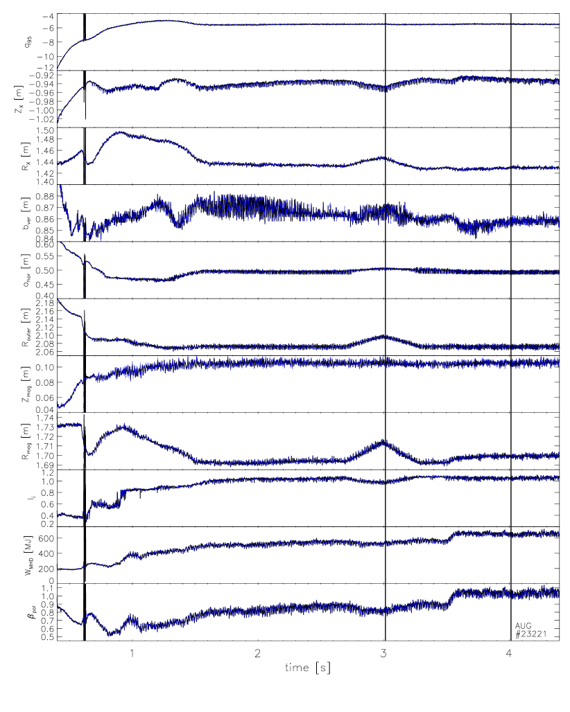
Fig. 3: Time evolution of selected parameters for AUG shot #23221 as computed with the new real-time code during an extended time window between $t=0.4~{}\mathrm{s}$ and $t=4.4~{}\mathrm{s}$. The time interval $[3.014~{}\mathrm{s},4.014~{}\mathrm{s}]$ which is chosen for performance analysis is indicated by vertical lines. The individual plots show the coordinates $(R_{\mathrm{mag}},Z_{\mathrm{mag}})$ and $(R_{\mathrm{X}},Z_{\mathrm{X}})$ of the magnetic axis, and of the x-point, respectively, the horizontal and vertical minor plasma radius, $a_{\mathrm{hor}}$ and $b_{\mathrm{ver}}$, the plasma self-inductivity, $l_{\mathrm{i}}$, the poloidal beta parameter, $\beta_{\mathrm{pol}}$, the total energy content of the plasma, $W_{\mathrm{MHD}}$, and the safety factor $q_{95}$ (see Sect. II.B for the definition of the quantities). The solid, black lines correspond to a ”real-time” application which is restricted to 4 equilibrium iterations. For comparison, values derived from converged equilibrium solutions (convergence criterion ${\lVert\psi^{i}-\psi^{i-1}\lVert}_{\infty}<10^{-4}$) are shown as dashed, blue lines. A standard spatial resolution of $(32,64)$ grid points and 7 basis functions were employed.

III APPLICATION PERFORMANCE

III.A Demonstration of Real-Time Capability

Fig. 4: Evolution of the relative deviation (denoted by square brackets) of the quantities which were computed after 4 equilibrium iterations, from the values computed with converged equilibrium solutions (convergence criterion ${\lVert\psi^{i}-\psi^{i-1}\lVert}_{\infty}<10^{-4}$) during the time interval chosen for performance analysis (as indicated by vertical lines in Fig. 3). A standard spatial resolution of $(32,64)$ grid points and 7 basis functions were employed.

In order to demonstrate the real-time capability of the new code a post-processing run is performed using data from a typical AUG discharge. We chose AUG shot number #23221, and focus on a time window between $t_{1}=3.014~{}\mathrm{s}$ and $t_{1000}=4.013~{}\mathrm{s}$ with 1000 time points, corresponding to a time resolution of exactly 1 ms. As shall be shown below this simulation of 1000 time points can be performed on standard server hardware within less than a second of computing time.

resolution	$T_{\mathrm{tot}}$	$T_{\mathrm{eq}}$	$T_{\mathrm{ctl}}$	cores	MPI	threads
$(N_{r},N_{z},N\!\!+\!\!1)$	[ms]	[ms]	[ms]	(nodes)	tasks	per task
$(32,64,6)$	0.85	0.62	0.18	24 (1)	6	4
$(32,64,8)$	1.08	0.87	0.17	24 (1)	4	6
$(32,64,8)$	0.88	0.67	0.17	48 (2)	8	6
$(32,64,12)$	0.97	0.74	0.19	72 (3)	12	6
$(32,64,16)$	1.55	1.32	0.18	24 (1)	4	6
$(32,64,16)$	1.26	1.02	0.18	48 (2)	8	6
$(32,64,16)$	0.99	0.73	0.21	96 (4)	16	6
$(64,128,6)$	2.07	1.55	0.39	48 (2)	6	8
$(64,128,8)$	1.88	1.28	0.48	48 (2)	8	6
$(64,128,12)$	2.02	1.39	0.49	72 (3)	12	6
$(64,128,16)$	2.04	1.40	0.51	96 (4)	16	6

TABLE I: Overview of the total runtime $T_{\mathrm{tot}}$ per time point ($2^{\mathrm{nd}}$ column) for different combinations of the numerical resolution ($1^{\mathrm{st}}$ column) and compute resources. The latter are given in terms of the total number of cores (nodes) ($5^{\mathrm{th}}$ column), of MPI tasks ($6^{\mathrm{th}}$ column) and of OpenMP threads per MPI task ($7^{\mathrm{th}}$ column). $T_{\mathrm{tot}}$ is the sum of the runtime $T_{\mathrm{eq}}$ ($3^{\mathrm{rd}}$ column) for computing the equilibrium distribution $\psi$ with 4 iteration steps (cf. Sect. II.A), and $T_{\mathrm{ctl}}$ ($4^{\mathrm{th}}$ column) for deriving plasma-control parameters (cf. Sect. II.B). The benchmarks were performed on Xeon E5-2680v3 ”Haswell” CPUs (2.5 GHz, 24 cores per node) and used data from AUG shot #23221.

The GPEC code computes a fixed number of four equilibrium iteration steps for every time point and uses the equilibrium solution $\psi(t_{n})$ at time point $t_{n}$ as the initial value for the next time point $t_{n+1}$. A standard spatial resolution of $(N_{r},N_{z})=(32,64)$ grid points is employed, and $N=7$ basis functions are used. The response matrix $\boldsymbol{B}$ contains signals from 61 magnetic probes and 18 flux loops and in addition takes into account 10 external coils. Figure 3 provides an overview of the time evolution of a number of characteristic parameters, such as selected plasma-shape parameters, energy content and safety factor $q_{95}$ (black, solid lines). For reference, the figure shows an extended time window between $t=0.4~{}\mathrm{s}$ and $t=4.4~{}\mathrm{s}$, which includes the dynamic start-up phase of the discharge with significant variations in the plasma parameters, and also shows results from a run which converges the solution $\psi$ until the maximum changes on the grid, ${\lVert\psi^{i}-\psi^{i-1}\lVert}_{\infty}$, are below $10^{-4}$ (blue, dashed lines). Compared with the converged reference run one notices good overall agreement of the ”real-time” simulation with a fixed number of 4 equilibrium iterations throughout the extended time interval, even during the initial start-up phase which lasts until approx. 1.5 s. It is hence justified to confine the analysis on the — arbitrarily chosen — time interval, $[3.014~{}\mathrm{s},4.013~{}\mathrm{s}]$ in the ”plateau” phase of the discharge. Focusing on this time window, Figure 4 shows that the relative errors for most quantities are at smaller than one percent. The comparably large variations of $Z_{\rm mag}$ are due to its small absolute value. The absolute scatter of $Z_{\rm mag}$ is in the order of mm. Note that the cycle time of $\Delta t=1$ ms is much shorter than the timescale of the changes of plasma conditions (cf. the increase of $W_{\mathrm{MHD}}$, $\beta_{\mathrm{pol}}$ at $t\approx 3.5$ s). Thus the equilibrium solution, even if not fully converged, can easily follow such secular trends, which is reflected by the fact that there is no visible change in the magnitudes of the relative error at $t\approx 3.5$ s.

The employed spatial resolution of $(N_{r},N_{z})=(32,64)$ grid points is a common choice for real-time analysis in medium-sized tokamaks ^{9, 7, 14, 4, 15}. For the chosen AUG discharge a comparison with a run using a twofold finer spatial grid spacing, $(N_{r},N_{z})=(64,128)$, shows good agreement for the majority of quantities, with $q_{95}$ and $R_{\mathrm{outer}}$ exhibiting the largest sensitivity to the resolution.

We conclude that by performing four iterations per time point and using $(N_{r},N_{z})=(32,64)$ spatial grid points, sufficiently accurate equilibrium solutions for deriving real-time control parameters are obtained, at least in the sense of a proof-of-principle using the chosen example data from AUG shot #23221. A systematic analysis of the accuracy and a comprehensive validation of the code under various tokamak operational scenarios is beyond the scope of this paper.

III.B Computational Performance

Overview

The computational performance of GPEC is assessed on a standard compute cluster with x86_64 CPUs and InfiniBand (FDR 14) interconnect. The individual compute nodes are equipped with two Intel Xeon E5-2680v3 ”Haswell” CPUs (2.5 GHz, 2x12 cores). We use a standard Intel software stack (FORTRAN compiler v14.0, MPI v5.0) on top of the Linux operating system (SLES11 SP3). For the required linear algebra functionality the OpenBLAS ²⁸ library (version 0.2.13) is employed using the de-facto-standard interfaces from BLAS ^{29, 30} and LAPACK ^{31, 30}, and the FFTW ³² library (version 3.3.4) is used for the discrete sine transforms in the Poisson solver. Both libraries are open-source software released under the BSD or the GPL license, respectively. If desired, open-source alternatives to the Intel compilers (e.g. GCC ³³) and MPI libraries (e.g. OpenMPI ³⁴, MVAPICH ³⁵) could be readily utilized, albeit possibly with a certain performance impact.

Table I shows an overview of the total runtime per time point and of the individual contributions from computing the equilibrium solution and from deriving the set of plasma-control parameters. We chose combinations of different numerical resolutions (in terms of the spatial grid resolution $N_{r}\times N_{z}$ and number of basis functions $N$) and computing resources (in terms of the number of CPU cores).

With two compute nodes (each with 24 CPU cores) and using a resolution of $(N_{r},N_{z},N\!+\!1)=(32,64,8)$ a runtime well below 1 ms and hence real-time capability is reached. When doubling the number of basis functions ($N\!+\!1\!=\!16$) real-time calculation is still possible on four compute nodes, indicating overall good weak scalability of the code.

Roughly three quarters of the runtime is required for computing the equilibrium solution and the rest goes into evaluating the set of plasma control parameters. Hence, with a reduction of the number of equilibrium iterations to only one or two ^{13, 14, 4, 15} runtimes of 0.5 ms are reached on just a single compute server.

With a higher spatial resolution of $(N_{r},N_{z})=(64,128)$ a cycle time of 2 ms is possible with 4 iterations, although from the linear algorithmic complexity of the algorithm ¹⁸, and the amount of data which is communicated between the processes one would expect the runtime to increase by a factor of four compared to $(N_{r},N_{z})=(32,64)$. The reason is a higher parallel efficiency of the Poisson solver which is limited by OpenMP overhead at lower resolutions ¹⁸ as well as lower communication overhead due to larger message sizes in the expensive MPI_Allreduce operation which collects the distributed fields $\psi_{k}(r,z)$ and computes the sum $\psi=\sum_{k=1}^{N}c_{k}\psi_{k}$ (see the rows labelled ”Poisson solver” and ”$\psi$ sum” in Table II).

resolution $(N_{r},N_{z},N\!\!+\!\!1)$	$(32,64,8)$		$(32,64,16)$		$(64,128,8)$		$(64,128,16)$
cores (MPI tasks $\cdot$ threads/task)	$48(8\cdot 6)$		$96(16\cdot 6)$		$48(8\cdot 6)$		$96(16\cdot 6)$
	$T$ [ms]	%	$T$ [ms]	%	$T$ [ms]	%	$T$ [ms]	%
RHS update	0.022	13.2	0.021	11.7	0.050	15.7	0.053	15.0
Poisson solver	0.036	21.6	0.036	19.5	0.085	26.6	0.086	24.5
RM evaluation	0.024	14.5	0.024	13.3	0.025	7.8	0.025	7.1
RM gather∗	0.015	8.9	0.021	11.4	0.019	5.9	0.029	8.1
lin. regression	0.013	7.9	0.017	9.5	0.014	4.4	0.018	5.2
$\psi$ sum∗∗	0.048	28.9	0.056	30.5	0.110	36.2	0.128	36.2
other	0.008	5.0	0.008	4.2	0.011	3.4	0.014	3.9
total	0.167	100.0	0.182	100.0	0.319	100.0	0.353	100.0

TABLE II: Runtime breakdown of a single Picard equilibrium-iteration step (average over 4 iteration steps times 1000 time points) for different combinations (subset of Table I) of numerical resolution and computational resources. The individual algorithmic steps from top to bottom correspond to the sequence in Sect. II.A. Routines labelled with asterisks are dominated by MPI communication (^∗MPI_Allgather, ^∗∗MPI_Allreduce).

Equilibrium reconstruction

Table II further shows that the runtime for the equilibrium iterations is dominated by computing the distributed sum, $\psi=\sum_{k=1}^{N}c_{k}\psi_{k}$, which is also an implicit synchronization point for all processes, and by the Poisson solver. Due to the use of high-order interpolation schemes (cf. Sect.II.A) a significant fraction of about 25% is spent on the evaluation of the right-hand sides of Eqs. (5,6) (”RHS update”) and of the response matrix $\boldsymbol{B}$ (”RM evaluation”).

In general, the chosen products of number of MPI tasks times OpenMP threads per task turned out as the most efficient ones for this hardware platform with 24 cores per node: using more than 6 threads (or 8 threads in the case of $(N_{r},N_{z})=(64,128)$) results only in a modest speedup of the Poisson solver ¹⁸ but doubles the required number of cores and network resources. Keeping those constant and reducing the number of MPI tasks instead by a factor of two would require each MPI task to handle two basis functions. Although the collective MPI communications would be somewhat faster in this case the resultant doubling of the effective runtime for the Poisson solver cannot be compensated for.

Plasma-control parameters

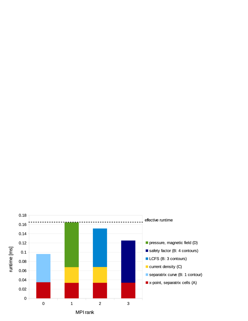
Fig. 5: Runtime of the major groups (A-D) of computations for the plasma-control parameters (cf. Sect. II.B) and their assignment to four MPI tasks which execute in parallel. Within each task the individual parts of the algorithm (indicated by different colours) execute in the order from bottom to top. Accordingly, the dashed horizontal line marks the effective runtime in the application. The data corresponds to AUG shot #23221 computed with a resolution of $(N_{r},N_{z},N\!+\!1)=(32,64,8)$ using in total 8 MPI tasks, each with 6 OpenMP threads (cf. Table I).

For the example of $(N_{r},N_{z},N+1)=(32,64,8)$ computed with 48 CPU cores, Figure 5 shows how the runtime of $T_{\mathrm{ctl}}=0.17$ ms (cf. Table I) is composed and illustrates the benefits of exploiting task parallelism. Due to the final MPI_Allreduce operation in the equilibrium construction algorithm, which comes at little extra effective runtime cost as compared to a single MPI_Reduce, all MPI tasks hold a copy of the equilibrium flux distribution $\psi(r,z)$. Hence, independent parts of the time-consuming computations for the plasma-control parameters like, e.g. evaluating the pressure distribution or determining the contours for the safety factor $q$, can be handled in parallel by different MPI tasks and only scalar quantities need to be communicated (within a few microseconds) between the MPI tasks at the end. If necessary, the remaining load-imbalance indicated by Figure 5, namely task 0 and task 3 becoming idle after about 0.1 ms, and tasks $4,\dotsc,7$ not computing anything at all at this stage, could be exploited for computing additional quantities and/or for further reducing the effective runtime. Without task-parallelization, on the contrary, the runtimes would add up to more than 0.4 ms despite the thorough OpenMP parallelization (e.g. across different contour levels) within the task.

IV CONCLUSIONS

With the motivation of achieving sub-millisecond runtimes a new, parallel equilibrium-reconstruction code, GPEC, was presented which is suitable for real-time applications in medium-sized tokamaks like ASDEX Upgrade (AUG). GPEC implements the classical concept of iteratively solving the Grad-Shafranov equation and feeding in diagnostic signals from the experiment ^{7, 8}. Specifically, GPEC is implemented as a variant of the IDE code ¹⁹, which is a descendant of CLISTE ⁸. Compared with these well-established and validated offline-analysis codes no algorithmic simplifications are necessary for achieving the desired cycle times of less than a millisecond, besides limiting the number of equilibrium iterations to four. In addition to real-time applications the new code enables fast and highly accurate offline analyses soon after the tokamak discharge: Here, tolerable runtimes are in the range of 0.1–1 s per cycle which allows computing fully converged equilibria employing highly resolved spatial and basis functions grids.

The parallelization of the new code builds on a fast shared-memory-parallel Grad-Shafranov solver ¹⁸ together with the MPI-distributed solution of the individual Poisson-type problems and a thorough parallelization of the post-processing algorithms for computing the relevant plasma-control parameters from the equilibrium flux distribution.

Using data from a typical AUG discharge the real-time capability of the new code was demonstrated by the offline computation of a sequence of 1000 time points within less than a second of runtime. The relative accuracy was ascertained by comparing the relevant plasma parameters with a converged run. By allowing four iterations for computing the equilibrium solution the majority of control parameters can be computed with an accuracy of a percent or better.

The adopted two-level, hybrid parallelization scheme allow efficient utilization available compute resources (in terms of the numbers of nodes, of CPU sockets per node and of cores per socket) for a given numerical resolution (in terms of the spatial grid and number of basis functions). Moreover, foreseeable advances in computer technology, in particular the increasing number of CPU cores per compute node, are expected to push the limits of real-time applications with GPEC towards even higher numerical accuracies (in terms of affordable resolution and number of equilibrium iterations). We note that the benchmarks figures reported in this work can be considered rather conservative as the computations were performed on a standard compute cluster which comprises hundreds of nodes. For energy-budget reasons such clusters are typically configured not with CPUs of the highest clock-frequency. In our case, for example, CPUs with 2.5 GHz and only 24 cores per node were available. For deployment in the control system of a tokamak experiment such as AUG, by contrast, we envision dedicated server hardware with higher clock frequencies and at least four CPU sockets, both of which is expected to further boost the computational performance of the real-time application. Thus it should be rather straightforward to save enough time for the communication of the code with the control system, which, depending of the specifics of the system, requires another few hundred microseconds per cycle.

Finally, it is worth mentioning that GPEC is based entirely on open-source software components, relies on established industry (FORTRAN, MPI, OpenMP) or de-facto software standards (BLAS, LAPACK, FFTW), runs on standard server hardware and software environments and hence can be released to the community and utilized without legal or commercial restrictions.

References

- 1 C. GORMEZANO, A. SIPS, T. LUCE, S. IDE, A. BECOULET, X. LITAUDON, A. ISAYAMA, J. HOBIRK, M. WADE, T. OIKAWA, R. PRATER, A. ZVONKOV, B. LLOYD, T. SUZUKI, E. BARBATO, P. BONOLI, C. PHILLIPS, V. VDOVIN, E. JOFFRIN, T. CASPER, J. FERRON, D. MAZON, D. MOREAU, R. BUNDY, C. KESSEL, A. FUKUYAMA, N. HAYASHI, F. IMBEAUX, M. MURAKAMI, A. POLEVOI, & H. S. JOHN. Chapter 6: Steady state operation. Nuclear Fusion, 47(6), S285 (2007).
- 2 Y. GRIBOV, D. HUMPHREYS, K. KAJIWARA, E. LAZARUS, J. LISTER, T. OZEKI, A. PORTONE, M. SHIMADA, A. SIPS, & J. WESLEY. Chapter 8: Plasma operation and control. Nuclear Fusion, 47(6), S385 (2007).
- 3 M. MARASCHEK, G. GANTENBEIN, T. P. GOODMAN, S. GÜNTER, D. F. HOWELL, F. LEUTERER, A. MÜCK, O. SAUTER, & H. ZOHM. Active control of MHD instabilities by ECCD in ASDEX upgrade. Nuclear Fusion, 45, 1369 (2005).
- 4 L. GIANNONE, M. REICH, M. MARASCHEK, C. RAPSON, W. TREUTTERER, L. BARRERA, E. POLI, A. BOCK, G. CONWAY, F. FISCHER, J. FUCHS, K. LACKNER, P. MCCARTHY, A. MLYNEK, R. PREUSS, K.-H. SCHUHBECK, J. STOBER, M. RAMPP, R. MCDERMOTT, Q. RUAN, L. WENZEL, & ASDEX UPGRADE TEAM. A data acquisition system for real-time magnetic equilibrium reconstruction on ASDEX Upgrade and its application to NTM stabilization experiments. Fusion Engineering and Design, 88, 3299 (2013).
- 5 V. D. SHAFRANOV. About MHD equilibrium configurations. Zh. Eksp. Teor. Fiz., 33, 710 (1957).
- 6 R. LÜST & A. SCHLÜTER. Axisymmetrische magnetohydrodynamische Gleichgewichtskonfigurationen. Z. Naturforsch., 129, 850 (1957).
- 7 L. L. LAO, J. R. FERRON, R. J. GROEBNER, W. HOWL, H. ST. JOHN, E. J. STRAIT, & T. S. TAYLOR. Equilibrium analysis of current profiles in tokamaks. Nuclear Fusion, 30, 1035 (1990).
- 8 P. J. MCCARTHY, P. MARTIN, & W. SCHNEIDER. The CLISTE interpretive equilibrium code. Tech. Rep. IPP 5/85, Max-Planck-Institut für Plasmaphysik (1999).
- 9 L. LAO, H. S. JOHN, R. STAMBAUGH, A. KELLMAN, & W. PFEIFFER. Reconstruction of current profile parameters and plasma shapes in tokamaks. Nuclear Fusion, 25(11), 1611 (1985).
- 10 J. BLUM, C. BOULBE, & B. FAUGERAS. Reconstruction of the equilibrium of the plasma in a tokamak and identification of the current density profile in real time. Journal of Computational Physics, 231(3), 960 (2012).
- 11 B. BRAAMS, W. JILGE, & K. LACKNER. Fast determination of plasma parameters through function parametrization. Nuclear Fusion, 26(6), 699 (1986).
- 12 L. GIANNONE, M. CERNA, R. COLE, M. FITZEK, A. KALLENBACH, K. LüDDECKE, P. MCCARTHY, A. SCARABOSIO, W. SCHNEIDER, A. SIPS, W. TREUTTERER, A. VRANCIC, L. WENZEL, H. YI, K. BEHLER, T. EICH, H. EIXENBERGER, J. FUCHS, G. HAAS, G. LEXA, M. MARQUARDT, A. MLYNEK, G. NEU, G. RAUPP, M. REICH, J. SACHTLEBEN, K. SCHUHBECK, T. ZEHETBAUER, S. CONCEZZI, T. DEBELLE, B. MARKER, M. MUNROE, N. PETERSEN, & D. SCHMIDT. Data acquisition and real-time signal processing of plasma diagnostics on ASDEX upgrade using labview RT. Fusion Engineering and Design, 85(3–4), 303 (2010). Proceedings of the 7th IAEA Technical Meeting on Control, Data Acquisition, and Remote Participation for Fusion Research.
- 13 X. N. YUE, B. J. XIAO, Z. P. LUO, & Y. GUO. Fast equilibrium reconstruction for tokamak discharge control based on GPU. Plasma Physics and Controlled Fusion, 55(8), 085016 (2013).
- 14 A. BARP, M. CERNA, S. CONCEZZI, L. GIANNONE, G. MORROW, Q. RUAN, A. VEERAMANI, & L. WENZEL. A real-time Grad-Shafranov PDE solver and MIMO controller. Fusion Engineering and Design, 87(12), 2112 (2012). Proceedings of the 8th IAEA Technical Meeting on Control, Data Acquisition, and Remote Participation for Fusion Research.
- 15 J.-M. MORET, B. DUVAL, H. LE, S. CODA, F. FELICI, & H. REIMERDES. Tokamak equilibrium reconstruction code LIUQE and its real time implementation. Fusion Engineering and Design, 91, 1 (2015).
- 16 J. FERRON, M. WALKER, L. LAO, H. S. JOHN, D. HUMPHREYS, & J. LEUER. Real time equilibrium reconstruction for tokamak discharge control. Nuclear Fusion, 38, 1055 (1998).
- 17 I. YONEKAWA, A. V. FERNANDEZ, J.-M. FOURNERON, J.-Y. JOURNEAUX, W.-D. KLOTZ, A. WALLANDER, & CODAC TEAM. ITER instrumentation and control system towards long pulse operation. Plasma Fusion Research, 7, 2505047 (2012).
- 18 M. RAMPP, R. PREUSS, R. FISCHER, K. HALLATSCHEK, & L. GIANNONE. A parallel Grad-Shafranov solver for real-time control of tokamak plasmas. Fusion Science and Technology, 62(3), 409 (2012).
- 19 R. FISCHER, J. HOBIRK, L. B. ORTE, A. BOCK, A. BURCKHART, I. CLASSEN, M. DUNNE, J. FUCHS, L. GIANNONE, K. LACKNER, P. MCCARTHY, R. PREUSS, M. RAMPP, S. RATHGEBER, M. REICH, B. SIEGLIN, W. SUTTROP, E. WOLFRUM, & ASDEX UPGRADE TEAM. Magnetic equilibrium reconstruction using geometric information from temperature measurements at asdex upgrade. In V. NAULIN, C. ANGIONI, M. BORGHESI, S. RATYNSKAIA, S. POEDTS, & T. DONNé (eds.), 40th EPS Conference on Plasma Physics, vol. 37D of Europhysics conference abstracts, page P2.139. European Physical Society, Geneva (2013).
- 20 P. J. MCCARTHY & ASDEX UPGRADE TEAM. Identification of edge-localized moments of the current density profile in a tokamak equilibrium from external magnetic measurements. Plasma Physics and Controlled Fusion, 54(1), 015010 (2012).
- 21 A. E. HOERL & R. W. KENNARD. Ridge regression: Biased estimation for nonorthogonal problems. Technometrics, 12(1), 55 (1970).
- 22 W. H. PRESS, S. A. TEUKOLSKY, W. T. VETTERLING, & B. P. FLANNERY. Numerical Recipes: The Art of Scientific Computing. Cambridge University Press, 3rd edn. (2007).
- 23 K. V. HAGENOW & K. LACKNER. Computation of axisymmetric MHD equilibria. In Proc. 7th Conf. on the Numerical Simulation of Plasmas, page 140. New York, US (1975).
- 24 K. LACKNER. Computation of ideal MHD equilibria. Comp. Phys. Comm., 12, 33 (1976).
- 25 R. PREUSS, R. FISCHER, M. RAMPP, K. HALLATSCHEK, U. VON TOUSSAINT, L. GIANNONE, & P. MCCARTHY. Parallel equilibrium algorithm for real-time control of tokamak plasmas. Tech. Rep. IPP R/47, Max-Planck-Institut für Plasmaphysik (2012).
- 26 http://www.mpi-forum.org/.
- 27 W. M. STACEY. Fusion Plasma Physics. Wiley, 2 edn. (2012).
- 28 http://www.openblas.net.
- 29 BLAST FORUM. Basic linear algebra subprograms technical forum standard. International Journal of High Performance Applications and Supercomputing, 16(1) (2002).
- 30 http://www.netlib.org.
- 31 E. ANDERSON, Z. BAI, C. BISCHOF, S. BLACKFORD, J. DEMMEL, J. DONGARRA, J. DU CROZ, A. GREENBAUM, S. HAMMARLING, A. MCKENNEY, & D. SORENSEN. LAPACK Users’ Guide. Society for Industrial and Applied Mathematics, Philadelphia, PA, third edn. (1999). ISBN 0-89871-447-8 (paperback).
- 32 M. FRIGO & S. G. JOHNSON. The design and implementation of FFTW3. Proceedings of the IEEE, 93(2), 216 (2005). Special issue on “Program Generation, Optimization, and Platform Adaptation”.
- 33 https://gcc.gnu.org/.
- 34 http://www.open-mpi.de/.
- 35 http://mvapich.cse.ohio-state.edu/.