Submitted to Proceedings of the National Academy of Sciences of the United States of America \urlwww.pnas.org/cgi/doi/10.1073/pnas.XXXXXXXXXX \issuedateIssue Date \issuenumberIssue Number
Submitted to Proceedings of the National Academy of Sciences of the United States of America
Growing timescales and lengthscales characterizing vibrations of amorphous solids
Abstract
Low-temperature properties of crystalline solids can be understood using harmonic perturbations around a perfect lattice, as in Debye’s theory. Low-temperature properties of amorphous solids, however, strongly depart from such descriptions, displaying enhanced transport, activated slow dynamics across energy barriers, excess vibrational modes with respect to Debye’s theory (i.e., a Boson Peak), and complex irreversible responses to small mechanical deformations. These experimental observations indirectly suggest that the dynamics of amorphous solids becomes anomalous at low temperatures. Here, we present direct numerical evidence that vibrations change nature at a well-defined location deep inside the glass phase of a simple glass former. We provide a real-space description of this transition and of the rapidly growing time and length scales that accompany it. Our results provide the seed for a universal understanding of low-temperature glass anomalies within the theoretical framework of the recently discovered Gardner phase transition.
keywords:
Low-temperature amorphous solids — marginal glasses — Gardner transition
Significance
Amorphous solids constitute most of
solid matter but remain poorly understood.
The recent solution of the mean-field hard sphere glass former provides,
however, deep insights into their material properties. In
particular, this solution predicts a Gardner transition below which
the energy landscape of glasses becomes fractal and the solid is
marginally stable. Here we provide the first direct evidence for the
relevance of a Gardner transition in physical systems. This result thus
opens the way towards a unified understanding of the
low-temperature anomalies of amorphous solids.
Introduction -
Understanding the nature of the glass transition, which describes the gradual transformation of a viscous liquid into an amorphous solid, remains an open challenge in condensed matter physics [1, 2]. As a result, the glass phase itself is not well understood either. The main challenge is to connect the localised, or ‘caged’, dynamics that characterizes the glass transition to the low-temperature anomalies that distinguish amorphous solids from their crystalline counterparts [3, 4, 5, 6, 7]. Recent theoretical advances, building on the random first-order transition approach [8], have led to an exact mathematical description of both the glass transition and the amorphous phases of hard spheres in the mean-field limit of infinite-dimensional space [9]. A surprising outcome has been the discovery of a novel phase transition inside the amorphous phase, separating the localised states produced at the glass transition from their inherent structures. This Gardner transition [10], which marks the emergence of a fractal hierarchy of marginally stable glass states, can be viewed as a glass transition deep within a glass, at which vibrational motion dramatically slows down and becomes spatially correlated [11]. Although these theoretical findings promise to explain and unify the emergence of low-temperature anomalies in amorphous solids, the gap remains wide between mean-field calculations [9, 11] and experimental work. Here, we provide direct numerical evidence that vibrational motion in a simple three-dimensional glass-former becomes anomalous at a well-defined location inside the glass phase. In particular, we report the rapid growth of a relaxation time related to cooperative vibrations, a non-trivial change in the probability distribution function of a global order parameter, and the rapid growth of a correlation length. We also relate these findings to observed anomalies in low-temperature laboratory glasses. These results provide key support for a universal understanding of the anomalies of glassy materials, as resulting from the diverging length and time scales associated with the criticality of the Gardner transition.
Preparation of glass states –
Experimentally, glasses are obtained by a slow thermal or compression annealing, the rate of which determines the location of the glass transition [1, 2]. We find that a detailed numerical analysis of the Gardner transition requires the preparation of extremely well-relaxed glasses (corresponding to structural relaxation timescales challenging to simulate) in order to study vibrational motion inside the glass without interference from particle diffusion. We thus combine a very simple glass-forming model – a polydisperse mixture of hard spheres – to an efficient Monte-Carlo scheme to obtain equilibrium configurations at unprecedentedly high densities, i.e., deep in the supercooled regime. The optimized swap Monte-Carlo algorithm [12], which combines standard local Monte-Carlo moves with attempts at exchanging pairs of particle diameters, indeed enhances thermalization by several orders of magnitude. Configurations contain either or (results in Figs. 1-3 are for , and for in Fig. 4) hard spheres with equal unit mass and diameters independently drawn from a probability distribution , for . We similarly study a two-dimensional bidisperse model glass former and report the main results in the Appendix.
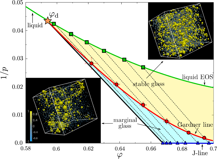
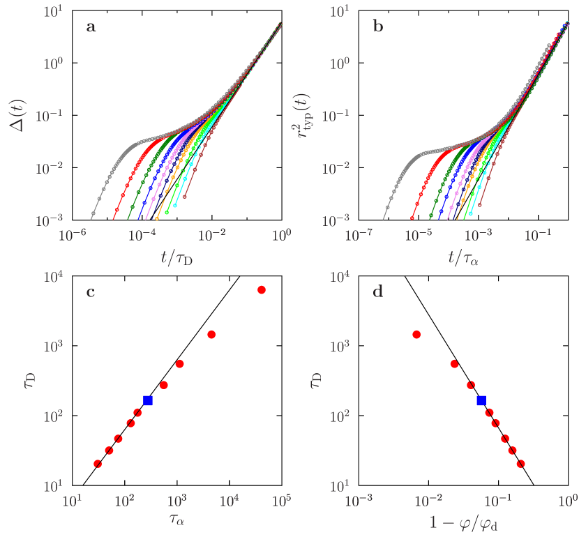
We mimic slow annealing in two steps (Fig. 1). First, we produce equilibrated liquid configurations at various densities using our efficient simulation scheme, concurrently obtaining the liquid equation of state (EOS). The liquid EOS for the reduced pressure , where is the number density, is the inverse temperature, and is the system pressure, is described by
| (1) |
with from Ref. [13]:
| (2) |
where is the -th moment of , and are fitted quantities. The structure of the equilibrium configurations generated by the swap algorithm has been carefully analyzed. Unlike for other glass formers [14, 15], no signs of orientational or crystalline order were observed [16, 17]. Following the strategy of Ref. [18], we also obtain the dynamical crossover (see the Appendix). We have not analyzed the compression of equilibrium configurations with , as done in earlier studies [19, 20], because structural relaxation is not well decoupled from vibrational dynamics, although the obtained jammed states should have equivalent properties.
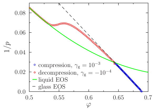
Second, we use these liquid configurations as starting points for standard molecular dynamics simulations during which the system is compressed out of equilibrium up to various target [21]. Annealing is achieved by growing spheres following the Lubachevsky-Stillinger (LS) algorithm [21] at a constant growth rate (see the Appendix for a discussion on the -dependence). The average particle diameter, , serves as unit length, and the simulation time is expressed in units of , with unit inverse temperature and unit mass . In order to obtain thermal and disorder averaging, this procedure is repeated over samples ( for and for ), each with different initial equilibrium configurations at , and over independent thermal (quench) histories for each sample. Quantities reported here are averaged over quench histories, unless otherwise specified. The non-equilibrium glass EOSs associated with this compression (dashed lines) terminate (at infinite pressure) at inherent structures that correspond, for hard spheres, to jammed configurations (blue triangles). In order to capture the glass EOSs, we use a free volume scaling around the corresponding jamming point ,
| (3) |
where the constant weakly depends on .
Our numerical protocol is analogous to varying the cooling rate – and thus the glass transition temperature – of thermal glasses, and then further annealing the resulting amorphous solid. Each value of indeed selects a different glass, ranging from the onset of sluggish liquid dynamics around the mode-coupling theory dynamical crossover [2, 1], , to the very dense liquid regime where diffusion and vibrations (-relaxation processes) are fully separated [2]. For sufficiently large , we thus obtain unimpeded access to the only remaining glass dynamics, i.e., -relaxation processes [4].
Growing timescales –
A central observable to characterize glass dynamics is the mean-squared displacement (MSD) of particles from position ,
| (4) |
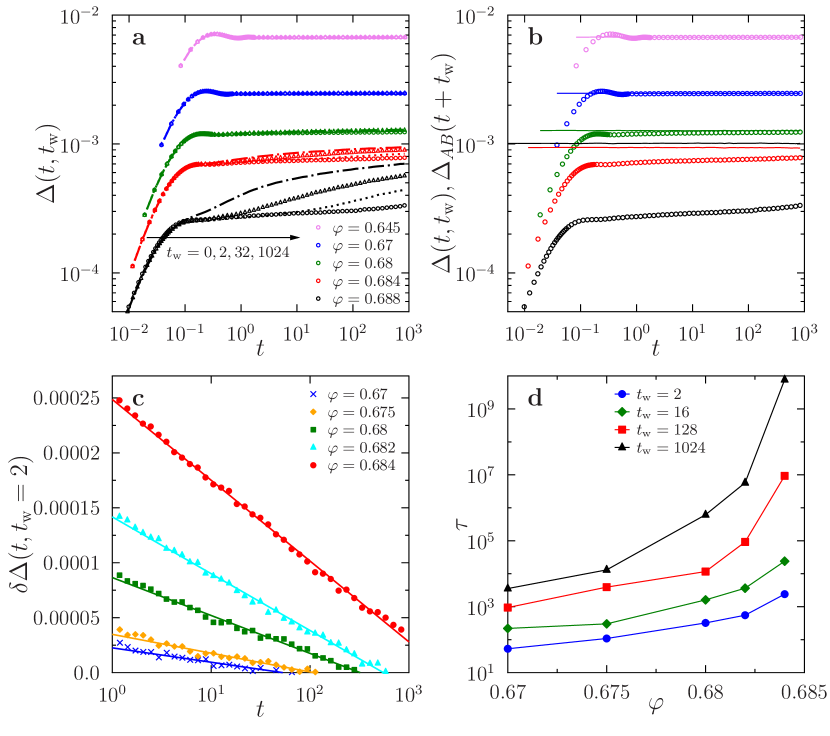
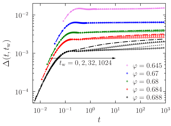
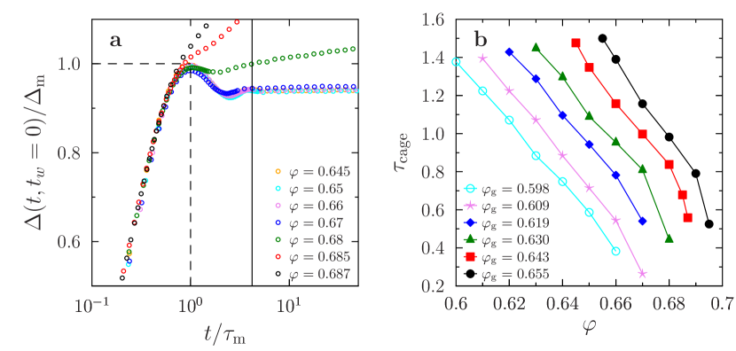
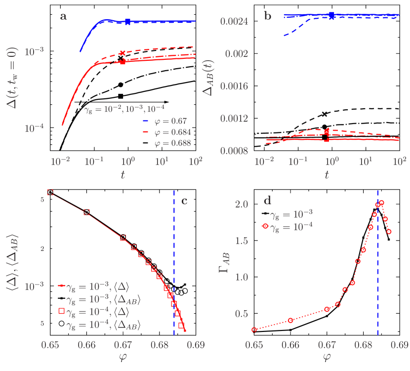
averaged over both thermal fluctuations and disorder, where time starts after waiting time when compression has reached the target . The MSD plateau height at long times quantifies the average cage size (see the Appendix). Because some of the smaller particles manage to leave their cages, the sum in Eq. (4) is here restricted to the larger half of the particle size distribution (see the Appendix). When is not too large, , the plateau emerges quickly, as suggested by the traditional view of caging in glasses (Fig. 2a). When the glass is compressed beyond a certain , however, displays both a strong dependence on the waiting time , i.e., aging, and a slow dynamics, as captured by the emergence of two plateaux.
These effects suggest a complex vibrational dynamics. Aging, in particular, provides a striking signature of a growing timescale associated with vibrations, revealing the existence of a “glass transition” deep within the glass phase.
To determine the timescale associated with this slowdown, we estimate the distance between independent pairs of configurations by first compressing two independent copies, and , from the same initial state at to the target , and then measuring their relative distance
| (5) |
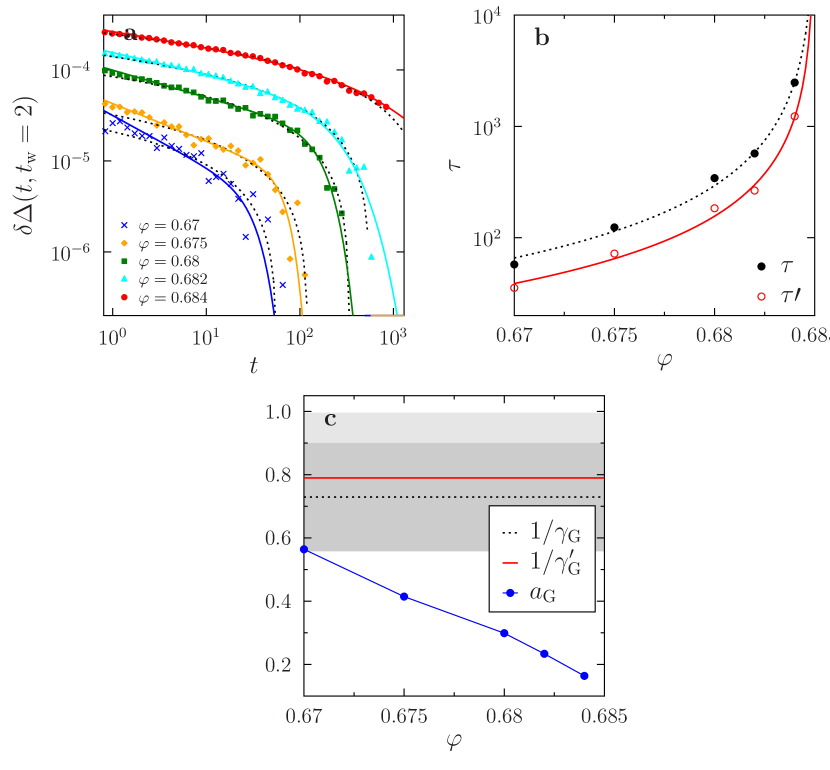
so that , as shown in Fig. 2b. The two copies share the same positions of particles at , but are assigned different initial velocities drawn from the Maxwell–Boltzmann distribution. The time evolution of the difference indicates that whereas the amplitude of particle motion naturally becomes smaller as increases, the corresponding dynamics becomes slower (Fig. 2c). In other words, as grows particles take longer to explore a smaller region of space. In a crystal, by contrast, decays faster under similar circumstances. A relaxation timescale, , can be extracted from the decay of at large , whose logarithmic form, , is characteristic of the glassiness of vibrations. As , we find that dramatically increases (Fig. 2d), which provides direct evidence of a marked crossover characterizing the evolution of the glass upon compression.
Global fluctuations of the order parameter –
This sharp dynamical crossover corresponds to a loss of ergodicity inside the glass, i.e., time and ensemble averages yield different results. To better characterize this crossover, we define a timescale for the onset of caging (, see the Appendix), and the corresponding order parameters and .
The evolution of the probability distribution functions, and , as well as their first moments, and , are presented in Figs. 3a,b for a range of densities across . For , dynamics is fast, and coincide, and and are narrow and Gaussian-like. For , however, the MSD does not converge to its long-time limit, , which indicates that configuration space explored by vibrational motion is now broken into mutually inaccessible regions. Interestingly, the slight increase of with in this regime (Fig. 3b) suggests that states are then pushed further apart in phase space, which is consistent with theoretical predictions [11]. When compressing a system across , its dynamics explores only a restricted part of phase space. As a result, displays pronounced, non-Gaussian fluctuations (Fig. 3a). Repeated compressions from a same initial state at may end up in distinct states, which explains why is typically much larger and more broadly fluctuating than (Fig. 3a). These results are essentially consistent with theoretical predictions [9, 11], which suggest that for , should separate into two peaks connected by a wide continuous band with the left-hand peak continuing the single peak of . The very broad distribution of further suggests that spatial correlations develop as , yielding strongly correlated states at larger densities.
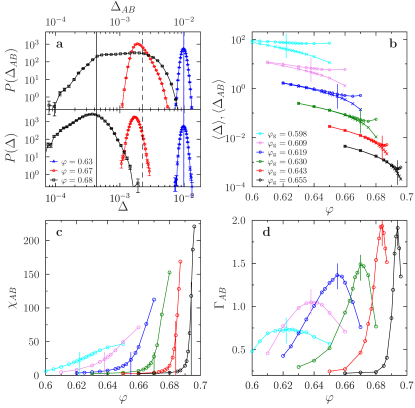
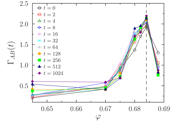
To quantify these fluctuations we measure the variance and skewness (see the Appendix and Ref. [11] ) of (Figs. 3c,d). The global susceptibility is very small for and grows rapidly as is approached, increasing by about two decades for the largest considered (Fig. 3c). While quantifies the increasing width of the distributions, reveals a change in their shapes. For each we find that is small on both sides of with a pronounced maximum at (Fig. 3d). This reflects the roughly symmetric shape of around on both sides of and the development of an asymmetric tail for large around the crossover, a known signature of sample-to-sample fluctuations in spin glasses [22] and mean-field glass models [11]. Note that because the skewness maximum gives the clearest numerical estimate of , we use it to determine the values reported in Fig. 1.
Growing correlation length –
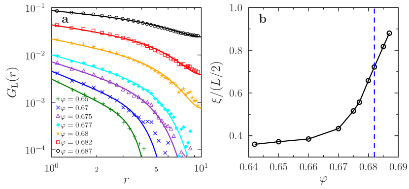
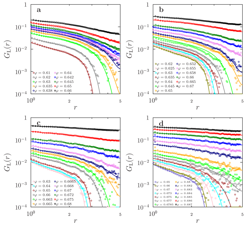
The rapid growth of in the vicinity of suggests the concomitant growth of a spatial correlation length, . Its measurement requires spatial resolution of the fluctuations of , hence for each particle we define to capture its contribution to deviations around the average . A first glimpse of these spatial fluctuations is offered by snapshots of the field (Fig. 1), which appear featureless for , but highly structured and spatially correlated for . More quantitatively, we define the spatial correlator,
| (6) |
where is the projection of the particle position along direction . Even for the larger system size considered, measuring is challenging because spatial correlations quickly become long ranged as (see Fig. 4a). Fitting the results to an empirical form that takes into account the periodic boundary conditions in a system of linear size ,
| (7) |
where and are fitting parameters, nonetheless confirms that grows rapidly with and becomes of the order of the simulation box at (Fig. 4b). Note that although probed using a dynamical observable, the spatial correlations captured by are conceptually distinct from the dynamical heterogeneity observed in supercooled liquids [23], which is transient and disappears once the diffusive regime is reached.
Experimental consequences –
The system analysed in this work is a canonical model for colloidal suspensions and granular media. Hence, experiments along the lines presented here could be performed to investigate more closely vibrational dynamics in colloidal and granular glasses, using a series of compressions to extract and . Experiments are also possible in molecular and polymeric glasses, for which the natural control parameter is temperature instead of density. Let us therefore rephrase our findings from this viewpoint. As the system is cooled, the supercooled liquid dynamics is arrested at the laboratory glass transition temperature . As the resulting glass is further cooled its phase space transforms, around a well-defined Gardner temperature , from a simple state (akin to that of a crystal) into a more complex phase composed of a large number of glassy states (see the Appendix for a discussion of the phase diagram as a function of ).
Around , vibrational dynamics becomes increasingly heterogeneous (Fig. 1), slow (Fig. 2), fluctuating from realization to realization (Fig. 3), and spatially correlated (Fig. 4). The -relaxation dynamics inside the glass thus becomes highly cooperative [24, 25] and ages [26]. The fragmentation of phase space below also gives rise to a complex response to mechanical perturbations in the form of plastic irreversible events, in which the system jumps from one configuration to another [4, 6, 27]. This expectation stems from the theoretical prediction that the complex phase at is marginally stable [9], which implies that glass states are connected by very low energy barriers, resulting in strong responses to weak perturbations [7].
A key prediction is that the aforementioned anomalies appear simultaneously around a that is strongly dependent on the scale selected by the glass preparation protocol. Annealed glasses with lower are expected to present a sharper Gardner-like crossover, at an increasingly lower temperature. Numerically, we produced a substantial variation of by using an efficient Monte-Carlo algorithm to bypass the need for a broad range of compression rates. In experiments a similar or even larger range of can be explored [28], using poorly annealed glasses from hyperquenching [29] and ultrastable glasses from vapor deposition [30, 31, 32]. We expect ultrastable glasses, in particular, to display strongly enhanced glass anomalies, consistent with recent experimental reports [33, 34, 35]. Interestingly, a Gardner-like regime may also underlie the anomalous aging recently observed in individual proteins [36].
Conclusion –
Since its prediction in the mean-field limit, the Gardner transition has been regarded as a key ingredient to understand the physical properties of amorphous solids. Understanding the role of finite dimensional fluctuations is a difficult theoretical problem [37]. Our work shows that clear signs of an apparent critical behaviour can be observed in three dimensions, at least in a finite-size system, which shows that the correlation length becomes at least comparable to the system size as approaches . Although the fate of these findings in the thermodynamic limit remains an open question, the remarkably large signature of the effect strongly suggests that the Gardner phase transition paradigm is a promising theoretical framework for a universal understanding of the anomalies of solid amorphous materials, from granular materials to glasses, foams and proteins.
Acknowledgements.
P.C. acknowledges support from the Alfred P. Sloan Foundation and NSF support No. NSF DMR-1055586. B.S. acknowledges the support by MINECO (Spain) through research contract No. FIS2012-35719-C02. This project has received funding from the European Union’s Horizon 2020 research and innovation programme under the Marie Skłodowska-Curie grant agreement No. 654971 as well as from the European Research Council under the European Union’s Seventh Framework Programme (FP7/2007-2013)/ERC grant agreement No. 306845. This work was granted access to the HPC resources of MesoPSL financed by the Region Ile de France and the project Equip@Meso (reference ANR-10-EQPX-29-01) of the programme Investissements d’Avenir supervised by the Agence Nationale pour la Recherche.All the results discussed in this Appendix have been obtained using molecular dynamics (MD) simulations, starting from the initial states produced using the swap algorithm as explained in the main text.
Appendix A Dynamical crossover density
We follow the strategy developed in Ref. [18] to determine the location of the dynamical (mode-coupling theory – MCT) crossover . (i) We obtain the diffusion time , where is the long-time diffusivity and the average particle diameter, , is also the unity of length. At long times, the mean-squared displacement (MSD) is dominated by the diffusive behavior (Fig. 5a). Note that we here ignore the dependence of on (compared with Eq. (1) in the main text), because we are interested in equilibrium liquid states below , where no aging is observed. (ii) We determine the structural relaxation time by collapsing the mean-squared typical displacement (MSTD) in the caging regime (Fig. 5b), where the typical displacement is defined as . (iii) We find the
density threshold for the breakdown of Stokes-Einstein relation (SER), , where is the shear viscosity. Because and in this regime, the SER can be rewritten as (Fig. 5c). (iv) We fit the time in the SER regime () to the MCT scaling
(or equivalently, )
to extract (Fig. 5d).
Appendix B Decompression of equilibrium configurations above the dynamical crossover
The equilibrium liquid configurations obtained from the Monte-Carlo swap algorithm are in the deeply supercooled regime , where the structural -relaxation and thus diffusion are both strongly suppressed. As long as is sufficiently far beyond , the MSD for exhibits a well-defined plateau, and the diffusive regime is not observed in the MD simulation window (see Figs. 2a and 2b in the main text). To further reveal the separation between the - and -relaxations, we decompress the equilibrium configuration and show that the resulting equation of state (EOS) follows the free-volume glass EOS ( Eq. (3) in the main text) up to a threshold density, at which the system melts into a liquid (Fig. 6). This behavior suggests that our compression/decompression is slower than the -relaxation and much faster than the -relaxation, such that the system is kept within a glass state. If the -relaxation were faster than the decompression, the state would follow the liquid EOS instead of the glass EOS under decompression. Note that a similar phenomenon has been reported in simulations of ultrastable glasses [31, 32].
Appendix C Particle size effects
Suppressing the -relaxation and diffusion is crucial to our analysis. Besides pushing to higher densities, we find that it is useful to filter out the contribution of smaller particles, which are usually more mobile, from the calculation of the observables. For example, the MSD of the smaller half of the particle size distribution grows faster and diffuses sooner than that of the larger half (Fig. 7). The diffusion of smaller particles,
however, vanishes as increases, which suggests that the effect is not essential to the underlying physics but an artifact of our choice of system. For example, Fig. 8 shows that the smaller particles have very similar aging behavior as the larger particles (compared with Fig. 2a). For this reason, and in this work are always calculated using only the larger half of the particle distribution.
Appendix D Distribution of single particle cage sizes
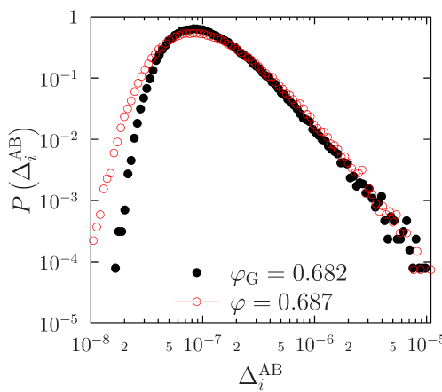
It is well known that, at the jamming point in finite dimensions, not all particles are part of the mechanically rigid network. Particles that are excluded from this network rattle relatively freely within their empty pores, hence the name “rattlers”. Because these localized excitations are not included in the infinite-dimensional theory, one could wonder whether the particles destined to become rattlers at jamming might play a role in our determination of the Gardner transition at finite dimensions. We argue here that it is not the case. Indeed, as shown in previous studies (see e.g. [38]), the effect of rattlers becomes important only for reduced pressure . The Gardner line detected in this work covers much lower reduced pressures, , which allows us to ignore rattlers.
Further support for this claim can be obtained by considering the probability distribution function of individual particle cage sizes calculated from many samples (with the thermal averaging) at the Gardner point and above it (Fig. 9), for one of the densest . Both distributions show a single peak with a power-law tail (which is consistent with previous work [39]). If rattlers gave a second peak, then they should be removed in our analysis, but this is not the case here.
Appendix E Caging timescale
We define a timescale to characterize the onset of caging. The ballistic regime of MSD at different is described by a master function , independent of waiting time , where the microscopic parameters and correspond to the peak of the MSD (see Fig. 10a). To remove the oscillatory peak induced by the finite system size, we introduce slightly larger than, but proportional to , so that corresponds to the beginning of the plateau. The same collapse is obtained for any ; as a result, is independent of . Above , is the time needed for relaxing the fastest vibrations. The dependence of on is summarized in Fig. 10b. Note that with weak variation for all considered state points.
By contrast, the mean-squared distance between two copies, , depends only weakly on (see Fig. 2b in the main text). Our choice of therefore does not affect substantially the value of (Fig. 3 in the main text). Note that, basically describes the asymptotic long time behavior of , i.e, .
Appendix F Absence of crystallization and of thermodynamic anomalies at the Gardner density
It is quite obvious that, because the system is not diffusing away from the original liquid configuration at during the simulation time window, no crystallization can happen in the glass regime. Indeed, when crossing no sign of incipient crystallization or formation of comparable anomaly appears in the pair correlation function. Also, is essentially constant in the glass regime; nothing special happens to this quantity at . The crossover would thus remain invisible if we only considered the compressibility and not more sophisticated observables.
Appendix G Time evolution of and timescales
The relaxation timescale (Fig. 2d in the main text) was extracted from fitting the long-time behavior of to a logarithmic scaling formula , following the strategy discussed in previous works [11, 40]. This particular choice of functional form makes it easier to obtain reliable fits for the whole window of parameters and . A more conventional scaling function, such as
| (8) |
has a stronger theoretical motivation, but at the cost of requiring more fitting constants. Data is nonetheless also well described by this functional form, as we show in Fig. 11a, where the solid lines are obtained from fits to the functional form Eq. (8) and the dashed lines are the logarithmic fits from Fig. 2c in the main text.
One can also fit Eq. (8) to extract a new estimate of the timescale . If doing so, we obtain results essentially proportional to our previous estimate of (Fig. 11b). In this sense, both scalings appear to be equivalent (at least for low and where both fits can be done). More quantitatively, one can also attempt a fit of the two characteristic times to a power-law divergence,
| (9) |
as is expected in the vicinity of a critical point (Fig. 11b). Again, we obtain values within the error bars of the parameters. In particular, and , which is completely compatible with our best estimate for the Gardner point, , at this .
MCT further suggests that there should be a relation between the exponent obtained from the fit of Eq. (9) and the exponent from the fit of Eq. (8). At this point, we could not fit the data using a constant value of for all densities. Instead, the exponent decreases as increases (see Fig. 11c), and becomes increasingly incompatible with extracted from the fit Eq. (9). Although this fact seems to be inconsistent with the mean-field theory, the same behavior of (also quantitatively) was recently reported in a similar study in a mean-field model of hard spheres (HS) over comparable timescales [11]. This inconsistency might thus be related to the inner technical difficulty of fitting the exponent using Eq. (8).
Appendix H Time dependence of the skewness and determination of the Gardner density
In this section, we explicitly show that the position of the peak of the skewness , which is used to extract the location of the Gardner point (Fig. 3d in the main text), is independent of the choice of timescale, . Promoting the skewness to a time-dependent quantity, , with , confirms that the peak position of is nearly invariant of , although the peak height does have a small time dependence.
Appendix I System-size dependence of the susceptibility at the Gardner transition
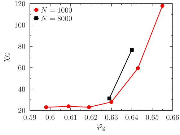
From a theoretical viewpoint, whether the mean-field Gardner transition persists in finite dimensions is still under debate [37]. In this work, we have shown the existence of a crossover (reminiscent of the mean-field Gardner transition) at two system sizes, and . However, the proof of the existence of the Gardner transition in the thermodynamic limit would require a systematic use of finite-size scaling techniques [41], which is beyond the scope of this paper. Previous studies further suggest that this kind of analysis might be extremely challenging. For example, symmetry arguments suggest that the Gardner transition should be in the same universality class as the de Almeida-Thouless line in mean-field spin-glasses in a field [37], whose finite-dimensional persistence is still the object of active debate even after intensive numerical scrutiny [42, 43, 44, 45]. One way to test whether our data are compatible with a true phase transition is by checking that the caging susceptibility at the transition point, , appears to divergence at . Considering that must be finite in a finite system (as shown it Fig. 3c for ), the divergence requires that increases with . We can see that this requirement is fulfilled in Fig. 13, which compares susceptibilities for and 8000.
Appendix J Compression-Rate Dependence
In this section, we consider how our overall analysis depends on the compression rate used for preparing samples. In principle, a proper should be such that particles have sufficient time to equilibrate their vibrations but not to diffuse. In other words, the timescale associated with compression, , should lie between the and relaxation times, . For our system, we observe that when and , both and reach flat plateaus that are essentially independent of (see Figs. 14a and b). Thus in this range of compression rates, restricted equilibrium within a glass state is reached, while keeping the relaxation sufficiently suppressed. When , however, and display -dependent aging effects consistent with a growing timescale in the Gardner phase. As a result, the order parameters and , which are defined at the time scale of , slightly depend on when (see Fig. 14c). This mild -dependence has nonetheless relatively little impact on our analysis of . In particular, the location of the peak position of the caging skewness, based on which we determine the value of , is independent of within the numerical accuracy (see Fig. 14d). Note that plays a role akin to the waiting time . Varying is thus equivalent to varying (see Fig. 2a and Fig. 14a).
Appendix K Spatial correlation functions and lengths
In this section, we provide a more detailed presentation of the spatial correlations of individual cages and of their associated length scales. We consider both point-to-point and line-to-line spatial correlation functions, and show that the characteristic lengths obtained from both grow consistently around . We also highlight the advantage of the line-to-line correlation function, which is used in the main text. Note that the results presented here are all for , while in the main text results for the line-to-line correlation are reported for .
The susceptibility discussed in the main text is directly associated with the unnormalized point-to-point spatial correlation function computed between two copies, and ,
| (10) |
This definition gives . Because in an isotropic fluid is a rotationally invariant function, we define the normalized radial correlation
| (11) |
where and the denominator is essentially the pair-correlation function between two clones,
| (12) |
In a similar way, we define the normalized line-to-line spatial correlation function
| (13) |
where is the projection of the particle position along the direction . This last definition is also Eq. (6) in the main text.
Both spatial correlation functions should capture the growth of vibrational heterogeneity around and are expected to decay at long distances as
| (14) |
where the damping function, , could in principle be different at large for and . The function is normally assumed to have an exponential or a stretched exponential form [46]. Equation (14) suggests that , which means that the observed growth in around (Fig. 3c in the main text) should also be observed for , but with a different exponent.
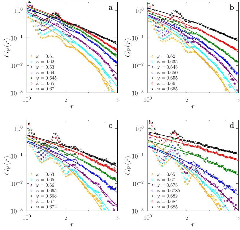
Although is the commonly used spatial correlation function, we find that traditionally used in lattice field theories [47] is more convenient to extract . To illustrate why, we plot in Fig. 15 and in Fig. 16 for different . Compared to , the line-to-line correlation function has the following advantages: (i) oscillations at small are removed, which better reveals the power-law scaling ; (ii) it is easier to incorporate the periodic boundary condition by simply adding a symmetric term to (7), where is the linear size of the system; and (iii) the tail of decays faster than that of , which implies a better separation between the power-law regime, , and the tail, . The tail of is indeed well described by a stretched exponential, while has a slower exponential decay.
(a) (b)
(c) (d)
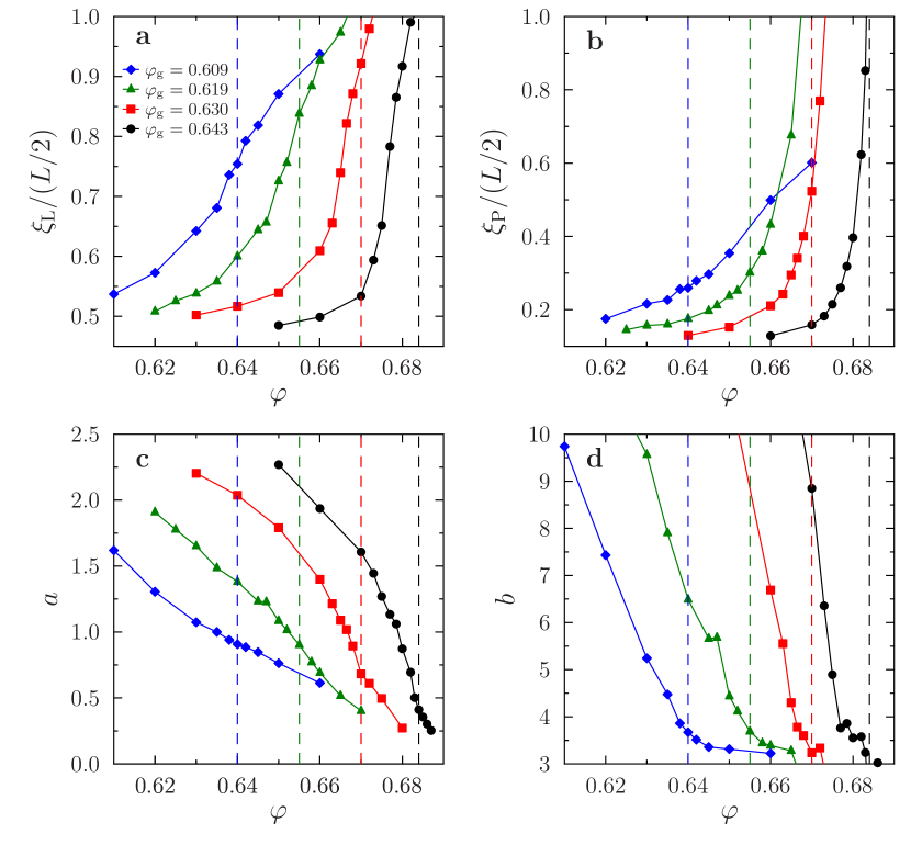
We extract from fitting at different (see Fig. 17a) to the functional form
| (15) |
These fits also allow us to extract the exponents and , which we find to have a strong dependence on , as shown in Fig. 17c and d. The oscillations of at low values of , however, make impossible an accurate extraction of from fitting. For this reason, we impose (an intermediate value of in Fig. 17c) and , and extract from fitting to
| (16) |
The results for this second correlation length are shown in Fig. 17b. Both estimators are expected to measure the same object, that is, both and should be proportional to the true correlation length, . The actual values obtained from both fits must, however, be regarded merely as indicators of the correlation growth, because the extraction of is rather inaccurate. The linear size of simulation box should be several times larger than the correlation length to obtain accurate estimations.
The growth in the heterogeneity of the system can be visualized by looking at the spatial fluctuations of . Figure 18 shows the typical cages of all the particles at different along the compression process. The cage of particle () is represented as a sphere of diameter centered in . The normalization fixes the average cage size, , for the sake of visualization.
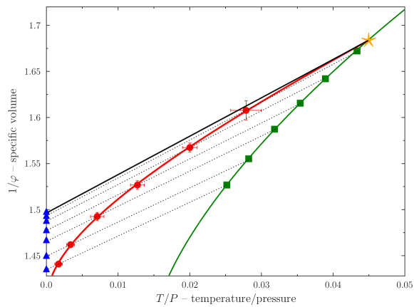
Appendix L Phase diagram for thermal glasses
In order to connect our phase diagram for HS (Fig. 1 in the main text) with traditional presentations of thermal glass results (see, e.g, Fig. 1 in Ref. [48]), we present an alternate version of that phase diagram (Fig. 19). In this different representation, we plot the specific volume as the axis and the ratio between temperature and pressure as the axis. It essentially describes how the specific volume changes with the temperature, at constant pressure, in different phases. We expect this phase diagram to be qualitatively reproducible in thermal glass experiments.
Appendix M Bidisperse hard disk results and analysis
We also study a two-dimensional bidisperse model glass former [49], using the same approach as for HS described the main text. The system consists of an equimolar binary mixture of hard disks (HD) with diameter ratio . In this case, we do not use the swap algorithm. Equilibrium configurations are obtained by slow relaxations during MD runs, so that particles all diffuse, i.e., . For each , samples are obtained. The liquid EOS is fitted to
| (17) |
where
| (18) |
is the 2 Carnahan-Starling (CS) form, and
| (19) |
is a fitted function with parameters , , , and . The estimated dynamical crossover is . The version of is obtained from the peak of caging skewness of big particles. The results are summarized in Table 2 and the phase diagram is reported in Fig. 20.
Appendix N Summary of numerical results
| 0.598 | 0.670(1) | 0.622(4) |
| 0.609 | 0.672(1) | 0.638(2) |
| 0.619 | 0.677(1) | 0.655(2) |
| 0.630 | 0.682(1) | 0.670(2) |
| 0.643 | 0.690(1) | 0.684(1) |
| 0.655 | 0.697(1) | 0.694(1) |
| 0.792 | 0.852(1) | 0.815(5) |
| 0.796 | 0.853(1) | 0.830(2) |
| 0.80 | 0.855(1) | 0.835(2) |
| 0.804 | 0.856(1) | 0.843(2) |
| 0.808 | 0.857(1) | 0.847(2) |
References
- [1] Berthier L, Biroli G (2011) Theoretical perspective on the glass transition and amorphous materials. Rev. Mod. Phys. 83:587–645.
- [2] Cavagna A (2009) Supercooled liquids for pedestrians. Phys. Rep. 476:51–124.
- [3] Phillips WA (1987) Two-level states in glasses. Rep. Prog. Phys. 50:1657.
- [4] Goldstein M (2010) Communications: Comparison of activation barriers for the Johari–Goldstein and alpha relaxations and its implications. J. Chem. Phys. 132:041104.
- [5] Malinovsky VK, Sokolov AP (1986) The nature of boson peak in Raman scattering in glasses. Solid State Commun. 57:757–761.
- [6] Hentschel HGE, Karmakar S, Lerner E, Procaccia I (2011) Do athermal amorphous solids exist? Phys. Rev. E 83:061101.
- [7] Müller M, Wyart M (2015) Marginal stability in structural, spin, and electron glasses. Annu. Rev. Condens. Matter Phys. 6:177–200.
- [8] Wolynes P, Lubchenko V, eds (2012) Structural Glasses and Supercooled Liquids: Theory, Experiment, and Applications (Wiley).
- [9] Charbonneau P, Kurchan J, Parisi G, Urbani P, Zamponi F (2014) Fractal free energy landscapes in structural glasses. Nat. Comm. 5:3725.
- [10] Gardner E (1985) Spin glasses with -spin interactions. Nuclear Physics B 257:747–765.
- [11] Charbonneau P, et al. (2015) Numerical detection of the Gardner transition in a mean-field glass former. Phys. Rev. E 92:012316.
- [12] Grigera TS, Parisi G (2001) Fast Monte Carlo algorithm for supercooled soft spheres. Phys. Rev. E 63:045102.
- [13] Boublik T (1970) Hard sphere equation of state. J. Chem. Phys. 53:471.
- [14] Russo J, Tanaka H (2015) Assessing the role of static length scales behind glassy dynamics in polydisperse hard disks. Proceedings of the National Academy of Sciences 112:6920–6924.
- [15] Flenner E, Szamel G (2015) Fundamental differences between glassy dynamics in two and three dimensions. Nature communications 6.
- [16] Berthier L, Coslovich D, Ninarello A, Ozawa M (2015) Equilibrium sampling of hard spheres up to the jamming density and beyond. arXiv preprint arXiv:1511.06182.
- [17] Yaida S, Berthier L, Charbonneau P, Tarjus G (2015) Point-to-set lengths, local structure, and glassiness. arXiv preprint arXiv:1511.03573.
- [18] Charbonneau P, Jin Y, Parisi G, Zamponi F (2014) Hopping and the Stokes–Einstein relation breakdown in simple glass formers. Proc. Natl. Acad. Sci. U.S.A. 111:15025–15030.
- [19] Chaudhuri P, Berthier L, Sastry S (2010) Jamming transitions in amorphous packings of frictionless spheres occur over a continuous range of volume fractions. Phys. Rev. Lett. 104:165701.
- [20] Ozawa M, Kuroiwa T, Ikeda A, Miyazaki K (2012) Jamming transition and inherent structures of hard spheres and disks. Phys. Rev. Lett. 109:205701.
- [21] Skoge M, Donev A, Stillinger FH, Torquato S (2006) Packing hyperspheres in high-dimensional Euclidean spaces. Phys. Rev. E 74:041127.
- [22] Parisi G, Rizzo T (2013) Critical dynamics in glassy systems. Phys. Rev. E 87:012101.
- [23] Berthier L, Biroli G, Bouchaud JP, Cipelletti L, van Saarloos W, eds (2011) Dynamical Heterogeneities and Glasses (Oxford University Press).
- [24] Cohen Y, Karmakar S, Procaccia I, Samwer K (2012) The nature of the -peak in the loss modulus of amorphous solids. Europhys. Lett. 100:36003.
- [25] Bock D, et al. (2013) On the cooperative nature of the -process in neat and binary glasses: A dielectric and nuclear magnetic resonance spectroscopy study. J. Chem. Phys. 139:064508.
- [26] Leheny RL, Nagel SR (1998) Frequency-domain study of physical aging in a simple liquid. Phys. Rev. B 57:5154.
- [27] Brito C, Wyart M (2009) Geometric interpretation of previtrification in hard sphere liquids. J. Chem. Phys 131:024504.
- [28] Rössler E, Sokolov A, Kisliuk A, Quitmann D (1994) Low-frequency Raman scattering on different types of glass formers used to test predictions of mode-coupling theory. Phys. Rev. B 49:14967.
- [29] Velikov V, Borick S, Angell CA (2001) The glass transition of water, based on hyperquenching experiments. Science 294:2335.
- [30] Swallen SF, et al. (2007) Organic glasses with exceptional thermodynamic and kinetic stability. Science 315:353–356.
- [31] Singh S, Ediger MD, de Pablo JJ (2013) Ultrastable glasses from in silico vapour deposition. Nat. Mater. 12:139–144.
- [32] Hocky GM, Berthier L, Reichman DR (2014) Equilibrium ultrastable glasses produced by random pinning. J. Chem. Phys. 141.
- [33] Pérez-Castañeda T, Rodríguez-Tinoco C, Rodríguez-Viejo J, Ramos MA (2014) Suppression of tunneling two-level systems in ultrastable glasses of indomethacin. Proc. Nat. Acad. Sci. U.S.A. 111:11275–11280.
- [34] Liu X, Queen DR, Metcalf TH, Karel JE, Hellman F (2014) Hydrogen-free amorphous silicon with no tunneling states. Phys. Rev. Lett. 113:025503.
- [35] Yu HB, Tylinski M, Guiseppi-Elie A, Ediger MD, Richert R (2015) Suppression of relaxation in vapor-deposited ultrastable glasses. Phys. Rev. Lett. 115:185501.
- [36] Hu X, et al. (2015) The dynamics of single protein molecules is non-equilibrium and self-similar over thirteen decades in time. Nat. Phys. 12:171–174.
- [37] Urbani P, Biroli G (2015) Gardner transition in finite dimensions. Phys. Rev. B 91:100202.
- [38] Charbonneau P, Corwin EI, Parisi G, Zamponi F (2012) Universal microstructure and mechanical stability of jammed packings. Phys. Rev. Lett. 109:205501.
- [39] Maiti M, Sastry S (2014) Free volume distribution of nearly jammed hard sphere packings. The Journal of chemical physics 141:044510.
- [40] Baity-Jesi M, et al. (2014) Dynamical transition in the d= 3 edwards-anderson spin glass in an external magnetic field. Phys. Rev. E 89:032140.
- [41] Amit DJ, Martin-Mayor V (2005) Field theory, the renormalization group, and critical phenomena (World Scientific Singapore) Vol. 3rd ed.
- [42] Young A, Katzgraber HG (2004) Absence of an almeida-thouless line in three-dimensional spin glasses. Physical review letters 93:207203.
- [43] Larson D, Katzgraber HG, Moore M, Young A (2013) Spin glasses in a field: Three and four dimensions as seen from one space dimension. Physical Review B 87:024414.
- [44] Baity-Jesi M, et al. (2014) The three-dimensional ising spin glass in an external magnetic field: the role of the silent majority. Journal of Statistical Mechanics: Theory and Experiment 2014:P05014.
- [45] Baños RA, et al. (2012) Thermodynamic glass transition in a spin glass without time-reversal symmetry. Proceedings of the National Academy of Sciences 109:6452–6456.
- [46] Belletti F, et al. (2008) Nonequilibrium spin-glass dynamics from picoseconds to a tenth of a second. Phys. Rev. Lett. 101:157201.
- [47] Rothe HJ (2005) Lattice gauge theories: an introduction (World Scientific) Vol. 74.
- [48] Debenedetti PG, Stillinger FH (2001) Supercooled liquids and the glass transition. Nature 410:259.
- [49] Berthier L (2014) Nonequilibrium glassy dynamics of self-propelled hard disks. Phys. Rev. Lett. 112:220602.