Strong quantum scarring by local impurities

Abstract

We discover and characterize strong quantum scars, or eigenstates resembling classical periodic orbits, in two-dimensional quantum wells perturbed by local impurities. These scars are not explained by ordinary scar theory, which would require the existence of short, moderately unstable periodic orbits in the perturbed system. Instead, they are supported by classical resonances in the unperturbed system and the resulting quantum near-degeneracy. Even in the case of a large number of randomly scattered impurities, the scars prefer distinct orientations that extremize the overlap with the impurities. We demonstrate that these preferred orientations can be used for highly efficient transport of quantum wave packets across the perturbed potential landscape. Assisted by the scars, wave-packet recurrences are significantly stronger than in the unperturbed system. Together with the controllability of the preferred orientations, this property may be very useful for quantum transport applications.

Quantum scars Kaplan (1999) are enhancements of probability density in the eigenstates of a quantum chaotic system that occur around short unstable periodic orbits (POs) of the corresponding classical system. Scars have been observed experimentally in, e.g., microwave cavities Sridhar (1991); *stein, optical cavities Lee et al. (2002); *harayama, and quantum wells Fromhold et al. (1995); *wilkinson, and computationally in, e.g., simulations of graphene flakes Huang et al. (2009) and ultracold atomic gases Larson et al. (2013).

Before the existence of scars was reported by Heller Heller (1984), eigenstates of a classically chaotic system were conjectured to fill the available phase space evenly, up to random fluctuations and energy conservation. If high-energy eigenstates of non-regular (i.e., generic) systems were indeed featureless and random, controlled applications in that regime would be difficult. Scars are therefore both a striking visual example of classical-quantum correspondence away from the usual classical limit, and a useful example of a quantum suppression of chaos.

In this work we describe quantum scars present in otherwise separable systems disturbed by local perturbations such as impurity atoms. In this case, scars are formed around POs of the corresponding unperturbed system. These scars are significantly stronger than what ordinary scar theory predicts, which we explain by introducing a new scarring mechanism.

In the following, values and equations are given in natural units where the quantum Hamiltonian is simply $H=-\tfrac{1}{2}\nabla^{2}+V+V_{\text{imp}}$, where $V$ is the unperturbed potential and $V_{\text{imp}}$ represents the perturbation.

I Model system

The scarring mechanism, explained later in this Letter, is very general; it requires only that the unperturbed system is separable, and that the perturbing impurities are sufficiently local. In the following we focus, for simplicity, on a few prototypical examples of a circularly symmetric, two-dimensional potential well $V(r)$ perturbed by randomly scattered Gaussian bumps.

The classical POs of any circularly symmetric $V(r)$ can be enumerated directly (see Supplementary Material and Ref. Reynolds and Shouppe (2010)). Each PO is associated with a resonance, where the oscillation frequencies of the radial and angular motion are commensurable. The PO structure is especially simple if $V(r)$ is a homogeneous function (i.e., $V(r)\propto r^{a}$), since then POs with different total energies differ only by a scaling.

In the following we use $a=5$. Its shortest non-trivial PO is a five-pointed star, which is both easily distinguishable and short. This PO corresponds to a $2\!:\!5$ classical resonance, where the orbit circles the origin twice in the time of five radial oscillations. The case of $a=2$, the harmonic oscillator, is special and ill-suited for drawing general conclusions, while for $a=1,3,4$ the shortest non-trivial POs are longer.

For easier comparison between the results, we focus in the following on a single example shown in Fig. 1(a), where Gaussian bumps with amplitude $M=24$ are distributed in an unperturbed potential $V(r)=\frac{1}{2}r^{5}$. The average density of the bumps is two per unit square, and thus for a typical energy of $500$, approximately a hundred bumps exist in the classically allowed region. The full width at half maximum (FWHM) of the Gaussian bumps is $0.235$, which is similar to the typical local wavelength of the eigenstates we consider.

The amplitude of the bumps is small compared to the total energy, making each individual bump a small perturbation. Nevertheless, together the impurities are sufficient to destroy classical long-time stability; any stable structures present in the otherwise chaotic Poincaré surface of section are tiny compared to $\hbar=1$.

II Scar observations

Figure 1(b) shows an example of a scar found in the eigenstates of the example potential described previously. The eigenstates are solved with imaginary time propagation in real space Luukko and Räsänen (2013). Figures 1(c)–(e) show examples of scars in a homogeneous potential with exponent $a=8$, and in a non-homogeneous potential $V(r)\propto\cosh(r)-1$. In all cases the scars follow POs in the corresponding unperturbed system. We note that the scars are not a rare occurrence; for the potential in Fig. 1(a) over 10% of the eigenstates are clearly scarred. The scars are also very strong; in Fig 1(b) approximately 80% of the probability density resides on the star path.

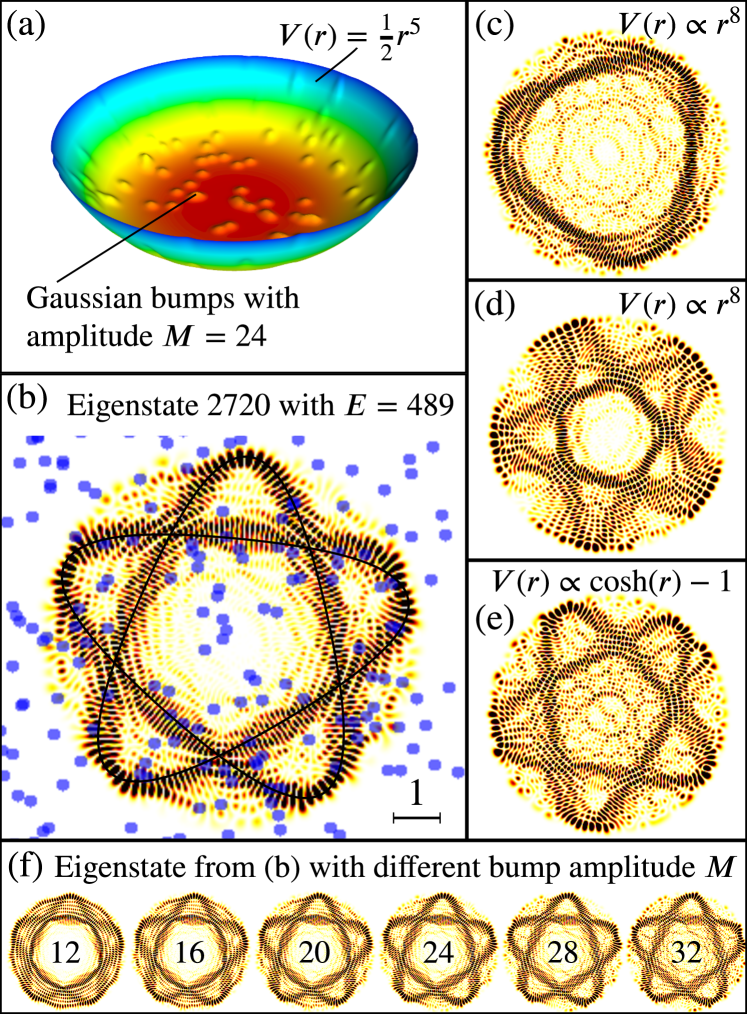
Figure 1: Examples of scarred eigenstates in perturbed potential wells. An example potential well $V(r)=\tfrac{1}{2}r^{5}$ perturbed by Gaussian bumps is shown in (a) and one of its strongly scarred eigenstates is shown in (b). Blue markers denote the locations and full widths at half maximum of the bumps, and the corresponding PO of the unperturbed potential is drawn as a solid line. Note that several bumps are located on the scar path. Examples of scars in other potentials are shown in (c)–(e). The eigenstate in (b) at different bump amplitudes $M$ is shown in (f). The scar shape and orientation remain unchanged as $M$ increases.

In ordinary scar theory Heller (1984), each scar corresponds to a moderately unstable PO in the classical system. In this case such orbits do not exist. For example, the shortest and least unstable PO near the scar shown in Fig. 1(f) for $M=16$ closes on itself after two rounds around the scar, and has a one-period stability exponent Gutzwiller (1990) $\chi\approx 5$. This is by far too unstable to cause a conventional scar as strong.

Ordinary scar theory is also excluded by the behavior of the scars as a function of the bump amplitude $M$. If $M$ is increased while keeping $V_{\text{imp}}$ otherwise unchanged, the scars grow stronger and then fade away without changing their orientation, as shown in Fig. 1f. A scar caused by ordinary scar theory should become rapidly weaker, since the stability exponent of a PO should increase with $M$.

Comparing scars at different energies $E$ reveals that they occur in only a few distinct orientations, and these orientations change quite slowly with $E$ (see Fig. 3). For the example $V_{\text{imp}}$ used here there are three preferred orientations. For other impurity realizations the number and location of the preferred orientations vary (see Supplementary Material), but the existence of preferred scar orientations is a generic feature. This too contradicts predictions of ordinary scar theory.

III Wave-packet analysis

Gaussian wave packets are a standard tool for studying eigenstate scarring Heller (1984). If a Gaussian wave packet $|\phi\rangle$ is centered on a scarring PO, its autocorrelation function $A(t)=\langle\phi(0)|\phi(t)\rangle$ shows clear short-time recurrences with a period $T$ matching the period of the PO. In ordinary scarring the strength of these recurrences $|A(nT)|^{2}$ dies out as $1/\cosh(\chi n)$, where $\chi$ is the stability exponent of the PO Kaplan and Heller (1999). In addition, $|\langle\phi(0)|\psi\rangle|$ is large for an eigenstate scarred by the particular PO, making wave packets useful for detecting scarred eigenstates.

In our case we use the PO of the unperturbed system to initialize the wave packet. The energy and the orientation of the PO are matched to the scarred eigenstate. The width parameters of the Gaussian are matched approximately to the geometry of the scar (see the inset in Fig. 2).

The wave packets selected in this way have a considerable energy uncertainty, so that many scars, sharing the same approximate orientation, contribute to the recurrences. A typical FWHM of the wave packet is approximately $50$ energy units, or $400$ eigenstates.

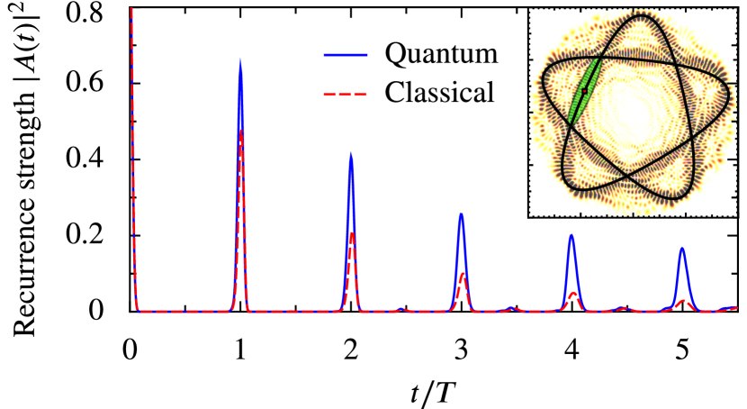
Figure 2: Recurrence strength of a Gaussian wave packet propagating along the scar in Fig. 1b. The quantum recurrence strength (solid blue line) is compared with the corresponding classical recurrence strength (dashed red line). Time is shown in units of the period $T$ of the unperturbed PO. The scar, the corresponding PO (solid black line) and the location and full width at half maximum of the initial Gaussian (green area) are shown in the inset.

Figure 2 shows the recurrence strength $|A(t)|^{2}$ for a wave packet traveling on the scar shown in Fig. 1(b). Clear periodic recurrences are visible, with a period that matches the period of the unperturbed PO.

To account for purely classical effects, we compare the results with the recurrence of the corresponding classical density . The classical recurrences are significantly weaker than the quantum recurrences even at $t=T$, and this difference grows rapidly at later times, illustrating the quantum nature of the phenomenon.

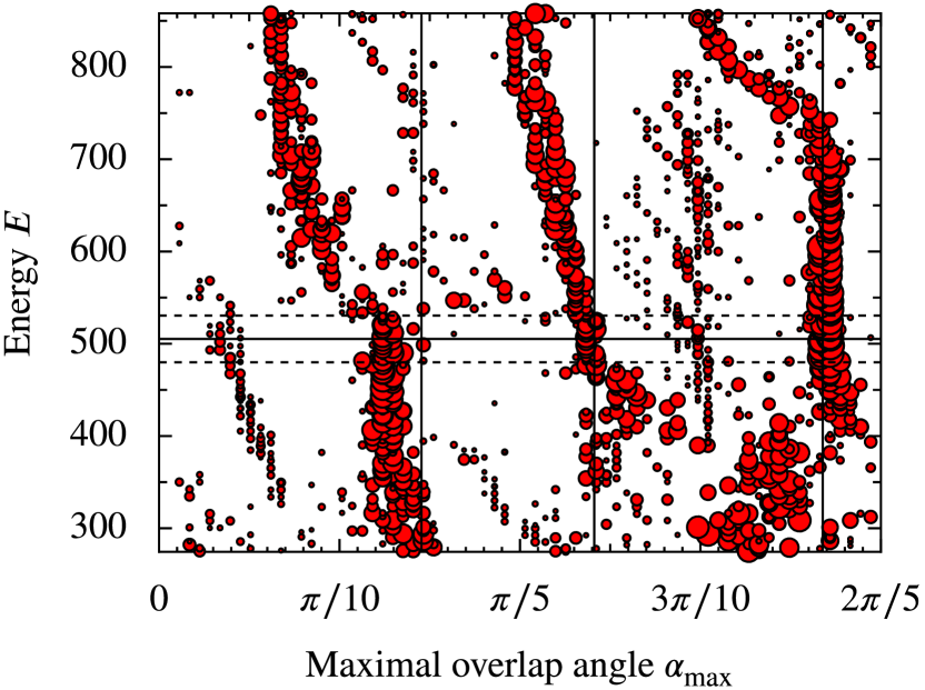
Figure 3: Scatter plot demonstrating the existence and stability of the preferred scar orientations. For each eigenstate, a circle is marked on the orientation angle $\alpha$ showing the highest overlap between the eigenstate and an initial Gaussian wave packet with the given orientation. The radius of the circle gives its squared magnitude. Squared overlaps of less than $3\cdot 10^{-3}$ are excluded. The vertical coordinate is the common energy of the eigenstate and the PO. The solid and dashed horizontal lines show, respectively, the mean energy and energy FWHM of the wave packet used in Fig. 2. For easier comparison, orientation angles with peaks at $t=4T$ in Fig. 4, are marked with solid vertical lines.

The existence of stable preferred scar orientations can be demonstrated by systematically detecting scarred states with wave packets. Figure 3 shows how the overlap of the initial wave packet with the target eigenstate depends on the energy of the eigenstate and the orientation of the PO used to initialize the wave packet. The orientation coordinate $\alpha$ is such that at $\alpha=0$ the wave packet starts on the positive $y$-axis and heads to the right.

In an angular window of $2\pi/5$ (after which the PO is the same), three branches of high overlaps are visible, corresponding to the preferred orientations. Note that the rightmost branch is roughly vertical for $E=400\dotsc 700$, corresponding to an increase of the average radius of the PO by roughly $0.3$ units, which is the length scale of the individual bumps.

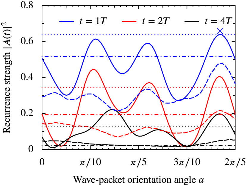
Figure 4: Amplitude of recurrence peaks shown in Fig. 2 as a function of the initial wave packet orientation $\alpha$. Solid lines and dashed lines show the quantum and classical results, respectively. Dash-dotted and dotted lines show the quantum and classical results in the unperturbed system, respectively. Blue, red, and black lines correspond to snapshots after one, two, and four periods, respectively. The orientation angle used in Fig. 2 is marked with a blue cross. This is also the orientation that matches the scar shown in Fig. 1(b).

Figure 4 shows how the amplitude of the recurrence peaks in Fig. 2 depend of the orientation angle $\alpha$. Both quantum and classical wave-packets show stronger short-time recurrences at the preferred orientations, indicating that the preferred orientations can also be explained classically. However, especially at the preferred orientations, quantum late-time recurrences are much stronger than in the classical case.

Note that the quantum recurrences are stronger than the classical ones even on average, suggesting that there is also an effect that strengthens quantum recurrences at all orientations.

To highlight how strong the quantum recurrences are, a comparison to recurrences in the unperturbed system is also shown in Fig. 4. For the preferred orientations, the quantum late-time recurrences greatly exceed the strength of both the quantum and the classical recurrences in the unperturbed system. Via the creation of strong scars with stable preferred orientations, the randomly scattered impurities enhance the coherent propagation of quantum wave packets in the potential well!

IV Perturbation theory

Both the existence of scars and the preferred orientations can be explained by perturbation theory. This explanation is based on two ingredients. Firstly, special nearly-degenerate subspaces exist in the basis of unperturbed eigenstates. Secondly, the local perturbations select scarred eigenstates from these subspaces.

The eigenstates of the unperturbed, circularly symmetric system are labeled by two quantum numbers $(r,m)$, corresponding to radial and angular motion, respectively. States $(r,\pm m)$ are exactly degenerate, but in addition there are near-degeneracies that correspond to classical POs.

By the Bohr–Sommerfeld quantization condition (a good approximation at high quantum numbers) the energy difference from increasing $r$ or $m$ by one is proportional to the classical oscillation frequency of the corresponding action. Thus, if a state $(r,m)$ is nearby in action to a classical PO with a ratio $a\!:\!b$ between the oscillation frequencies, the state $(r+a,m-b$) will be nearby in energy. The smaller $a$ and $b$ are the closer the near-degeneracy is. This creates “resonant sets” of unperturbed basis states, and a part of a resonant set can be almost degenerate. Expanding in the unperturbed basis reveals that the scarred eigenstates are localized to such near-degenerate subspaces.

A superposition of two resonant states will exhibit beating in both the radial and angular directions. Because the ratio of the beat frequencies is also $a\!:\!b$, the interference pattern will trace out the shape of the classical PO. Adding more resonant states with appropriate phases will narrow the region of constructive interference and sharpen the scar, and even a few basis states can create a distinctly classical-looking linear combination. Similar reconstruction of classical-like states from (nearly) degenerate basis states has also been studied previously Liu et al. (2006); *squarelocalization; *ripple; *pollet. However, to create strongly scarred eigenstates with preferred orientations a mechanism that favors these scarred linear combinations is required.

Within the impurity strength regime that results in the strongest scarring, the perturbation $V_{\text{imp}}$ mostly only couples resonant, near-degenerate basis states. This locality is enhanced by the rapid weakening of the coupling with increasing difference in quantum numbers between the states. One can therefore approximate the perturbed eigenstates by degenerate perturbation theory (DPT), i.e., by diagonalizing $V_{\text{imp}}$ within the near-degenerate subspace.

The DPT-produced eigenstates corresponding to the extremal eigenvalues of $V_{\text{imp}}$ are, by the variational principle, the states $|\psi\rangle$ that extremize the expectation value $\langle V_{\text{imp}}\rangle\coloneqq\langle\psi|V_{\text{imp}}|\psi\rangle$. This quantity for a non-scarred, spatially delocalized state is essentially an average value of $V_{\text{imp}}$ over the entire accessible region, and never an extremum. Compared to the non-scarred states, the scarred states in a near-degenerate subspace have their probability amplitude concentrated in a much smaller region of space. For a $V_{\text{imp}}$ consisting of local impurities the state that maximizes (minimizes) $\langle V_{\text{imp}}\rangle$ will therefore generally be a scarred state oriented so as to coincide with an anomalously many (few) impurities.

By the previous argument the scar orientations are mostly selected by the positions of the impurities. Since the inner and outer radii of the POs change slowly with energy, the orientations that extremize $\langle V_{\text{imp}}\rangle$ will be determined largely by the same impurities for many different resonant sets. This is the origin of the stability of the preferred orientations seen in Fig. 3.

Though a simple DPT approximation does not reproduce the true eigenstates exactly, it both explains the scarring and predicts the orientations of the observed scars well, as illustrated in Fig. 5. Taking into account the imperfect degeneracy amounts to diagonalizing the full Hamiltonian instead of only the perturbation Davydov (1976). This means that in the matrix that is diagonalized the diagonal elements are shifted by the (small) spacings of the near-degenerate basis states. This “quasi-DPT” (qDPT) approximation improves the agreement between the DPT approximation and the exact eigenstates, as shown in Fig. 5(b).

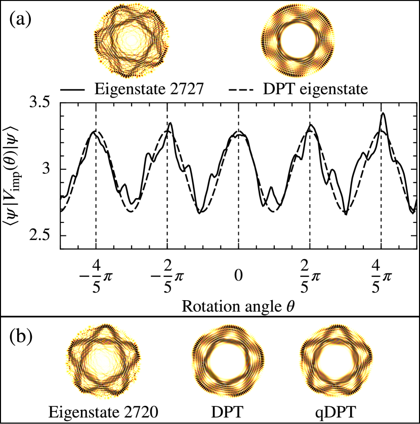
Figure 5: Reconstructing scarred eigenstates with degenerate perturbation theory (DPT). DPT reconstruction of a scarred eigenstate $2727$ is shown in (a). The plot depicts the expectation value $\langle V_{\text{imp}}(\theta)\rangle$, rotated by angle $\theta$ from the original $V_{\text{imp}}$, for both the actual eigenstate (solid line) and the eigenstate as predicted by DPT (dashed line). The plot shows that the orientation of the scar is such that $\langle V_{\text{imp}}\rangle$ is maximized. The overlap between the true eigenstate and the DPT reconstruction is 56%. The DPT reconstruction is calculated from a resonant set of only three nearly degenerate basis state doublets. Similar reconstruction of the eigenstate $2720$, shown also in Fig. 1b, is shown in (b). The DPT reconstruction produces a scar, but not at exactly the correct orientation. An improved quasi-DPT approximation, which takes into account the imperfect degeneracy, corrects it. The overlap between the eigenstate and the reconstruction is 60% for DPT and 68% for qDPT. The DPT reconstruction uses three nearly degenerate doublets, while the qDPT reconstruction uses five.

V Summary and outlook

To summarize, we have shown that a new type of quantum scarring is found in separable systems perturbed by local impurities. The scars are very strong, and they tend to occur in discrete preferred orientations. This allows wave packets to propagate through the perturbed system with higher fidelity than in the unperturbed system.

The theoretical basis of the scarring is very general, requiring only classical resonances and local perturbations. Therefore the scarring should have consequences well beyond the simple models discussed here.

The implications of the enhanced wave packet recurrences for quantum transport will be an important area for future work. In an experiment, local perturbations similar to the ones used here could be generated by a conducting nanotip Bleszynski et al. (2007); *nanotip2; *nanotip3, selecting particular scar orientations and enhancing the local conductance in a controlled way.

Supplementary material for “”

Appendix A Solving the periodic orbits of a circularly symmetric potential in 2D

The solution of the equations of motion for a classical particle in a circularly symmetric potential $V(r)$ can be found in standard texts on classical mechanics (e.g., Chapter 3 in Ref. Goldstein (1980)), but we summarize it here. The total energy $E$ of the particle is the sum of kinetic and potential energy, which in polar coordinates reads (in units where mass $m=1$)

$$E=\tfrac{1}{2}\dot{r}^{2}+\frac{L^{2}}{2r^{2}}+V(r),$$ (1)

where $L$ is the angular momentum, which is also a constant of motion. Solving for $\dot{r}$ from Eq. (1) gives

$$\dot{r}=\pm\sqrt{2}\sqrt{E-V(r)-\frac{L^{2}}{2r^{2}}}.$$ (2)

Changing variables in Eq. (2) from time to polar angle $\phi$ (using $\dot{\phi}=L/r^{2}$) and inverting gives

$$\frac{\mathrm{d}\phi}{\mathrm{d}r}=\pm\frac{L}{r\sqrt{2r^{2}\left[E-V(r)\right]-L^{2}}}\coloneqq\pm\frac{L}{r\sqrt{f(r)}},$$ (3)

where the function inside the square root is denoted as $f$. Equation (3) can be conveniently integrated to give the polar angle $\phi$ as a function of the radial coordinate $r$.

Assuming that $V(r)$ is a potential well ($V(r)$ is monotonically increasing and larger than $E$ for large enough $r$) and that $L\neq 0$, the radius of the particle oscillates between two turning points $r=a$ and $r=b$, which can be solved from Eq. (2) by setting $\dot{r}=0$. Not surprisingly, these turning points are exactly where $\mathrm{d}\phi/\mathrm{d}r$ diverges, i.e., the zeros of $f$ in Eq. (3). Between these turning points the radial coordinate either monotonically increases or decreases, corresponding to the positive and negative solutions in Eq. (2).

When the particle completes one oscillation from $r=a$ to $r=b$ and back, the corresponding change in the polar angle (by integrating Eq. (3)) is

$$\Delta\phi=\int_{a}^{b}\frac{2L}{r\sqrt{f(r)}}.$$ (4)

Note that $\Delta\phi$ is completely specified by the form of the potential $V(r)$ and the values for $E$ and $L$. The particle eventually returns to its starting point, i.e., the orbit is periodic, exactly when $\Delta\phi$ is a rational multiple of $2\pi$. If $\Delta\phi=2\pi\frac{m}{n}$ for integer $n$ and $m$, after $n$ oscillations between the radial turning points, the particle has rotated around the origin $m$ times, returning exactly to its starting position with its original velocity, i.e., the classical oscillation frequencies are in $m\!:\!n$ resonance. If the orbit is not periodic, it is quasiperiodic.

Searching for periodic orbits (POs) for a given potential $V(r)$ and total energy $E$ can be done conveniently by looking for zeros of the function $g(E,L,n)\coloneqq\sin\left(\tfrac{1}{2}n\Delta\phi\right).$ This can be done by any standard root-finding method, using $L$ as the free variable, and some set of discrete choices for the integer $n$. This gives values of $L$ which correspond to a PO, and the integers $n$ and $m$, which give the shape of the orbit.

The procedure is especially simple if $V(r)$ is a homogeneous function of $r$. In this case different total energies differ only by a scaling factor in space and time, which means the PO shapes do not depend on $E$. Moreover, for $V(r)\propto r^{a}$ with integer $a$, the function $f$ in Eq. (3) is a polynomial, which makes it particularly easy to find the turning points for moderate values of $a$.

As an illustration, the shortest POs for some small integer values of $a$ are given in Table 1. Most importantly, the five-pointed star with $m/n=2/5$ appears at $a=5$, and the next jump to a simpler shortest PO occurs at $a=8$ with the birth of the triangle orbit with $m/n=1/3$. The POs of power-law potentials are also studied in a more indirect way in Ref. Reynolds and Shouppe (2010).

Table 1: Periodic orbits for $V(r)\propto r^{a}$ up to $n=15$. Table entries are aligned by $n$ to highlight how new PO shapes appear with increasing $a$.

$a$	Periodic orbits as values of $m/n$
1			4/7		5/9	6/11		7/13		8/15
2	1/2 (harmonic oscillator – a very special case)
3						5/11		6/13		7/15
4			3/7		4/9	5/11	5/12	6/13		7/15
5		2/5	3/7		4/9	5/11	5/12	{5, 6}/13		7/15
6		2/5	3/7	3/8	4/9	{4, 5}/11	5/12	{5, 6}/13	5/14	7/15
7		2/5	3/7	3/8	4/9	{4, 5}/11	5/12	{5, 6}/13	5/14	7/15
8	1/3	2/5	3/7	3/8	4/9	{4, 5}/11	5/12	{5, 6}/13	5/14	7/15
9	1/3	2/5	3/7	3/8	4/9	{4, 5}/11	5/12	{4, 5, 6}/13	5/14	7/15

Appendix B Extracting scars with a wave-packet “scarmometer”

As explained in the main article, for ordinary scars a wave packet initialized on a PO can be used to locate eigenstates that are scarred by that particular orbit, since the scarred eigenstates will have large overlaps with the wave packet. Similarly a wave packet initialized on a specific PO of the unperturbed system can be used to isolate scars with that particular orientation in the perturbed system. This is illustrated in Fig. 6, which uses the wave packet used in Fig. 2 to isolate scarred eigenstates with the same orientation as the $n=2720$ example scar used throughout the main article. This illustration also shows how several scarred eigenstates contribute to the recurrences of a single wave packet.

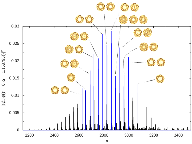
Figure 6: Extracting scars with a specific orientation with a wave packet “scarmometer”. The histogram in the background shows the basis decomposition of the wave packet used in Fig. 2 in the eigenstates of the perturbed system. Scarred eigenstates show up as prominent peaks in this decomposition. For some of the strongest peaks (marked in blue) the corresponding eigenstate is also shown, highlighting that they are all scarred to a varying degree, and that the orientation of the five-pointed scar is the same.

Appendix C Scars of other resonances in homogeneous potentials

The five-pointed star orbit in the $r^{5}$ potential is in some ways a natural “sweet spot” for scarring. The $2\!:\!5$ resonance produces tight near-degenerate resonant sets, because moving from one resonant state to the next involves the exchange of a small number of quanta, making the degeneracy approximation better.

The five-fold symmetry also gives more room for visually distinct preferred orientations, as opposed to, e.g., an 11-pointed star. Moreover, the existence of a self-crossing point in the classical orbit makes the probability density in a scar less uniform, which helps the localization of the scars as they will pin more strongly to impurities near the self-crossing point. This gives the five-pointed star some advantage over the two simpler resonances, $1\!:\!3$ and $1\!:\!4$.

In other homogeneous potentials, scarring due to classical resonances exists analogously to the $r^{5}$ case. With other choices of the exponent in the unperturbed potential, different resonances exist, as summarized in Table 1. This is reflected in the shape and abundance of scars. Figure 1 includes examples of scars in a $r^{8}$ potential.

The integer exponent $a=3$ is unusual in that its simplest non-trivial resonance is $5\!:\!11$. With coefficients so large the near-degeneracy in the resonant sets becomes poor, and the scars become rare and distorted. In fact, at this limit the near-degeneracy due to resonant sets might compete with purely accidental near-degeneracies. An even more extreme absence of short non-trivial classical resonances can be found with non-integer exponents close to $2$.

Appendix D Scars in a non-homogeneous potential

While a homogeneous potential function simplifies the classical PO structure, it is not necessary for scarring. Other forms of the unperturbed potential also have quasi-degenerate sets of eigenstates due to classical resonances, and thus local impurities will cause scars. Figure 1 contains an example of a five-pointed scar eigenstate for $V(r)\propto\cosh(r)-1$. In this case, the parameters of the perturbation are such that each Gaussian bump has amplitude $M=10$, FWHM of $0.353$, and the average density of bumps is $2.4$ bumps per unit square.

To provide more proof that similar scarring also exists for a non-homogeneous potential, Fig. 7 shows wave-packet recurrences as a function of the wave-packet orientation angle, and Fig. 8 shows eigenstates contributing to the recurrences of the strongest preferred orientation.

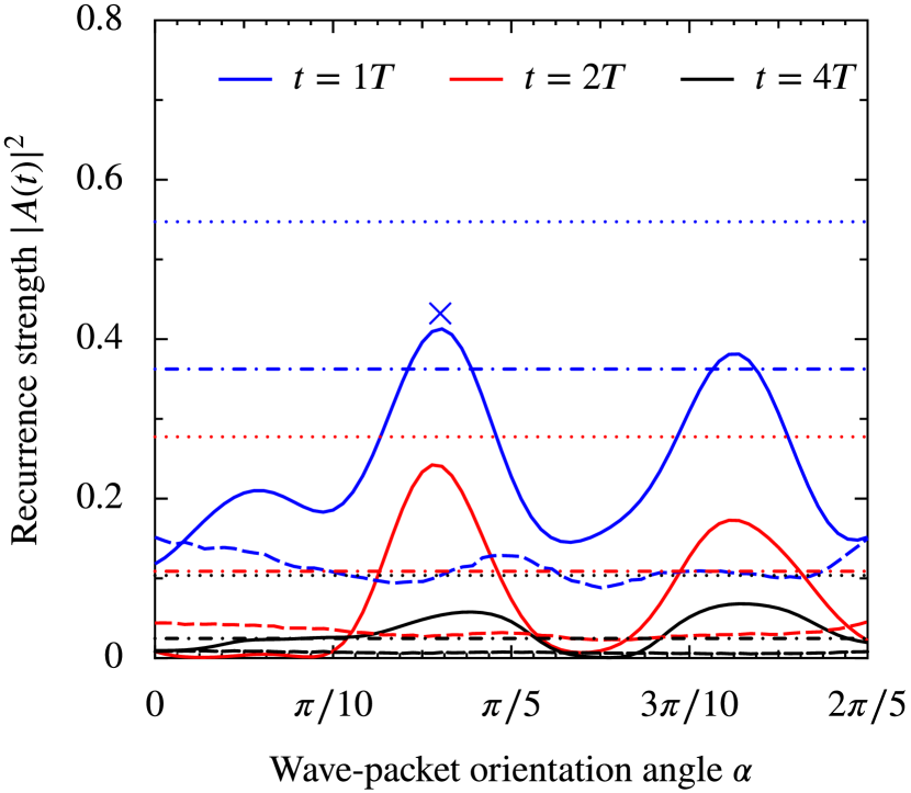
Figure 7: Plot equivalent to Fig. 4, except for a non-homogeneous unperturbed potential $V(r)\propto\cosh(r)-1$, with impurity parameters described in the text. The wave-packet was initialized on a $2\!:\!5$ PO with energy $E=200$.

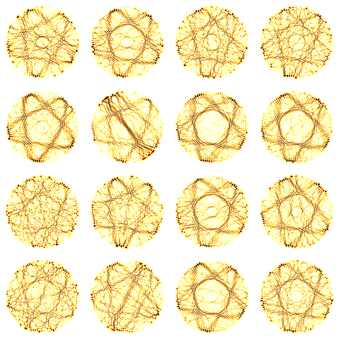
Figure 8: Most prominent eigenstates in the decomposition of the wave-packet in Fig. 7 at the most strongly recurring orientation (marked with a blue cross in Fig. 7).

Appendix E Generality of the results for different random realizations of the impurities

We have not attempted to specify quantitatively how common the scars or preferred orientations are among all random realizations of the impurity locations. To illustrate that they are not a rare occurrence by any means, Fig. 9 shows plots equivalent to Fig. 3, but with 10 randomly selected realizations of the impurity potential, each with the same parameters. The realizations were generated by seeding the random number generator (RNG) in itp2d Luukko and Räsänen (2013) with integers from 1 to 10.

While the preferred direction branches are not always as clear as in the example realization used in the main article, preferred orientations and accompanied strongly scarred states (signified by the large overlap with the wave packet) are present in all the shown cases.

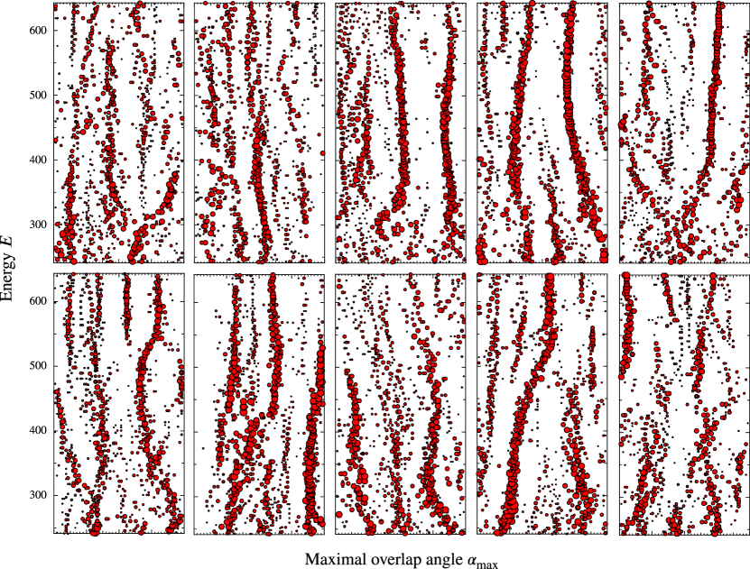
Figure 9: Montage of plots equivalent to Fig. 3, except than with ten other random realizations of the impurity positions. Each case shows branches of preferred orientations consisting of scarred eigenstates, although the strength of the branches and their stability with respect to eigenstate energy varies. In all plots the range of $\alpha_{\text{max}}$ is from $0$ to $2\pi/5$.

The RNG seed used for the realization discussed in the main article is 20141010. In the interest of full reproducibility, the version of itp2d used was 1.0.0-7-gd3c0454, with command line parameters:

itp2d --rngseed 20141010
   -F abschange(1e-3) -T absstdev(1e-3,5e-4)
   -l 11 -s 300 -e 0.01 -d 12 -t 6
   --noise impurities
   --impurity-distribution "uniform(2.0)"
   --impurity-type "gaussian(24, 0.1)"
   -n 4000 -N 5000
   -p "poweroscillator(5)"
   --maxsteps 50 --recover -D 2