The NuSTAR Extragalactic Surveys: The Number Counts of Active Galactic Nuclei and the Resolved Fraction of the Cosmic X-ray Background

Abstract

We present the 3 – 8 keV and 8 – 24 keV number counts of active galactic nuclei (AGN) identified in the NuSTAR extragalactic surveys. NuSTAR has now resolved 33 - 39% of the X-ray background in the 8 – 24 keV band, directly identifying AGN with obscuring columns up to $\sim 10^{25}$ cm^-2. In the softer 3 – 8 keV band the number counts are in general agreement with those measured by XMM-Newton and Chandra over the flux range $5\times 10^{-15}\mathbin{\lower 3.0pt\hbox{$\hbox to0.0pt{\raise 5.0pt\hbox{$\char 60\relax$}\hss}\mathchar 29208\relax$}}S{\rm(3-8keV)}/$erg s^-1 cm^-2$\mathbin{\lower 3.0pt\hbox{$\hbox to0.0pt{\raise 5.0pt\hbox{$\char 60\relax$}\hss}\mathchar 29208\relax$}}10^{-12}$ probed by NuSTAR. In the hard 8 – 24 keV band NuSTAR probes fluxes over the range $2\times 10^{-14}\mathbin{\lower 3.0pt\hbox{$\hbox to0.0pt{\raise 5.0pt\hbox{$\char 60\relax$}\hss}\mathchar 29208\relax$}}S{\rm(8-24~{}keV)}/$erg s^-1 cm^-2$\mathbin{\lower 3.0pt\hbox{$\hbox to0.0pt{\raise 5.0pt\hbox{$\char 60\relax$}\hss}\mathchar 29208\relax$}}10^{-12}$, a factor $\sim$100 fainter than previous measurements. The 8 – 24 keV number counts match predictions from AGN population-synthesis models, directly confirming the existence of a population of obscured and/or hard X-ray sources inferred from the shape of the integrated cosmic X-ray background. The measured NuSTAR counts lie significantly above simple extrapolation with a Euclidian slope to low flux of the Swift/BAT 15 – 55 keV number counts measured at higher fluxes ($S(15-55~{}{\rm keV})\mathbin{\lower 3.0pt\hbox{$\hbox to0.0pt{\raise 5.0pt\hbox{$\char 62\relax$}\hss}\mathchar 29208\relax$}}10^{-11}$ erg s^-1 cm^-2), reflecting the evolution of the AGN population between the Swift/BAT local ($z<0.1$) sample and NuSTAR’s $z\sim 1$ sample. CXB synthesis models, which account for AGN evolution, lie above the Swift/BAT measurements, suggesting that they do not fully capture the evolution of obscured AGN at low redshifts.

1. Introduction

A complete census of accreting supermassive black holes (SMBH) throughout cosmic time is necessary to quantify the efficiency of accretion, which is believed to drive the majority of SMBH growth (e.g. Soltan, 1982; Yu & Tremaine, 2002; Di Matteo et al., 2008; Merloni & Heinz, 2008). X-ray emission is nearly universal from the luminous Active Galactic Nuclei (AGN) that signal the most rapid SMBH growth phases, making surveys in the X-ray band particularly efficient at identifying accreting SMBH. Unlike optical and infrared light, X-rays are not diluted by host-galaxy emission, which is generally weak above $\sim$1 keV. X-rays are also penetrating, and hard ($\mathbin{\lower 3.0pt\hbox{$\hbox to0.0pt{\raise 5.0pt\hbox{$\char 62\relax$}\hss}\mathchar 29208\relax$}}$ 10 keV) X-rays are visible through columns up to $N_{\rm H}\sim 10^{25}$ cm^-2. For even higher columns AGN can be identified through scattered X-rays, although the emission becomes progressively weaker with increasing column.

Cosmic X-ray surveys with Chandra and XMM-Newton  have provided measurements of the demographics of the AGN population and its evolution in the 0.1 – 10 keV band out to large cosmic distances (see Brandt & Alexander, 2015, for a recent review). These surveys are sufficiently complete over a broad enough range of luminosity and redshift that many fundamental questions regarding AGN evolution can be addressed. In the deepest fields, $>80$% of the 2 – 10 keV Cosmic X-ray Background (CXB) has been resolved into individual objects (Hickox & Markevitch, 2006; Brandt & Alexander, 2015).

At X-ray energies above 10 keV the observational picture is far less complete. Coded-mask instruments such as INTEGRAL and Swift/BAT have probed the demographics of hard X-ray emitting AGN in the very local universe, to redshifts $z\mathbin{\lower 3.0pt\hbox{$\hbox to0.0pt{\raise 5.0pt\hbox{$\char 60\relax$}\hss}\mathchar 29208\relax$}}0.1$ (Tueller et al., 2008; Beckmann et al., 2009). The fraction of the CXB resolved by these instruments at its peak intensity (20 – 30 keV) is $\sim$1% (Krivonos et al., 2007; Ajello et al., 2012; Vasudevan, Mushotzky & Gandhi, 2013). Thus, until now, samples of AGN selected at $>10$ keV, which are inherently less biased by obscuration than those at lower energy, could not be used to probe AGN demographics, and in particular the evolution of highly obscured to Compton-thick ($N_{\rm H}\mathbin{\lower 3.0pt\hbox{$\hbox to0.0pt{\raise 5.0pt\hbox{$\char 62\relax$}\hss}\mathchar 29208\relax$}}\sigma_{\rm T}^{-1}\sim 10^{24}$ cm^-2) sources.

There is, therefore, strong motivation for extending sensitive X-ray surveys to high energy. Simple extrapolations of AGN populations detected by Chandra and XMM-Newton to higher energies based on average spectral properties fail to reproduce the shape and intensity of the CXB at 30 keV (e.g. Gilli, Comastri & Hasinger, 2007). This indicates either that spectral models based on the small samples of high-quality 0.1 - 100 keV measurements used in CXB synthesis models fail to capture the true spectral complexity of AGN, or that an additional highly obscured AGN population is present in the redshift range $0\mathbin{\lower 3.0pt\hbox{$\hbox to0.0pt{\raise 5.0pt\hbox{$\char 60\relax$}\hss}\mathchar 29208\relax$}}z\mathbin{\lower 3.0pt\hbox{$\hbox to0.0pt{\raise 5.0pt\hbox{$\char 60\relax$}\hss}\mathchar 29208\relax$}}2$. It is likely that both factors are important at some level. A higher fraction of reflected emission than typically assumed, which hardens the emission above 10 keV, appear to be present in moderately obscured, $23<\log(N_{\rm H}/$cm${}^{-2})<24$, AGN (Ricci et al., 2011). Even at moderate redshifts, reflection fractions are difficult to constrain with data restricted to $<10$ keV (e.g. Del Moro et al., 2014). In addition, it is difficult at low redshifts to properly measure high obscuring columns, which can lead to large errors in estimating intrinsic AGN luminosities (e.g. Lansbury et al., 2015). It is also challenging to identify Compton-thick objects in the range $0\mathbin{\lower 3.0pt\hbox{$\hbox to0.0pt{\raise 5.0pt\hbox{$\char 60\relax$}\hss}\mathchar 29208\relax$}}z\mathbin{\lower 3.0pt\hbox{$\hbox to0.0pt{\raise 5.0pt\hbox{$\char 60\relax$}\hss}\mathchar 29208\relax$}}2$ with the limited bandpass of Chandra and XMM-Newton (at $z\mathbin{\lower 3.0pt\hbox{$\hbox to0.0pt{\raise 5.0pt\hbox{$\char 62\relax$}\hss}\mathchar 29208\relax$}}$2 these missions sample rest frame energies above 20 keV). Thus both to characterize highly obscured AGN and constrain their evolution at $z\mathbin{\lower 3.0pt\hbox{$\hbox to0.0pt{\raise 5.0pt\hbox{$\char 60\relax$}\hss}\mathchar 29208\relax$}}2$ requires sensitive surveys at energies above 10 keV.

The Nuclear Spectroscopic Telescope Array (NuSTAR), the first focusing high-energy X-ray (3 - 79 keV) telescope on orbit (Harrison et al., 2013), has been executing a series of extragalactic surveys as part of its core program, with aim of measuring the demographics and properties of obscured AGN. Through contiguous surveys in fields with existing multi-wavelength data combined with dedicated spectroscopic followup of sources serendipitously identified in individual fields, the NuSTAR extragalactic surveys have improved the sensitivity limits in the hard, 8 – 24 keV band by two orders of magnitude relative to INTEGRAL or Swift/BAT, and have probed a wide range in redshift, out to $z\mathbin{\lower 3.0pt\hbox{$\hbox to0.0pt{\raise 5.0pt\hbox{$\char 62\relax$}\hss}\mathchar 29208\relax$}}2$.

In this paper we present the X-ray number counts (log $N$ - log $S$) of AGN, including the first sensitive measurements in the 8 – 24 keV band. We reach fluxes of $S$(8 – 24 keV)$\sim 3\times 10^{-14}$ erg s^-1 cm^-2, a factor of 100 deeper than previous measurements in this band. We compare the number counts to predictions from X-ray background synthesis models, and to extrapolations from Chandra and XMM-Newton surveys, and compare the intensity of resolved sources to that of the CXB. A companion paper (Aird et al., 2015a) presents direct constraints on the $>10$ keV AGN X-ray luminosity function. We adopt a flat cosmology with $\Omega_{\Lambda}=0.7$ and $h=0.7$, and quote 68.3% (i.e. 1$\sigma$ equivalent) errors unless otherwise noted.

2. Observations and Data Reduction

For the results in this paper we include all components of the NuSTAR extragalactic survey program that were completed and analyzed prior to March 2015. This includes coverage of well-studied contiguous fields as well as identification and followup of sources serendipitously detected in all NuSTAR fields. Figure 1 shows the area as a function of depth for the survey components included in this work. At the shallow end, NuSTAR surveyed 1.7 deg² of the Cosmic Evolution Survey field (COSMOS; Scoville et al. (2007)) to a depth of $S$(8 – 24 keV) = $1.3\times 10^{-13}$ erg s^-1 cm^-2. The catalog and results from this survey are presented in Civano et al. (2015) (hereafter C15). At the deep end, NuSTAR surveys have reached depths of $S$(8 – 24 keV) = $2.5\times 10^{-14}$ erg s^-1 cm^-2 in the Extended Chandra Deep Field South (ECDFS; Lehmer et al., 2005) over an area of 0.3 deg² and in the deep Chandra region of the Extended Groth Strip (Goulding et al., 2012; Nandra et al., 2015) over an area of 0.23 deg². The ECDFS source catalog is presented in Mullaney et al. (2015) (hereafter M15) and the EGS catalog will be presented in Aird et al. (in prep). The serendipitous survey adopts a similar approach used with the Chandra SEXSI survey (Harrison et al., 2003), where fields are searched for point sources not associated with the primary target, and subsequent spectroscopic followup with the Keck, Palomar 200-in, Magellan, and NTT telescopes provides redshifts and AGN classifications. Preliminary results from this survey were published in Alexander et al. (2013), and the 30-month catalog and results will be published in Lansbury et al. (in prep).

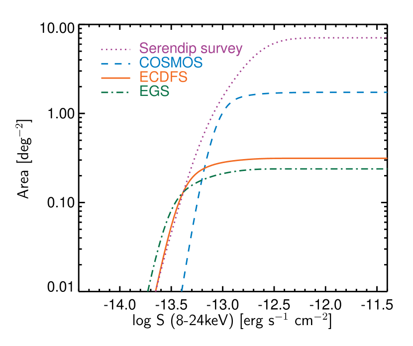
Figure 1.— Area as a function of depth in the observed 8 – 24 keV band for the NuSTAR extragalactic surveys included in this work.

The overall sample consists of 382 unique sources detected in the full (3 – 24 keV), soft (3 – 8 keV) or hard (8 – 24 keV) bands, of which 124 are detected in the hard band and 226 are detected in the soft band. Figure 2 shows the distribution of rest frame 10 – 40 keV luminosity versus redshift for the sources in our sample. Luminosities in this plot are derived from the 8 – 24 keV count rates (if detected in that band) assuming an unabsorbed X-ray spectrum with a photon index $\Gamma=1.8$ folded through the NuSTAR response. If the source is not detected in the 8 – 24 keV band we calculate luminosities using the 3 – 24 keV or (if not detected at 3 – 24 keV) the 3 – 8 keV count rates. The median redshift for the entire NuSTAR sample is $<z>=0.76$, with a median luminosity of $<\log(L_{\mathrm{10-40\;keV}}$/erg s${}^{-1})>=44.37$. For comparison we plot the distribution of AGN in the Swift/BAT 70-month catalog (Baumgartner et al., 2013). For reference, the dashed line in Figure 2 shows the location of the knee in the luminosity function as a function of redshift from the Chandra-based study of Aird et al. (2015b), extrapolated to the 10 – 40 keV band. Together, these surveys cover a broad range of luminosity and redshift.

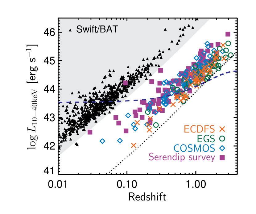
Figure 2.— Restframe 10 – 40 keV X-ray luminosity versus redshift for the objects included in this work compared to sources in the Swift/BAT 70-month all-sky survey catalog (black triangles). The dashed line shows the location of the knee in the luminosity function from Aird et al. (2015b) as a function of redshift. The shaded region indicates the region of sensitivity of Swift/BAT, and the dotted line indicates the threshold for the NuSTAR surveys.

2.1. Contiguous survey fields

We have adopted uniform source detection and flux extraction methodologies across the COSMOS, ECDFS and EGS survey fields. For the ECDFS and COSMOS fields we use the source lists and supporting data products (mosaic images, exposure maps and background maps in the 3 – 24 keV, 3 – 8 keV and 8 – 24 keV energy bands) from M15 and C15, respectively. We adopt exactly the same approach for the analysis of the EGS field (Aird et al., in prep.). We summarize the analysis approach here, and refer the reader to the relevant catalog papers for details.

For source detection we convolve both the mosaic images and background maps with a 20$\,{}^{\prime\prime}$-radius aperture at every pixel, and determine the probability, based on Poisson statistics, that the total image counts are produced by a spurious fluctuation of the background. We generate the background maps based on the NUSKYBGD code (see Wik et al., 2014, for details). We then identify groups of pixels in these false probability maps, using SExtractor, where the probability is less than a set threshold. Different thresholds are used in each field and in each energy band based on the expected number of spurious sources in simulations (see C15, M15 and Aird et al. in prep for specific values used for each field). We merge detections in multiple bands to produce the final catalogs, which include 61 sources (3 – 8 keV) and 32 sources (8 – 24 keV) in COSMOS, 33 sources (3 – 8 keV) and 19 sources (8 – 24 keV) in ECDFS, and 26 sources (3 – 8 keV) and 13 sources (8 – 24 keV) in EGS. The detection thresholds are chosen to ensure the catalogs are 99% reliable, Thus, we expect very few spurious sources (see M15, C15).

Source confusion must be corrected for since blended sources result in mis-estimation of source counts and fluxes. The NuSTAR PSF is relatively large compared to Chandra and XMM-Newton, and so source blending is particularly important to account for when comparing number counts from NuSTAR to these lower-energy, higher-resolution missions. The source de-blending procedure is described in detail in M15 and C15. To test the validity of the procedure we performed Monte Carlo simulations, where source fluxes were drawn from a published number counts distribution, counts maps were simulated, and sources were extracted and de-blended. We then verified that the resulting number counts distribution matches the input. The details of these simulations are provided in §4 of C15.

2.2. Serendipitous survey

The source-detection procedure for the serendipitous survey is the same as that outlined above, and described in detail in C15 and M15, although with a slightly different procedure for background determination. Many of the fields have bright central targets that contaminate a portion of the NuSTAR field-of-view. We thus take the original images and convolve them with an annular aperture of inner radius 30$\,{}^{\prime\prime}$ and outer radius 90$\,{}^{\prime\prime}$. We rescale the counts within this annulus to that of a 20$\,{}^{\prime\prime}$ radius region based on the ratio of the aperture areas and effective exposures. This procedure produces maps of the local background level at every pixel based on the observed images, and will thus include any contribution from the target object. We then use these background maps, along with the mosaic images, to generate false probability maps. From here the source detection follows that used in the contiguous fields, using a false probability threshold of $<10^{-6}$ across all bands. We exclude any detections within 90$\,{}^{\prime\prime}$ of the target position, and also any areas occupied by large, foreground galaxies or known sources that are associated with the target (but are not at the aimpoint). We also exclude areas where the effective exposure is $<20$% of the maximal (on-axis) exposure in a given field. Any NuSTAR fields at Galactic latitude $<20^{\circ}$ are also excluded from our sample. Full details of the serendipitous survey program will be provided in Lansbury et al. (in prep), which will also indicate those serendipitous fields used in this work. In total we include 106 serendipitous sources (3 – 8 keV) and 60 (8 – 24 keV).

3. Number count measurements

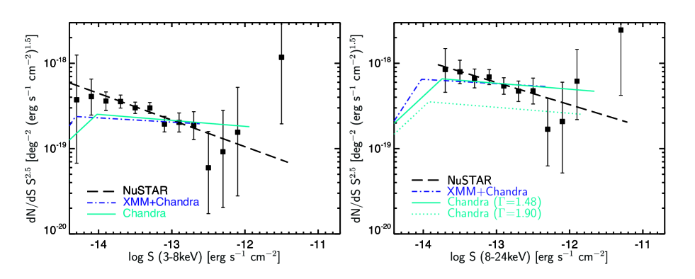
Figure 3.— Left panel: The differential number counts for the observed 3 – 8 keV band. The data points (black squares) show measurements from the combined NuSTAR survey fields, where error bars are 1$\sigma$ equivalent (i.e. 68.3% confidence level), and the black dashed line shows the best-fit power law. The solid line shows the best-fit to the number counts as measured by Chandra  (Georgakakis et al., 2008), and the dot-dashed line shows the best fit from a combined analysis of XMM-Newton and Chandra data (Mateos et al., 2008). Right panel: The differential logN-logS in the 8 – 24 keV band (black squares). The solid blue line and dot-dashed lines show the Chandra (4 – 7 keV) and XMM-Newton  measurements extrapolated to the 8 – 24 keV band using a photon power law index of $\Gamma=1.48$. The blue dotted line shows the Chandra measurements using a steeper ($\Gamma=1.9$) power law for the spectral extrapolation.

To determine the number counts (log $N$-log $S$), we adopt a Bayesian approach (see Georgakakis et al. 2008, Lehmer et al. 2012) that assigns a range of possible fluxes to a given source based on the Poisson distribution, which we then fold through the differential number counts distribution. We assume the differential number counts are described by a single power-law function;

$$\frac{dN}{dS}=K\left(\frac{S}{10^{-13}~{}\rm{erg~{}s^{-1}~{}cm^{-2}}}\right)^{\beta}$$ (1)

where $K$ is the normalization at $S=10^{-13}$ erg s^-1 cm^-2 and $\beta$ is the slope. Folding the Poisson likelihood for each individual source through the differential number counts given by Equation 1 accounts for the Eddington bias, allowing for the fact that a detection is more likely to be due to a positive fluctuation from a source of lower flux than vice-versa. We limit the range of possible source fluxes to a factor 3 below the nominal flux limit to prevent the probability distribution from diverging at the faintest fluxes as a result of our assumed power-law function.

We optimize the values of the parameters describing the power-law model for the differential number counts by performing an un-binned maximum likelihood fit for all sources detected in a given band (see Georgakakis et al. 2008). We also estimate differential source number counts in a number of fixed-width bins in flux using the $N_{\mathrm{obs}}/N_{\mathrm{mdl}}$ method of Miyaji, Hasinger & Schmidt (2001), as expanded on in Aird et al. (2010), to account for flux probability distributions. The binned estimate of the differential source number counts is then given by

$$\left[\frac{dN}{dS}\right]_{\mathrm{bin}}=\left[\frac{dN}{dS}\right]_{\mathrm{mdl}}\frac{N_{\mathrm{obs}}}{N_{\mathrm{mdl}}}$$ (2)

where $\left[\frac{dN}{dS}\right]_{\mathrm{mdl}}$ corresponds to the power-law model for the differential number counts evaluated at the center of the bin, $N_{\mathrm{mdl}}$ is the predicted number of sources in a bin (found by folding the model through the sensitivity curve) and $N_{\mathrm{obs}}$ is the effective observed number of sources, allowing for the distribution of possible fluxes (thus a single source can make a partial contribution to multiple bins). We estimate errors based on Poisson uncertainties in $N_{\mathrm{obs}}$ as given by Gehrels (1986).

Figure 3 (left) shows the resulting differential source number densities based on the NuSTAR samples from the four survey components combined, in the 3–8 keV band. We also compare the NuSTAR measurements to the best-fit broken power-law functions determined from Chandra surveys by Georgakakis et al. (2008) and a joint analysis of XMM-Newton and Chandra surveys by Mateos et al. (2008). We convert the Chandra (4 – 7 keV) and XMM-Newton (2 – 10 keV) number counts to match the 3–8 keV NuSTAR band assuming a $\Gamma=1.8$ power-law X-ray spectrum. Because the bands are largely overlapping, the choice of photon spectral index does not significantly affect the results. To ease comparison between the different results we have scaled $dN/dS$ by the Euclidean slope, $S^{-2.5}$. The NuSTAR measurements constrain the slope well over the range $-14<\log(S/$erg s^-1 cm^-2$)<-12.5$. The best fit values for the power law parameters in this band are: log $K=13.84\pm 0.04$, $\beta=-2.81\pm 0.08$.

The NuSTAR results generally agree with Chandra and XMM-Newton, although the slope of the number counts with flux is somewhat steeper. Below $S\sim 10^{-14}$ erg s^-1 cm^-2 the NuSTAR measurements are poorly constrained, so that the location of the break in the number counts seen by Chandra and XMM-Newton cannot be independently confirmed. The difference in slope of the number counts with flux between NuSTAR and the soft X-ray telescopes is due the different instrument responses and the corresponding uncertainties in converting count rates to fluxes based on simple spectral models. To verify this we folded the population synthesis model of Aird et al. (2015b) through the NuSTAR response function to predict the observed count-rate distribution. We convert the count rates to fluxes, applying our standard count rate to flux conversion factor. We repeated this exercise adopting the Chandra response function, applying the count rate to flux conversion factor from Georgakakis et al. (2008). For moderately to heavily absorbed sources ($N_{\mathrm{H}}\sim 10^{23}$ cm^-2), the expected count rates are more strongly suppressed using the Chandra response (as the NuSTAR instrument response is more strongly weighted to higher energies). The intrinsic fluxes are therefore underestimated for such sources with Chandra when a single conversion factor is assumed. We have verified that this effect leads to an slope difference in the expected log $N$ – log $S$ at $f_{\mathrm{3-8keV}}\sim 10^{-14}-10^{-13}$ erg s^-1cm^-2 that matches the discrepancy seen between the NuSTAR measurements and the Chandra and XMM-Newton measurements shown in Figure 3 (left). Figure 4 (left) shows the integral number counts in the 3 – 8 keV band.

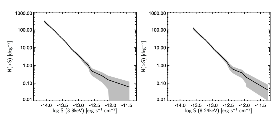
Figure 4.— Integral number counts for the 3 – 8 keV (left) and 8 – 24 (right) observed bands. The grey shaded region shows the 68.3% confidence region on the integrated number counts based on the Poisson error in the number of sources weighted by the survey area as a function of flux. The blue line on the left plot shows a comparison to Chandra counts extrapolated from 4 – 7 keV.

Figure 3 (right) shows the differential source number counts in the 8 – 24 keV band, along with the best fit power law, parametrized by log $K=14.3\pm 0.04$, and $\beta=-2.76\pm 0.10$. We also plot extrapolations of the Mateos et al. (2008) Chandra+ XMM-Newton counts and the Georgakakis et al. (2008) Chandra counts to the harder, largely non-overlapping 8 – 24 keV band (dotted and solid lines in Figure 3). The dotted line shows the extrapolation assuming $\Gamma=1.8$, which is typical of unabsorbed AGNs, and systematically underpredicts the NuSTAR measurements. Using a maximum likelihood analysis, we find that a spectral photon index of $\Gamma=1.48$ (solid line) provides the best match between the extrapolation of the Georgakakis et al. (2008) model and the NuSTAR data, indicating that a substantial population of absorbed and/or hard-spectrum sources is required to reproduce the NuSTAR measurements.

4. Comparison with the Swift/BAT Local AGN Sample

In combination, NuSTAR and Swift/BAT sample the hard X-ray AGN population over a wide range in flux and redshift. Swift/BAT has measured the number counts at fluxes $S\mathbin{\lower 3.0pt\hbox{$\hbox to0.0pt{\raise 5.0pt\hbox{$\char 62\relax$}\hss}\mathchar 29208\relax$}}3\times 10^{-12}$ erg s^-1 cm^-2 in the 15 – 55 keV band for the local ($z\mathbin{\lower 3.0pt\hbox{$\hbox to0.0pt{\raise 5.0pt\hbox{$\char 60\relax$}\hss}\mathchar 29208\relax$}}0.1$) AGN sample (Ajello et al., 2012). Although there is a gap in the flux range probed by BAT and the $S\mathbin{\lower 3.0pt\hbox{$\hbox to0.0pt{\raise 5.0pt\hbox{$\char 60\relax$}\hss}\mathchar 29208\relax$}}3\times 10^{-13}$ erg s^-1 cm^-2 population probed by NuSTAR, extrapolating the BAT differential number counts to fainter fluxes indicates whether there is any evolution between the low-redshift BAT AGN population and the higher-redshift NuSTAR sources.

Figure 5 shows the NuSTAR 8 – 24 keV number counts together with the BAT measurements from Ajello et al. (2012), which are well described by a single power-law $dN/dS$ with slope $\beta\approx 2.5$ (bold dashed line). We have converted the BAT 15 - 55 keV fluxes to the 8 – 24 keV band assuming a photon index of $\Gamma=1.7$, the value that provides the best fit to the average BAT AGN spectral model from Burlon et al. (2011). The hatched region indicates the measurement uncertainties from Ajello et al. (2012), showing that the formal error is small, about the width of the dashed line. It is clear that the extrapolation of the BAT counts to lower fluxes where the counts are well-constrained by NuSTAR ($f\sim 10^{-13.5}$erg s^-1 cm^-2 significantly under-predicts the NuSTAR measurements. This disagreement is not surprising, since there is strong evolution in the AGN population between the local ($z\sim 0.1$) BAT sample and the higher-redshifts probed by NuSTAR.

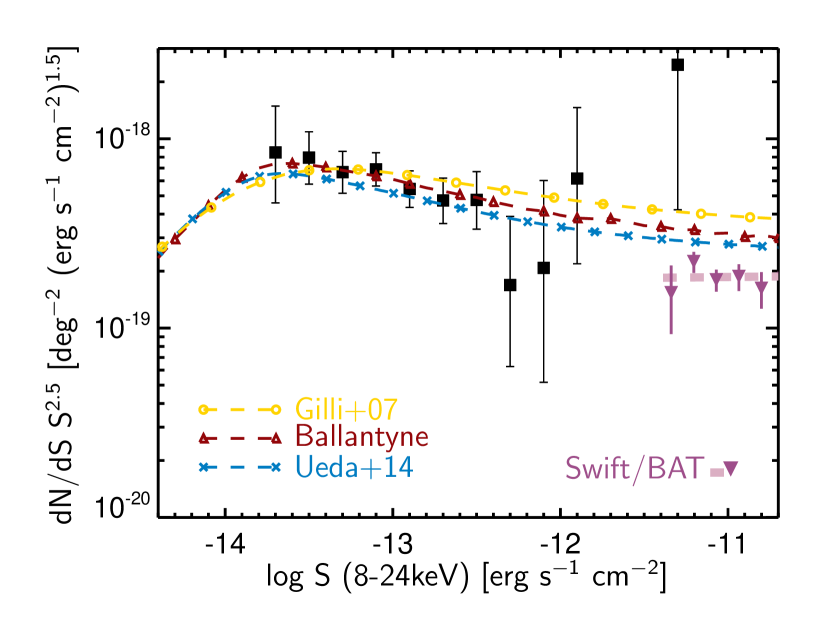
Figure 5.— The NuSTAR 8 – 24 keV number counts compared to Swift/BAT (bold dashed line) (Ajello et al. 2012). The hatched region indicates the uncertainty in the overall fit from Ajello et al. (2012). We convert the BAT 15-55 keV band to the 8 – 24 keV band using a power law with photon index $\Gamma=1.7$ (the best-fit to the average BAT AGN spectrum in the 15 – 55 keV band). The dashed line with triangles shows predictions from the CXB synthesis model of Ballantyne 2011 updated to use the Ueda 2014 luminosity function. The dashed line with crosses shows the population synthesis model from Ueda et al. (2014). The dashed line with circles shows predictions from the CXB model from Gilli, Comastri & Hasinger (2007). The plotted errors are 1-$\sigma$.

5. Comparison with X-ray Background Synthesis Models

The existence of a population of obscured and Compton thick objects beyond those directly resolved below 10 keV has long been postulated by CXB synthesis models. These models reproduce the hard spectrum of the CXB using measured AGN X-ray luminosity functions (XLFs), which are well constrained (except in the very local universe) only below 10 keV, together with models for the broadband ($\sim$1 – 1000 keV) AGN spectra and estimates of the Compton-thick AGN fraction and its evolution (e.g. Gilli, Comastri & Hasinger (2007), Treister, Urry & Virani (2009), Ueda et al. (2014)). The XLF measurements, assumptions about AGN spectral evolution, and Compton-thick fractions differ significantly among models.

Figure 5 compares the NuSTAR counts to three different CXB synthesis models: the model from Gilli, Comastri & Hasinger (2007) (dashed line with circles), the model of Ueda et al. (2014), and an an updated version of the Ballantyne (2011) model. The details of the Gilli, Comastri & Hasinger (2007) and Ueda et al. (2014) models are documented in the relevant publications. The updated Ballantyne model differs from Ballantyne (2011) in that it uses the new Ueda et al. (2014) luminosity function, a better spectral model from Ballantyne (2014), the Burlon et al. (2011) N_H distribution, and the redshift evolution and obscured fraction from Ueda et al. (2014). Other aspects, including the normalization of the Compton-thick fraction are the same as in Ballantyne (2011). We include this model because it fits the CXB spectrum even after including the effects of blazers.

All three models are in good agreement with the measured NuSTAR counts. However, all of the models lie significantly above the Swift/BAT measurements at $S\mathbin{\lower 3.0pt\hbox{$\hbox to0.0pt{\raise 5.0pt\hbox{$\char 62\relax$}\hss}\mathchar 29208\relax$}}10^{-11.5}$erg s^-1 cm^-2. The discrepancy between the BAT measurements and the models cannot be accounted for by uncertainties in the spectral shape; a spectral index of $\Gamma=2.1$ when converting to the 8 - 24 keV band is required to make the Swift/BAT 15 – 55 keV measurements agree with the model predictions. This is significantly softer than the average measured spectral shape, even for unobscured AGN, and can thus be ruled out. Therefore, this discrepancy appears to be due to evolution in the hard XLF, absorption distribution, or spectral properties of AGN between the very local Swift/BAT sample and the more distant ($z\sim 0.5-1$) NuSTAR sample that is not fully accounted for in these population synthesis models (see also Aird et al. 2015b).

6. Summary and Conclusions

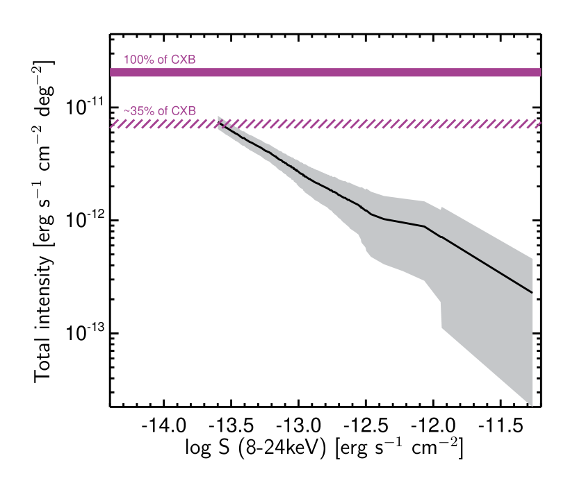
Figure 6.— Total intensity as a function of 8 - 24 keV flux of the resolved sources in the sample included in this work. The horizontal lines indicate 35% (hatched line) and 100% (solid line) of the cosmic X-ray background (CXB). The width of the lines indicates the range of normalizations determined by different instruments (see Table 1 for references). At the faint end of the surveys included here NuSTAR is resolving $\sim$35% of the CXB.

We have presented measurements of the number counts of AGN with NuSTAR  in two bands, from 3 – 8 keV and 8 – 24 keV. The data span a broad range in flux, with good constraints covering $10^{-14}\mathbin{\lower 3.0pt\hbox{$\hbox to0.0pt{\raise 5.0pt\hbox{$\char 60\relax$}\hss}\mathchar 29208\relax$}}$ S (8 - 24 keV; erg s^-1 cm^-2) $\mathbin{\lower 3.0pt\hbox{$\hbox to0.0pt{\raise 5.0pt\hbox{$\char 60\relax$}\hss}\mathchar 29208\relax$}}10^{-13}$. The 3 – 8 keV differential source number densities are in agreement with measurements from Chandra and XMM-Newton, although the slope measured by NuSTAR is somewhat steeper. The slope difference results from the fact that the NuSTAR effective area curve is weighted to significantly higher energies compared to XMM-Newton and Chandra, which results in the observed discrepancy when using a simple counts to flux conversion factor.

Table 1 X-ray Background Measurements

Instrument	$I_{CXB}$ (20 - 50 keV)	$I_{CXB}$ (8 - 24 keV)	% resolved by NuSTAR
HEAO-1 A2 + A4	$6.06\pm 0.06$	$6.33\pm 0.07$	39
HEAO-1 A2	$5.60\pm 0.30$	$6.27\pm 0.33$	39
BeppoSAX	$5.89\pm 0.19$	$6.48\pm 0.21$	38
INTEGRAL	$\sim 6.66$	$7.33$	33
BAT	$6.50\pm 0.15$	$7.16\pm 0.17$	34

Note. — CXB intensity ($I_{CXB}$) is given in units of $10^{-8}$ergs cm^-2 s^-1 sr^-1. Intensities in the 20 – 50 keV band are taken from Gruber et al. (1999) for HEAO-1 A2 + A4, Marshall et al. (1980) for HEAO-1 A2, Frontera et al. (2007) for BeppoSAX, Churazov et al. (2007) for INTEGRAL, and Ajello et al. (2008) for BAT.

In the 8 – 24 keV band we present the first direct measurement of the AGN number counts that includes data above $\sim$10 keV and reaches down to flux levels $\sim 3\times 10^{-14}$ erg s^-1 cm^-2. In order to match the NuSTAR number counts, the flux measurements from Chandra and XMM-Newton must be extrapolated to higher energy using a spectrum with photon index $\Gamma=1.48$. This photon index is significantly harder than the $\Gamma=1.7-1.9$ that characterizes the unobscured AGN population, and is also significantly harder than the average spectral index that characterizes the Swift/BAT AGN sample.

The NuSTAR number counts are in good agreement with predictions from population synthesis models that explain the hard spectrum of the CXB using different assumptions about obscuration, the Compton thick sample, and the spectra shape of AGN in the hard X-ray band (see Figure 5). This directly confirms the existence of a population of AGN with harder spectra than those typically measured below 10 keV. The spectral hardness could be due either to increased reflection or near Compton-thick absorption. The updated Ballantyne model, for example, uses an AGN spectral model with a strong Compton reflection component with a relative normalization component of $R=1.7$. Our measurements of the rest-frame 10 – 40 keV XLF Aird et al. (2015a) also indicate that a significant population of AGN with hard X-ray spectra is required to reconcile our NuSTAR data with prior, lower energy XLF measurements. To what extent this results from obscuration versus higher levels of reflection will be determined by spectral analysis of NuSTAR sources in the survey fields (Del Moro et al. in prep, Zappacosta et al. in prep), and from spectral modeling of high quality data from local AGN samples (Baloković et al. in prep).

The NuSTAR 8 – 24 keV number counts lie significantly above a direct extrapolation with flux of the number counts at brighter fluxes, sampled by the Swift/BAT survey in the 15 – 55 keV band (Figure 5). This discrepancy is not surprising given the known evolution of the AGN population between the low redshift Swift/BAT AGN and the higher redshift NuSTAR sample It is interesting that the BAT data are in tension with CXB synthesis models (see Figure 5), which are in good agreement with the NuSTAR measurements. The most natural explanation for the difference is an evolution in the hard XLF, absorption distribution, or spectral properties of AGN between the very local objects seen by BAT and the more distant ($z\sim 0.5-1$) NuSTAR sample that is not accounted for in the current population synthesis models.

Table 1 provides CXB fluxes measured by hard X-ray instruments in the 20 - 50 keV and 8 – 24 keV bands. To convert the intensities to the 8 – 24 keV band for those instruments that do not cover this energy range (BeppoSAX, INTEGRAL, Swift/BAT) we used Equation 5 of Ajello et al. (2008), which parametrizes the CXB spectrum between 2 keV and 2 MeV based on a fit to available data. The NuSTAR extragalactic surveys have reached depths of $S$(8 – 24 keV)$\approx 3\times 10^{-14}$ erg s^-1 cm^-2. Comparing to the total integrated flux of the CXB as measured by collimated and coded aperture instruments shown in Table 1, this corresponds to a resolved fraction of 33 - 40% in the 8 – 24 keV band (Figure 6), with an additional statistical uncertainty of 5%. Even for the highest measured CXB flux from Churazov et al. (2007) NuSTAR still resovles 33%, which is a significant advance compared to the 1 - 2% resolved to-date by coded mask instruments above 10 keV (Vasudevan, Mushotzky & Gandhi, 2013; Krivonos et al., 2007).

The resolved fraction of the CXB we measure is in good agreement with pre-launch predictions based on CXB synthesis models Ballantyne et al. (2011). At the current depth the NuSTAR surveys do not probe the break in the number counts distribution, expected, based on extrapolations from Chandra and XMM-Newton, to occur at $S$(8 – 24 keV)$\sim$10^-14 erg s^-1 cm^-2. Reaching these depths will be challenging, as the deep fields are currently background dominated, such that sensitivity improves only as the square root of observing time. However, additional exposure in the ECDFS is planned, along with expansion of the deep surveys to cover the CANDELS/UDS field (Grogin et al., 2011), and continuation of the serendipitous survey, which will better constrain the slope of the number counts distribution above the break and improve spectral constraints on the resolved AGN population.

References

- Aird et al. (2015a) Aird, J., Alexander, D., Ballantyne, D., Civano, F., & Mullaney, J., 2015a, ApJ, 815, 66
- Aird et al. (2015b) Aird, J., Coil, A. L., Georgakakis, A., Nandra, K., Barro, G., & Pérez-González, P. G., 2015b, MNRAS, 451, 1892
- Aird et al. (2010) Aird, J., et al., 2010, MNRAS, 401, 2531
- Ajello et al. (2012) Ajello, M., Alexander, D. M., Greiner, J., Madejski, G. M., Gehrels, N., & Burlon, D., 2012, ApJ, 749, 21
- Ajello et al. (2008) Ajello, M., et al., 2008, ApJ, 689, 666
- Alexander et al. (2013) Alexander, D. M., et al., 2013, ApJ, 773, 125
- Ballantyne (2014) Ballantyne, D. R., 2014, MNRAS, 437, 2845
- Ballantyne et al. (2011) Ballantyne, D. R., Draper, A. R., Madsen, K. K., Rigby, J. R., & Treister, E., 2011, ApJ, 736, 56
- Baumgartner et al. (2013) Baumgartner, W. H., Tueller, J., Markwardt, C. B., Skinner, G. K., Barthelmy, S., Mushotzky, R. F., Evans, P. A., & Gehrels, N., 2013, ApJS, 207, 19
- Beckmann et al. (2009) Beckmann, V., et al., 2009, A&A, 505, 417
- Brandt & Alexander (2015) Brandt, W. N., & Alexander, D. M., 2015, A&A Rev., 23, 1
- Burlon et al. (2011) Burlon, D., Ajello, M., Greiner, J., Comastri, A., Merloni, A., & Gehrels, N., 2011, ApJ, 728, 58
- Churazov et al. (2007) Churazov, E., et al., 2007, A&A, 467, 529
- Civano et al. (2015) Civano, F., et al., 2015, ApJ, 808, 185
- Del Moro et al. (2014) Del Moro, A., et al., 2014, ApJ, 786, 16
- Di Matteo et al. (2008) Di Matteo, T., Colberg, J., Springel, V., Hernquist, L., & Sijacki, D., 2008, ApJ, 676, 33
- Frontera et al. (2007) Frontera, F., et al., 2007, ApJ, 666, 86
- Gehrels (1986) Gehrels, N., 1986, ApJ, 303, 336
- Georgakakis et al. (2008) Georgakakis, A., Nandra, K., Laird, E. S., Aird, J., & Trichas, M., 2008, MNRAS, 388, 1205
- Gilli, Comastri & Hasinger (2007) Gilli, R., Comastri, A., & Hasinger, G., 2007, A&A, 463, 79
- Goulding et al. (2012) Goulding, A. D., et al., 2012, ApJS, 202, 6
- Gruber et al. (1999) Gruber, D. E., et al., 1999, ApJ, 520, 124
- Grogin et al. (2011) Grogin, N. A., et al., 2011, ApJS, 197, 35
- Harrison et al. (2013) Harrison, F. A., et al., 2013, ApJ, 770, 103
- Harrison et al. (2003) Harrison, F. A., Eckart, M. E., Mao, P. H., Helfand, D. J., & Stern, D., 2003, ApJ, 596, 944
- Hickox & Markevitch (2006) Hickox, R. C., & Markevitch, M., 2006, ApJ, 645, 95
- Krivonos et al. (2007) Krivonos, R., Revnivtsev, M., Lutovinov, A., Sazonov, S., Churazov, E., & Sunyaev, R., 2007, A&A, 475, 775
- Lansbury et al. (2015) Lansbury, G. B., et al., 2015, ArXiv e-prints
- Lehmer et al. (2005) Lehmer, B. D., et al., 2005, ApJS, 161, 21
- Lumb et al. (2002) Lumb, D. H., et al., 2002, A&A, 389, 93
- Marshall et al. (1980) Marshall, F., et al., 1970, ApJ, 235, 4
- Mateos et al. (2008) Mateos, S., et al., 2008, AAP, 492, 51
- Merloni & Heinz (2008) Merloni, A., & Heinz, S., 2008, MNRAS, 388, 1011
- Miyaji, Hasinger & Schmidt (2001) Miyaji, T., Hasinger, G., & Schmidt, M., 2001, A&A, 369, 49
- Mullaney et al. (2015) Mullaney, J. R., et al., 2015, ApJ, 808, 184
- Nandra et al. (2015) Nandra, K., et al., 2015, ArXiv e-prints
- Ricci et al. (2011) Ricci, C., Walter, R., Courvoisier, T. J.-L., & Paltani, S., 2011, A&A, 532, A102
- Scoville et al. (2007) Scoville, N., et al., 2007, ApJS, 172, 1
- Soltan (1982) Soltan, A., 1982, MNRAS, 200, 115
- Treister, Urry & Virani (2009) Treister, E., Urry, C. M., & Virani, S., 2009, ApJ, 696, 110
- Tueller et al. (2008) Tueller, J., Mushotzky, R. F., Barthelmy, S., Cannizzo, J. K., Gehrels, N., Markwardt, C. B., Skinner, G. K., & Winter, L. M., 2008, ApJ, 681, 113
- Ueda et al. (2014) Ueda, Y., Akiyama, M., Hasinger, G., Miyaji, T., & Watson, M. G., 2014, ApJ, 786, 104
- Vasudevan, Mushotzky & Gandhi (2013) Vasudevan, R. V., Mushotzky, R. F., & Gandhi, P., 2013, ApJ, 770, L37
- Wik et al. (2014) Wik, D. R., et al., 2014, ApJ, 792, 48
- Yu & Tremaine (2002) Yu, Q., & Tremaine, S., 2002, MNRAS, 335, 965