On the Control of Self-Balancing Unicycles

Abstract

This paper discusses the problem of designing a self-balancing unicycle where pedals are used for both power generation and speed control. After developing the principal physical aspects (in the longitudinal dimension), we describe an abstract model in the form of a collection of hybrid automata, together with design requirements to be met by an ideal controller. We discuss simplifications and assumptions that make this model amenable to verification and validation tools such as SpaceEx. To enable experimentation with different prototypical controllers and user behaviours in concrete scenarios, we also develop a simple simulation framework using digital time.

1 Introduction

During the last decade, self-balancing devices for individual (short-distance) travel have gained popularity. The most prominent example is the Segway, a two wheeler with a handrail for the user to hold on to, but there are also devices that require the user to stand freely on a single wheel, such as the Solowheel. In both designs the tilting of the foot rest is continuously taken as sensor input, and interpreted as the intention to accelarate or slow down. Accelaration is thus the result of leaning forwards (or pushing the handrail, or tilting the feet downwards), and conversely for deacceleration.

For classical pedal-powered unicylces the task of speed control and of balancing is entirely left to the rider. In this work, we analyze self-balancing unicycles which structurally resemble a normal unicycle, but are characterised by the following three properties:

1. The unicycle needs to be balanced both longitudinally and laterally.

2. As with a normal cycle, the rider influences the speed by pedaling, not by leaning forwards or backwards.

3. The seat post is to be kept stably upright, thus perpendicular to the ground horizon.

In particular, this implies that the rider does effectively not lean forwards or backwards independent of the device’s wheel rotation since he has a fixed seat position.

We are looking for a controller that enables the above features. Our design is meant to echo the concept of a pedelec, a pedal-assisted electric two-wheel bicycle. A pedelec supports the rider by an electric motor, which emits additional power to one of the rotating wheels proportional to the measured pedalling activity. The electric power is drawn from an on-board battery. Pedelecs are rapidly gaining popularity in many countries, especially across central Europe.

We assume a unicylce construction where the pedals are mounted to a generator, providing electric power to the system and at the same time indicating the current intended riding speed to the controller. The pedals are thus not connected to the wheel. This is because otherwise the needed corrective torques will have to interfere with the pedalling feet, making it presumably very inconvenient to ride smoothly. Instead, a hub motor is mounted between the wheel and the rods the saddle is mounted on. This motor can therefore enact a torque between the wheel and the saddle, and thus the rider.

This paper develops the principal physical aspects focussing on the longitudinal dimension, thus assuming that it is the rider’s responsibility not to fall over laterally (just as when riding an ordinary bicycle). We represent the system as a collection of hybrid automata and discuss design requirements to be met by an ideal controller. We then turn our attention to simplifying assumptions so as to make this model amenable to verification and validation tools for affine dynamics. In this we mainly target SpaceEx [5], one of the most advanced verification environments in this context. We also discuss briefly how prototypical controller instances can be experimented with on the abstract model, making use of a simple simulation framework using digital time.

To the best of our knowledge, the problem of designing a pedal-assisted electric unicycle is in itself novel, yet it is very intriguing. Solving it will mean the conception of the lightest pedelec ever built, and this might come with commercialisation chances for commuter traffic in urban areas, for instance. Related work covers the classical inverted pendulum [4], as well as Segway-style designs [7].

The paper is organized as follows. In Section 2, we discuss the physical aspects of such a unicycle. Section 3 develops the hybrid automata model, and Section 4 discusses controller designs for it. In Section 5, we lay out our verification efforts, and Section 6 briefly reviews a simulation framework for our model. Finally, in Section 7, we conclude.

2 Aspects of the Model

2.1 A Unicycle

Basic Setup.

We begin by discussing the behaviour of a pure unicycle. Our model of a unicycle is sketched in Figure 1. At the bottom, there is a large wheel $W$. In its centre, a long rod is affixed which has the saddle mounted on its top. The rider sits on the saddle. We assume that rod, saddle and rider do not move relative to each other and call the resulting object saddle ($S$).

We consider only two external forces influencing this system:

1. gravity, pulling down on $S$, and

2. a torque $\tau_{W,\mathit{mot}}$ applied between $W$ and $S$, caused by a motor mounted there (where a positive torque rotates $W$ counter-clockwise and $S$ clockwise).

To simplify the model, we assume the following:

1. There are no lateral forces, so the forces we consider live in a two-dimensional vector space.

2. The friction between $W$ and the ground is high enough for the wheel to never slide.

Then, the model can be described by the parameters specified in Section 2.1. A state of the model is represented by the variables in Section 2.1.

o 0.9X[1]X[5]    parameter	description
$r_{W}$	the radius of wheel $W$
$r_{\mathit{com}}$	the distance from the bottom of $S$ to its center of mass
$r_{S}$	the distance from the bottom of $S$ to the top
$m_{W,\mathit{real}}$	the actual mass of $W$
$m_{S}$	the mass of $S$, including the driver’s mass
$I_{S}$	the moment of inertia of $S$
$I_{W}$	the moment of inertia of $W$
$\xi$	constant with $\xi\in[0.5,1]$ describing the distribution of the mass in the wheel, see Section A.1
$\tau_{\mathit{max}}$	the maximum torque the motor can enact in any direction

Table 1: Parameters of the System

o 0.9X[1.5]X[5]    state variable	description
$x_{W}$	the $x$-coordinate of the wheel
$v_{W}$	the horizontal speed of the wheel
$\theta$	the angle of the rod, relative to its upright position
$\omega_{S}$	the angular speed of the rod

Table 2: State of the System

Equations of Motion.

We now briefly summarize the equations of motion. Their full derivation can be found in Appendix A.

The torque $\tau_{W,\mathit{mot}}$ rotates the wheel $W$ counter-clockwise, which corresponds to a force $F_{W,\mathit{mot}}$ that pulls $W$ to the right with

$$F_{W,\mathit{mot}}=-\frac{-\tau_{W,\mathit{mot}}}{r_{W}}.$$

Gravity pulls down on $S$. If it is not in the upright position, this causes a counter-clockwise $\tau_{S,g}$ with

$$\tau_{S,g}=m_{s}\cdot g\cdot\sin\theta\cdot r_{\mathit{com}}$$

and a force $F_{W,g}$ that pushes $W$ to the right with

$$F_{W,g}=m_{s}\cdot g\cdot\cos\theta\cdot\sin\theta.$$

We now have collected all longitudinal forces that act on $W$, we call their sum $F_{W}$:

$$F_{W}=F_{W,\mathit{mot}}+F_{W,g}$$

This force acts on $W$, which is affixed to $S$. To analyse the impact of this force on the system, we split it into two parts $F_{W,1}+F_{W,2}=F_{W}$, where $F_{W,1}$ and $F_{W,2}$ can be seen as acting on $S$ in isolation and the wheel $W$ in isolation, respectively:

$$m_{W} =m_{W,\mathit{real}}+\xi\cdot m_{W,\mathit{real}}$$ (8)

$$\beta =\frac{m_{S}}{m_{W}}\cdot\left(1+3\cos^{2}\theta\right)$$ (18)

$$F_{W,1} =F_{W}\cdot\frac{\beta}{1+\beta}$$ (19)

$$F_{W,2} =F_{W}\cdot\frac{1}{1+\beta}$$ (20)

While $F_{W,2}$ can now be seen as the only force affecting the longitudinal movement of the unicycle (or more specifically its wheel), $F_{W,1}$ has a more complicated influence: It causes a counter-clockwise torque $\tau_{S,W}$ on $S$ with strength

$$\tau_{S,W}=F_{W,1}\cdot r_{\mathit{com}}\cdot\cos\theta.$$

We now know all torques acting on $S$:

$$\tau_{S}=-\tau_{W,\mathit{mot}}+\tau_{S,g}+\tau_{S,W}.$$

Having considered all forces and torques, we can now give differential equations for the $x$-position, speed, angle and angular velocity of the unicycle:

$$\dot{x_{W}} =v_{W}$$ (23)

$$\dot{v_{W}} =\frac{F_{W,2}}{m_{W}}$$ (24)

$$\dot{\theta} =\omega$$ (25)

$$\dot{\omega} =\frac{\tau_{S}}{I_{S}}$$ (26)

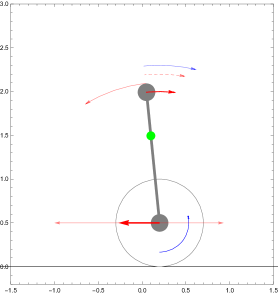
Figure 1: A Simplified Unicycle With Forces The blue arrows both represent $\tau_{W,\mathit{mot}}$. The thin red arrows on the wheel represent $F_{W,\mathit{mot}}$ (to the left) and $F_{W,g}$ (to the right), while the thick one is $F_{W}$. The red dashed torque on the rod is $\tau_{S,W}$, the thin, solid one shows $\tau_{S,g}$. Here, too, the thick arrow represents the sum, $\tau_{S}$.

Figure 1 displays an exemplary state of the unicycle where all linear forces and torques are indicated.

2.2 Surrounding Components

In addition to the unicycle, we need to add three additional components to the model: user, controller and motor.

Since we are considering a device where the pedals generate electric power and indicate the intended speed, the user has no other influence on the actual unicycle. Therefore, we model the user as a black-box component that sets a variable $\mathit{userIntent}$, indicating the target speed.

The controller may use the unicycle’s state variables and $\mathit{userIntent}$ to compute the torque the motor should enact, and sets this as $\mathit{motorTorque}$. We only consider controllers where the development of $\mathit{motorTorque}$ over time is continuous and differentiable.

Finally, the motor is a model of the physical constraints of the motor’s capabilities. It uses $\mathit{motorTorque}$ to set the actual force $\tau_{W,\mathit{mot}}$ applied between saddle and wheel. In our model, this is simply $\mathit{motorTorque}$ capped to the maximal strength of the motor, which we denote by $\tau_{\mathit{max}}$.

3 A Hybrid Automaton Model

In the following, we consider a fixed unicycle and therefore consider the parameters specified in Section 2.1 and $\tau_{\mathit{max}}$ to be constants. We use the hybrid (input/output) automata (HIOA) formalism [3] due to its conciseness and adequacy. We assume familiarity with this notation, which we shall use in its intuitive pictorial form below.

Unicycle.

The unicycle behaviour is represented as the HIOA $\mathcal{O}=(A_{\mathcal{O}},C_{\mathcal{O}},O_{\mathcal{O}})$ over variables $X_{\mathcal{O}}=\left\{\tau_{W,\mathit{mot}},x_{W},v_{W},\theta,\omega\right\}$ with hybrid automaton [2] $A_{\mathcal{O}}$ as depicted in 2(a), controlled variables $C_{\mathcal{O}}=\left\{x_{W},v_{W},\theta,\omega\right\}$, output variables $O_{\mathcal{O}}=C_{\mathcal{O}}$ and where initially $x_{W}=v_{W}=\theta=\omega=0$. For clarity, we use temporary variables that are not in $X_{\mathcal{O}}$ and can be removed by substitution within invariants. The location ‘fallen’ represents that the saddle is on the ground.

(a) The hybrid automaton $A_{\mathcal{O}}$

(b) The hybrid automaton $A_{\mathcal{M}}$

Figure 2: Graph representations of our model components

Motor.

We also formalize the motor constraints: Let $\mathcal{M}=(A_{\mathcal{M}},C_{\mathcal{M}},O_{\mathcal{M}})$ be a hybrid I/O automaton over the variable $X_{\mathcal{M}}=\left\{\mathit{motorTorque},\tau_{W,\mathit{mot}}\right\}$ with $A_{\mathcal{M}}$ as defined by 2(b) with $C_{\mathcal{M}}=\emptyset$ and $O_{\mathcal{M}}=\left\{\tau_{W,\mathit{mot}}\right\}$.

Full model.

For the user and controller, we assume abstract models given by hybrid I/O automata $\mathcal{U}$ and $\mathcal{C}$ which are thus far left unspecified. Then, the full model can be obtained by parallel composition of the HIOA [3, 2]:

$$\mathcal{O}\parallel\mathcal{M}\parallel\mathcal{U}\parallel\mathcal{C}$$

In the above, we have not detailed the user and the controller behaviour. For the user $\mathcal{U}$, who in our model simply controls the pedalling speed, this is intentional, since conceptually the design should tolerate any user behaviour. So, the pedalling speed can be viewed as a continuous input $\mathit{driveIntent}$ to the system.

4 Controller design

We now to turn to the design of a controller $\mathcal{C}$ for the unicylce.

Constraints on the Controller Design.

For any given user, an optimal controller for this system has the following goals:

1. The unicycle should normally be upright, i. e. whenever $\mathit{driveIntent}$ remains constant, $\theta$ should asymptotically approach $0$. Crucially, independent of user input, the unicycle may never enter state ‘fallen’, i. e. $\theta$ may never leave the range $]-\frac{\pi}{2},\frac{\pi}{2}[$.

2. The unicycle should adhere to the speed set by the user, i. e. whenever $\mathit{driveIntent}$ remains constant, $v_{W}$ should approach $\mathit{driveIntent}$.

A Simple Controller.

The design space for a valid controller is enormous. Unfortunately, we are not aware of tool support for constructing the optimal controller, even though this is an active research area in general. We instead look into a family of relatively simple yet widely applicable controllers, namely proportional-integral-derivative (PID) controllers. PID controllers only try to minimize a single error term. In our model, however, there are two (possibly conflicting) goals to optimize for. A pragmatic way of solving this uses a weighted sum as the error term:

$$\mathit{error}\coloneqq\theta+(\mathit{driveIntent}-v_{W})\cdot\mathit{intentFactor}$$

Here, $\mathit{intentFactor}$ is a parameter of the model indicating how much to prioritize achieving the desired speed over staying upright.

5 Towards Model Verification

Being a HIOA, our formal model appears to lend itself to analysis with SpaceEx [5]. However, there are multiple issues that need to be addressed.

Bounding.

The model contains many variables which are unbounded, preventing direct analysis by SpaceEx. This affects for example the horizontal position $x_{W}$ and the angular velocity $\omega$.

While some variables are not crucial for the analysis and can be removed, such as $x_{W}$, others are an integral part of the model. The angular velocity $\omega$ influences the angle $\theta$, which is relevant for both further movement and part of the goals of the controller; making it impossible to eliminate $\omega$ from the model. However, it is possible to introduce artificial bounds that do not affect analysis: It is safe to consider the unicycle as fallen when $\omega$ leaves an interval of plausible values because the physical constraints prevent the controller from stopping the fall soon enough.

Linearisation.

The behaviour of the system is non-linear as apparent from the equations in 2(a). Figure 3 depicts the situation for exemplary, realistic parameters. We numerically obtained linearisations, optimized for $\theta\in[-\frac{\pi}{4},\frac{\pi}{4}]$. They are depicted in blue.

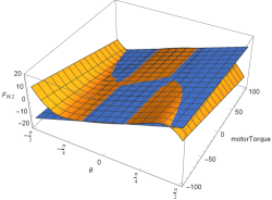
(a) horizontal force on the wheel

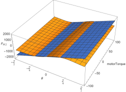
(b) torque on the saddle

Figure 3: The dependency of the physical forces on the angle $\theta$ and the motor’s force $\mathit{motorTorque}$ for a model with exemplary parameters (orange) and a linearised version thereof (blue).

SpaceEx can only analyse systems with linear behaviour [5]. We conclude that while our full model cannot be analysed with it, there are linearised versions with only reasonable errors within the range of angles $\theta$ that is most relevant to analysis.

6 Simulation

To allow easy experimentation with different approaches for controller design without having to model them as an HIOA that is amenable to formal analysis, we developed a simulation framework in Mathematica. It approximates the model’s behaviour for a concrete controller and user input using digital time.

Figure 4: The order of evaluation in the simulation framework.

Figure 4 shows the core of the simulation algorithm. To visualize the result, the framework can generate graphs plotting certain model parameters as well as animations displaying the state of the unicycle and the forces acting on it over time. Figure 1 has been generated using this framework.

7 Conclusion

This paper has developed a model of a unicycle where pedals are used for both power generation and speed control. We have discussed simplifications needed to make the model amenable to verification, and have presented a simple simulation environment.

Additional Resources.

Additional materials such as model files and the simulation framework can be found at http://depend.cs.uni-saarland.de/~freiberger/unicycles/, also including animations and an implementation of a PID-based controller.

Acknowledgements.

The authors are grateful to Felix Maurer for double-checking the physics, and to the contributors to the discussion “Movement and Rotation of a Inverted-Pendulum-like Object with External Forces”.

Appendix A Physics of a Unicycle

In this appendix, we justify and explain the derivations in Section 2.1.

A.1 Abstracting Away the Moment of Inertia of the Wheel

For a moment, let us just consider the wheel $W$. If it is moving, it is both rotating around its center and translating along the ground. If a horizontal force $F$ is acting on it, its effect is governed by both the inertia and moment of inertia of $W$.

We will now derive the movement equations as in [6] for $W$ under such an external force $F$, yielding a way to simplify the model.

Figure 5: Wheel $W$ with an External Force $F$

The system is sketched in Figure 5. The external force $F$ affects the center of mass of the wheel. The static friction between the wheel and the ground causes a force $F_{s}$ that is pulling the bottom of the wheel against the direction of $F$.

We will call the linear acceleration of $W$ to the left $a$, and the counterclockwise angular acceleration $\alpha$. Therefore, we have:

$$F-F_{s} =m_{W,\mathit{real}}\cdot a$$ (1)

$$F_{s}\cdot r_{W} =I_{W}\cdot\alpha$$ (2)

Since the wheel is not slipping, we can relate $a$ and $\alpha$:

$$\alpha=\frac{a}{r_{W}}$$ (3)

By substituting Equation 3 in Equation 2, we obtain:

$$F_{s}=I_{W}\cdot\frac{a}{r_{W}^{2}}$$ (4)

By substituting this in Equation 1, we obtain:

$$a=\frac{F}{m_{W,\mathit{real}}+\frac{I_{W}}{r_{W}^{2}}}$$ (5)

The moment of inertia $I$ depends on the mass distribution in $W$. If it is distributed evenly in a cylindrical wheel, we have $I=\frac{1}{2}\cdot m_{W,\mathit{real}}\cdot r_{W}^{2}$; if the mass is only in the outermost points (effectively making the wheel a ring), we have $I=m_{W,\mathit{real}}\cdot r_{W}^{2}$. In reality, the mass distribution will be somewhere in between, leading to

$$I=\xi\cdot m_{W,\mathit{real}}\cdot r_{W}^{2}$$ (6)

for a $\xi\in[0.5,1]$.

By substituting Equation 6 in Equation 5, we finally obtain:

$$a=\frac{F}{m_{W,\mathit{real}}+\xi\cdot m_{W,\mathit{real}}}$$ (7)

Coincidentally, this equation also describes the frictionless acceleration of an object with the mass

$$m_{W}\coloneqq m_{W,\mathit{real}}+\xi\cdot m_{W,\mathit{real}}.$$ (8)

In the following sections, we will therefore neglect any rotational forces on $W$ and use the adjusted mass $m_{W}$ to accommodate them instead.

A.2 From External Torque to a Linear Force

We can now think of the unicycle as a point of mass $W$ that slides frictionless along a surface, with the rod $S$ mounted on it. Since the external torque $\tau_{W,\mathit{mot}}$ is rotating $W$ counterclockwise using a moment arm of length $r_{W}$, we can view it as a force $F_{W,\mathit{mot}}$ that is pulling $W$ to the right with

$$F_{W,\mathit{mot}}=-\frac{-\tau_{W,\mathit{mot}}}{r_{W}},$$ (9)

as shown in Figure 6 (where $F_{W,\mathit{mot}}$ is negative and therefore points to the left).

Figure 6: Converting $\tau_{W,\mathit{mot}}$ to $F_{W,\mathit{mot}}$

A.3 Adding Gravity

Now, we will factor in gravity. We do not need to consider the effect of gravity on $W$ – it only affects the friction between $W$ and the ground, and we already assumed that $W$ does not slip. However, gravity also has an affect on $S$: If $S$ is not upright, it creates a torque on it. The situation is sketched in Figure 7.

(a) The First Split

(b) The Second Split

Figure 7: The Effect of Gravity on $S$

The gravitational pull of strength $F_{g}=m_{s}\cdot g$ acts on the center of mass of $S$. It can be split into two parts. One of them causes a torque $\tau_{S,g}$ with a moment arm of length $r_{\mathit{com}}$. The other part pulls along the rod, towards the wheel. At the wheel, this force is split once again, into a part that is perpendicular to the ground and can be ignored, and a force $F_{W,g}$ that pushes $W$ to the right. By the geometry of the unicycle, we can compute the strength of these forces:

$$\tau_{S,g} =m_{s}\cdot g\cdot\sin\theta\cdot r_{\mathit{com}}$$ (10)

$$F_{W,g} =m_{s}\cdot g\cdot\cos\theta\cdot\sin\theta$$ (11)

We now have derived two forces pushing on $W$ to the right: $F_{W,\mathit{mot}}$ caused by the driver or motor and $F_{W,g}$ caused by gravity. We call the sum of both forces $F_{W}$:

$$F_{W}=F_{W,\mathit{mot}}+F_{W,g}$$ (12)

While $F_{W}$ is the only force that acts on $W$ horizontally, this still is not enough to describe the motion of $W$, since $W$ and $S$ are connected and $S$ is free to rotate. We will analyze the effects of such a force in the next section.

A.4 Splitting an External Linear Force on $W$ and $S$

We will now derive the equations for a unicycle where an external force $F_{W}$ acts on the wheel as depicted in 8(a). For this consideration, we will assume that no other forces act on the system.

(a) $F_{W}$ acts on the Unicycle

(b) $F_{W,2}$ and an Isolated $W$

(c) $F_{W,1}$ and an Isolated $S$

Figure 8: Splitting an External Force

We consider the effects on $W$ and on $S$ separately. The part of the force that only affects the wheel will be called $F_{W,2}$, the part that only affects $S$ will be called $F_{W,1}$. We know that

$$F_{W}=F_{W,1}=F_{W,2}$$ (13)

must hold. We consider the effect of $F_{W,2}$ on a wheel (see 8(b)) and the effect of $F_{W,1}$ on $S$ (see 8(c)) in isolation, assuming that the lower end of $S$ may not move up or down.

For the scenario in 8(b), we can easily compute the acceleration of $W$:

$$a_{W}=\frac{F_{W,2}}{m_{W}}$$ (14)

In the scenario in 8(c), the force $F_{W,1}$ is acting on an object that can both rotate around its center of mass and translate linearly. In this case, both things happen, and we can compute both the linear and angular acceleration:

$$a_{S} =\frac{F_{W,1}}{m_{S}}$$ (15)

$$\alpha_{S} =\frac{r_{\mathit{com}}\cdot F_{W,1}\cdot\cos\theta}{I_{S}}$$ (16)

Since the lower end of $S$ is fixed to $W$, we know that their acceleration is the same:

$$a_{S}+\alpha_{S}\cdot r_{\mathit{com}}\cdot\cos\theta=a_{W}$$ (17)

From this, we immediately obtain the ratio of the two forces, which we will call $\beta$:

$$\beta\coloneqq\frac{F_{W,1}}{F_{W,2}}=\frac{m_{S}}{m_{W}}\cdot\left(1+3\cos^{2}\theta\right)$$ (18)

This allows us to finally quantify both parts of $F_{W}$:

$$F_{W,1} =F_{W}\cdot\frac{\beta}{1+\beta}$$ (19)

$$F_{W,2} =F_{W}\cdot\frac{1}{1+\beta}$$ (20)

A.5 Torque on $S$ by Linear Acceleration

The force $F_{W,1}$ accelerates the bottom end of $S$ to the right. This causes both linear acceleration which we can ignore since $S$ is fixed to $W$, and rotation around the center of mass. By the geometry of the unicycle, we can quantify this torque $\tau_{S,W}$:

$$\tau_{S,W}=F_{W,1}\cdot r_{\mathit{com}}\cdot\cos\theta$$ (21)

Therefore, we know all torques affecting $S$, and can compute the total torque on $S$:

$$\tau_{S}=-\tau_{W,\mathit{mot}}+\tau_{S,g}+\tau_{S,W}$$ (22)

A.6 Flow Equations

Now, we can finalize our model by specifying how the position $x_{W}$ of the wheel and the angle $\theta$ of the saddle evolve:

$$\dot{x_{W}} =v_{W}$$ (23)

$$\dot{v_{W}} =\frac{F_{W,2}}{m_{W}}$$ (24)

$$\dot{\theta} =\omega$$ (25)

$$\dot{\omega} =\frac{\tau_{S}}{I_{S}}$$ (26)

References

- [1]
- [2] Rajeev Alur, Costas Courcoubetis, Nicolas Halbwachs, Thomas A. Henzinger, Pei-Hsin Ho, Xavier Nicollin, Alfredo Olivero, Joseph Sifakis & Sergio Yovine (1995): The Algorithmic Analysis of Hybrid Systems. Theor. Comput. Sci. 138(1), pp. 3–34. Available at http://dx.doi.org/10.1016/0304-3975(94)00202-T.
- [3] Alexandre Donzé & Goran Frehse (2013): Modular, Hierarchical Models of Control Systems in SpaceEx. In: Proc. European Control Conf. (ECC’13), Zurich, Switzerland.
- [4] Qing Feng & Kazuo Yamafuji (1988): Design and simulation of control systems of an inverted pendulum. Robotica 6(3), pp. 235–241. Available at http://dx.doi.org/10.1017/S0263574700004343.
- [5] Goran Frehse, Colas Le Guernic, Alexandre Donzé, Scott Cotton, Rajarshi Ray, Olivier Lebeltel, Rodolfo Ripado, Antoine Girard, Thao Dang & Oded Maler (2011): SpaceEx: Scalable Verification of Hybrid Systems. In Ganesh Gopalakrishnan & Shaz Qadeer, editors: Computer Aided Verification - 23rd International Conference, CAV 2011, Snowbird, UT, USA, July 14-20, 2011. Proceedings, Lecture Notes in Computer Science 6806, Springer, pp. 379–395. Available at http://dx.doi.org/10.1007/978-3-642-22110-1_30.
- [6] D. Halliday, R. Resnick & J. Walker (2013): Fundamentals of Physics Extended, 10th Edition. Wiley Global Education. Available at https://books.google.de/books?id=DTccAAAAQBAJ.
- [7] Teun van Kuppeveld (2007): Model-based redesign of a self-balancing scooter. Available at http://essay.utwente.nl/790/.