RUP-15-25
Gravitational two solitons in Levi-Cività spacetime
Abstract
Applying the Pomeransky inverse scattering method to the four-dimensional vacuum Einstein equations and using the Levi-Cività solution as a seed, we construct a two-soliton solution with cylindrical symmetry. In our previous work, we constructed the one-soliton solution with a real pole and showed that the singularities that the Levi-Cività background has on an axis can be removed by the choice of certain special parameters, but it still has unavoidable null singularities, as usual one-solitons do. In this work, we show that for the two-soliton solutions, any singularities can be removed by suitable parameter-setting and such solutions describe the propagation of gravitational wave packets. Moreover, in terms of the two-soliton solutions, we mention a time shift phenomenon, the coalescence and the split of solitons as the nonlinear effect of gravitational waves.
pacs:
04.20.Jb, 04.30.-wI Introduction
Gravitational solitons in general relativity describe gravitational solitonic waves propagating in a certain background spacetime. In particular, the use of inverse scattering method leads to a lot of discoveries of various physically interesting exact solutions book exact solution ; Belinski:2001ph . It should be especially mentioned that, in addition to exact solutions describing nonlinear gravitational waves on various physical backgrounds, this method can generate black hole solutions in an axisymmetric and stationary case, and multiple-soliton solutions with stationary and axial symmetry, such as the generalized soliton solutions of the Weyl class, Kerr-NUT solutions, double Kerr metric, and the rotating Weyl -metric etc. Belinski:2001ph ; Letelier:1985 ; Carot:1989it ; Chaudhuri:1997 . This method can be generalized to the higher-dimensional Einstein equations Iguchi:2011qi ; review ER , but in general such a simple generalization to higher dimensions tends to lead to singular solutions. However, Pomeransky Pomeransky:2005sj modified the original inverse scattering method Belinsky:1979mh so that it can generate regular solutions even in higher dimensions. In fact, with regard to vacuum solutions in five dimensions, all currently known asymptotically flat black hole solutions can be discovered or rederived by this method Iguchi:2011qi ; review ER .
In a cylindrically symmetric case, a diagonal form of a metric makes the vacuum Einstein equations extremely simple structure of a linear wave equation in a flat background. For instance, the Einstein-Rosen metric can be interpreted as superposition of cylindrical gravitational waves with the mode only Einstein-Rosen ; book exact solution . However, the existence of off-diagonal nonzero components of a metric drastically changes the structure of the Einstein equations and it yields the mode together with nonlinearity. Piran et al. Piran numerically studied the nonlinear interaction of cylindrical gravitational waves with both polarization modes such as the gravitational Faraday effect. Tomimatsu Tomimatsu:1989vw studied the gravitational Faraday rotation for the cylindrical gravitational solitons generated by the inverse scattering technique Belinsky:1979mh . As one of new attempts to understand strong gravitational effects, one of the present authors has recently constructed the cylindrically symmetric soliton solutions from a Minkowski seed by the Pomeransky inverse scattering method, and has clarified the behavior of the soliton solution including the effect similar to the gravitational Faraday rotation Tomizawa:2013soa ; Tomizawa:2015zva .
In our previous paper, using the Pomeransky inverse scattering method and regarding the Levi-Cività metric as a seed, we constructed the one-soliton solution that does not admit staticity but cylindrical symmetry Igata:2015oea . Although Levi-Cività spacetime has singularities on the axis except for Minkowski spacetime, we showed that for the one-soliton solution, such singularities disappear by a certain choice of parameters. However, this solution has singularities on the light cone for any parameters, which is an unavoidable common property for all one-soliton solutions with a real pole and it is well known that such a problem can be resolved by considering two-soliton solutions with two complex-conjugate poles. Therefore, in this paper, we will construct a two-soliton solution with two complex conjugate poles by the Pomeransky method and the Levi-Cività seed. Furthermore, we will show that for certain parameters, the spacetime is entirely free from any singularities even on the axis as well as on the light cone.
In the following section, we will present a two-soliton solution with complex conjugate poles in Levi-Cività spacetime. In Sec. III we will analyze the obtained two-soliton solution by computing the amplitudes and polarization angles for ingoing and outgoing waves and will see the difference from the one-soliton solution. In Sec. IV, we will give the summary and discussion on our results.
II Two-soliton solution
The most general cylindrically symmetric solution to the four-dimensional vacuum Einstein equations can be described in the Kompaneets-Jordan-Ehlers form Komaneets-Jordan-Ehlers
| (1) |
where the functions , , and depend on the time coordinate and radial coordinate only. Let us define a metric and a metric function by
| (4) | |||
| (5) |
respectively.
As shown by Belinsky and Sakharov Belinsky:1979mh , the vacuum Einstein equation with cylindrical symmetry (in general, with two commuting Killing vectors) is completely integrable, and it admits a pair of linear equations, which is called Lax pair
| (6) |
where is a spectral parameter (complex parameter), and are the commuting differential operators defined by
| (7) |
and and are the matrices defined by and , respectively, and the generating matrix is a matrix such that . Therefore, one can obtain the metric from the generating matrix (more precisely, by normalizing the metric such that ).
To generate new cylindrically symmetric solutions, we start from one solution of the Lax pair such that ( : a seed metric) and then must dress it as
| (8) |
where in particular, for a two-soliton solution, the dressing matrix is given by
| (9) |
with
| (10) | |||
| (11) | |||
| (12) |
where, following the notation in Belinski:2001ph , we use the successive Latin subscripts to denote the summation of the and components, and are defined by
| (13) |
The constant vectors add the seed to new parameters (the obtained solution is invariant under the transformation (: a nonzero constant)). After dressing, taking the limit of , one can obtain the metric . In the Belinsky-Zakarov method, one must normalize the obtained metric. Furthermore, for reality of the metric, one must put .
In this paper, following the Pomeransky method Pomeransky:2005sj , in which one need not normalize the metric obtained from the dressed generating matrix. For the Levi-Cività metric, which we choose as a seed, the metric and the metric function are written as
| (14) | |||
| (15) |
respectively, where the parameters and are independent, and are assumed to be positive without loss of generality. Let us remove trivial solitons at and with a vector (this corresponds to the inverse transformation with in the Belinski-Zakharov method), and then we have the metric
| (16) |
and dress the generating matrix corresponding to the metric :
| (17) |
where
| (18) |
Next, add back nontrivial solitons with BZ vectors and , and then we obtain a two-soliton solution as
| (19) | |||
| (20) |
where is evaluated at .
This is how we can obtain a two-soliton solution, whose metric can be written in the Kompaneets-Jordan-Ehlers form (1), where the functions , and are explicitly written as
| (21) | |||
| (22) | |||
| (23) |
with111 The function can be rewritten in terms of and as
| (24) | |||
| (25) | |||
| (26) |
| (27) | |||
| (28) | |||
| (29) | |||
| (30) |
Here, denotes the real part of . When , we recover the metric in Tomizawa:2015zva , in which case the seed is a Minkowski metric, and when , this metric reduces to the Levi-Cività metric.
A shift of the time coordinate allows us to fix the parameters as a pure imaginary
| (31) |
where denotes the imaginary unit and is assumed to be positive without loss of generality.
III Analysis for two-solitons
III.1 Asymptotic behaviors of gravitational waves
In this subsection, we analyze the asymptotic behaviors of gravitational waves at spacetime boundaries for the obtained two-soliton solution by computing the asymptotic behaviors of the metric and ingoing and outgoing wave amplitudes, where we basically follow the definitions given in Refs. Piran ; Tomimatsu:1989vw (see Appendix A). First, let us consider the symmetric axis . In order to focus on the physical propagation process of cylindrically symmetric gravitational soliton waves, we investigate the condition for the parameters and such that there do not exist any gravitational sources on the axis, i.e., the C-energy density could become finite on the axis.
Note that the C-energy density is proportional to . Near , the metric function behaves asymptotically as
| (32) |
where denotes the imaginary part of .
For , the C-energy density diverges on as
| (33) |
but for , it vanishes as
| (34) | ||||
| (35) | ||||
| (36) |
where we assume for because if not, diverges on . The case of (two-soliton solution obtained from Minkowski metric) have been previously analyzed by one of the authors Tomizawa:2015zva . This is why we focus on and only in what follows.
Near , the metric behaves as
| for | (37) | |||||
| for | (38) | |||||
where we have introduced the new coordinates and for . A deficit angle on the axis is defined as
| (39) |
where is replaced by for , and is the periodicity of the angular coordinate. Then we have
| (40) | ||||
| (41) |
By choosing a suitable value of to be , we get rid of conical singularities on the axis.
Near , the ingoing and outgoing total amplitudes, and , behave as
| (42) | ||||
| (43) |
respectively. The polarization angles, and , take the following asymptotic forms
| (44) | |||||
| (45) | |||||
At late time or at early time , the metric behaves as
| (46) | |||||
| (47) |
The total amplitudes and polarization angles behave as
| (48) | ||||
| (49) |
and
| (50) | ||||
| (51) |
At spacelike infinity , the metric behaves as
| (52) | |||||
| (53) |
The total amplitudes and polarization angles behave as
| (54) | ||||
| (55) |
and
| (56) | ||||
| (57) |
At past null infinity , the metric behaves as
| (58) | ||||
| (59) |
where and are defined by
| (60) | ||||
| (61) | ||||
| (62) |
The asymptotic forms of the amplitudes and the polarization angles are
| (63) | |||
| (64) |
where
| (65) | ||||
| (66) | ||||
| (67) | ||||
| (68) |
and
| (69) |
At future null infinity , the metric behaves as
| (70) | ||||
| (71) |
where and are defined by
| (72) | ||||
| (73) | ||||
| (74) |
The asymptotic forms of the amplitudes and the polarization angles are
| (75) | |||
| (76) |
where and are defined by
| (77) | ||||
| (78) | ||||
| (79) | ||||
| (80) | ||||
| (81) |
and
| (82) |
III.2 Wave propagation
 |
 |
 |
 |
 |
 |
(a)

(b)
 |
 |
 |
 |
 |
 |
(a)


(b)
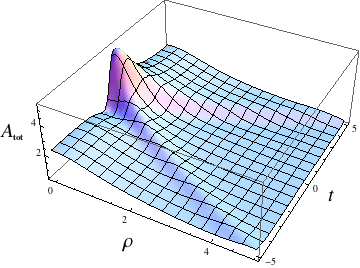
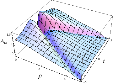
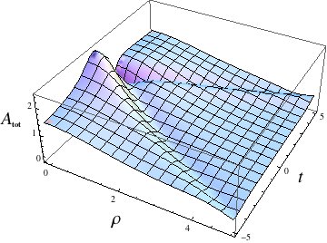
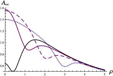
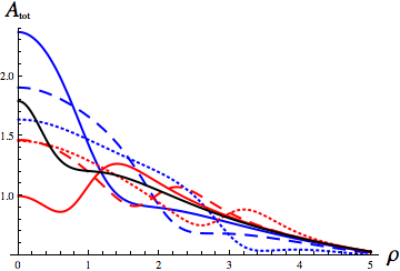
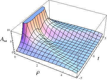
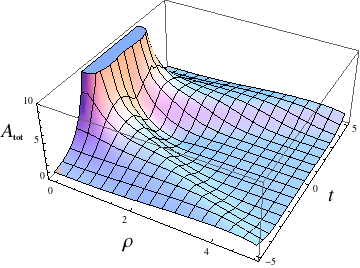
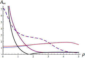
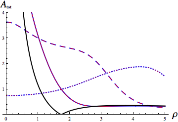
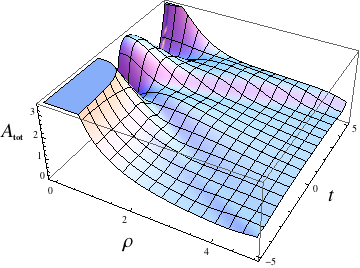
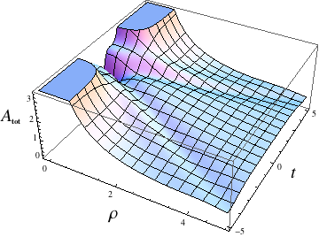
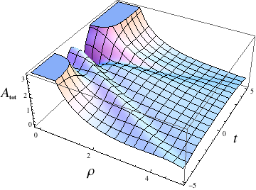
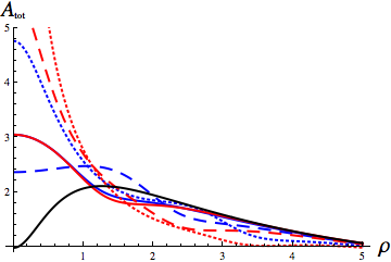
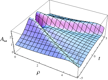
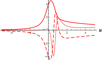
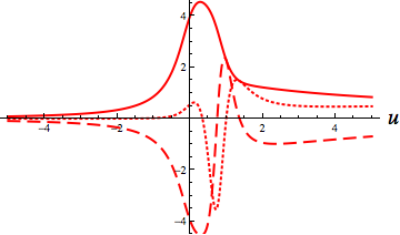
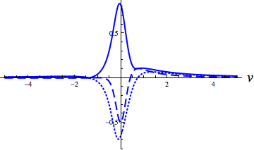
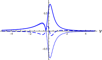
Let us see the qualitative behavior of the gravitational waves described by the obtained two-soliton solution near the axis . Figures 1 and 2 display the typical wave forms and their snapshots of the total amplitudes, , near the coordinate origin for and , respectively, where we specify by two real parameters and as
| (83) |
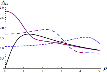
and moreover we set . In each figure, we consider the three cases only to see the typical picture of reflection. Both figures explicitly show that the obtained two-soliton solution describes the reflectional phenomenon of cylindrical gravitational waves. For , the solution provides the picture of soliton reflection near as seen in Figs. 1(a) and 2(a). Note that for , becomes larger and larger near the axis as increases in Fig. 2(a). For , the dependence of on is quite small as seen in Figs. 1(b) and 2(b). From these behaviors of the amplitudes, we may consider that the two-soliton solutions show the propagation of gravitational wave packets which first come into the symmetric axis from past null infinity , and leave the axis after reflection for future null infinity .
III.3 Time shift
 |
 |
 |
 |
 |
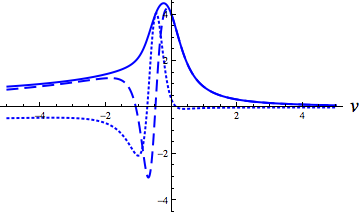 |
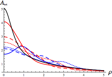
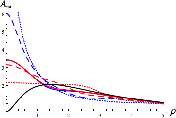
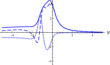
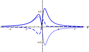
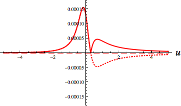
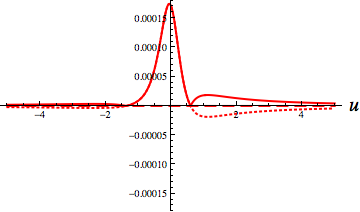
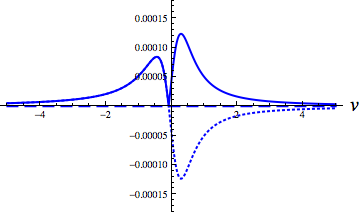
A time shift phenomenon is known as the nonlinear effect of solitons, which means that a wave packet propagates at slower speed than the light velocity by its self-interaction when a cylindrical wave collapses near the axis. Let us note that the amplitudes for ingoing waves near past null infinity [Eqs. (63) and (64)] and the amplitudes for outgoing waves near future null infinity [Eqs. (75) and (76)] have the same forms as for . Therefore, the behaviors near and for is exactly the same as for discussed in Tomizawa:2015zva . In Fig. 3, the blue-colored graphs and the red-colored graphs denote and for , respectively, where we take to see the typical behaviors of waves. The dashed and dotted blue-colored (red-colored) graphs denote and at null infinity , respectively. It is worth noting that for large value of , both amplitudes near past and future null infinity are composed of mode waves.
To see that a time shift phenomenon happens, as was already explained in Tomizawa:2015zva , let us consider the incoming massless test particle which starts from past null infinity, propagates along the null geodesic , is reflected on the axis and then propagates to future null infinity along the null geodesic . An incident wave packet has a peak near , while a reflectional wave packet has a peak at . This means that an observer at past null infinity sees an ingoing wave packet earlier than an incoming radial photon, but at future null infinity he sees the outgoing wave packet after the outgoing photon. We may consider that a gravitational wave packet can propagate at slower speed than the light velocity.
III.4 Coalescence and split of solitons
 |
 |
 |
 |
 |
 |
(a)
(b)
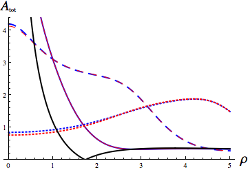
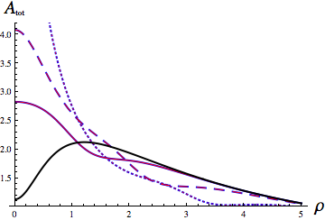
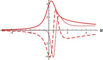
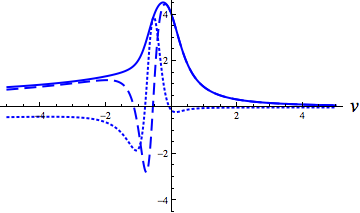
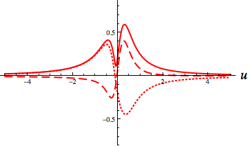
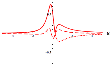
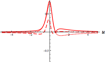
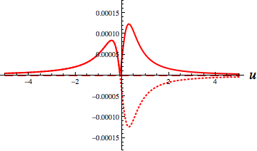
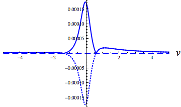
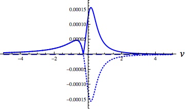
In addition to the time shift phenomena, when , physically and mathematically interesting phenomenon such as coalescence and split of solitons happens, as pointed out in Tomizawa:2015zva . As seen in Fig. 4, according to the values of , the ingoing and outgoing waves take various shapes, where the blue-colored and red-colored graphs show the ingoing amplitude at past null infinity and outgoing amplitudes at future null infinity , respectively, and the dashed and dotted graphs show the mode wave amplitudes and the mode wave amplitudes, respectively. Here, (a) and (b) in Fig. 4 are plotted for the parameters and , respectively, where we take . From these graphs, we can see that at least, either of ingoing and outgoing waves can have two peaks.
For , there are two incident wave packets, one with a small peak and another with a large peak near past null infinity, and after reflection we have two reflectional wave packets, one with a small peak and one with a large peak near future null infinity. This obviously shows that two gravitational solitons collide with each other, which occurs near the axis , and then the larger one of two solitons overtakes the smaller one (see the case in Fig. 1).
For , the incident waves incoming from past null infinity (the blue-colored graphs) have two peaks and the reflectional waves outgoing to future null infinity (the red-colored graphs) have one peak only. As seen from the case of in Fig. 1, two wave packets seem to change into one wave packet after the reflection at the axis. Therefore, this can be interpreted as the coalescence of two solitons.
In contrast to , for , the incident waves (the blue-colored graphs) have one peak near past null infinity, and the reflectional waves (the red-colored graphs) have two peaks near future null infinity. From the case in Fig. 1, one wave packet seems to change into two wave packets after the reflection at the axis. This phenomenon can be interpreted as the split of soliton waves. The phenomena of the coalescence and split do not happen for other solitons than ones in general relativity.
Finally, we comment on which polarization mode contributes to the total ingoing and outgoing amplitudes at null infinity. As seen from the behaviors of the dashed and dotted graphs in Fig. 4, for the small values of the mode only mainly contributes to both ingoing and outgoing amplitudes, while for the large values of both the and modes contribute to them to the same order.
IV Conclusions
In this paper, applying the Pomeransky method to a cylindrically symmetric spacetime and starting from the Levi-Cività background, we have constructed the two-soliton solutions with two complex conjugate poles to the vacuum Einstein equations with cylindrical symmetry. As shown in the previous work, although the Levi-Cività spacetime generally includes singularities on its axis of symmetry, for the one-soliton solution with , such singularities can be removed Igata:2015oea . In this work, we have analytically shown that as for the two-soliton solution with , singularities on an axis entirely disappear in addition to null singularities which one solitonic solution with a real pole has in common. The regular solutions with describe the propagation of gravitational wave packets that come into the region near the symmetric axis from past null infinity, then leave for future null infinity after reflection at the axis. Moreover, we have studied nonlinear effect of solitons such as a time shift phenomenon and the gravitational Faraday effect. We have seen that these effects are essentially similar to the case of , which was investigated in Tomizawa:2015zva .
Finally, we point out the essential differences of two-soliton solutions with from ones with .
(i) Axis of symmetry :
For , the C-energy density vanishes on the axis , as for , although it diverges in the Levi-Cività background spacetime. Therefore, since there does not exist any gravitational sources on the axis, the two-soliton solution can be physically interpreted as the reflection process of gravitational solitonic waves at the axis. Furthermore, at late time , for the C-energy density approaches a constant value, while for it becomes an infinitely large value.
(ii) Timelike infinity :
For , the spacetime asymptotically approaches Minkowski, and simultaneously both ingoing and outgoing gravitational waves fade into the background spacetime. The mode for the ingoing and outgoing waves becomes dominant at late time. On the other hand, for , the spacetime is not asymptotically Minkowski and both ingoing and outgoing wave amplitudes do not vanish. Moreover, for both modes are present, and for the mode becomes dominant.
(iii) Null infinity or :
Even though the asymptotic forms of the metric at null infinity entirely differ for each of , the asymptotic forms of wave packet are exactly same. Therefore, as happens for , for , two gravitational solitons can coalesce into a single soliton, and also that a single soliton can split into two via the nonlinear effect of gravitational waves. Such phenomena cannot be seen for solitons of other integrable equations such as solitons of the KdV equation.
Acknowledgements.
This work was partially supported by the Grant-in-Aid for Young Scientists (B) (No. 26800120) from Japan Society for the Promotion of Science (S.T.).Appendix A Definitions
In this Appendix, we provide the well-used definitions on the amplitudes and polarization angles of nonlinear cylindrically symmetric gravitational waves, which were first used in Piran ; Tomimatsu:1989vw .
The amplitudes of ingoing and outgoing waves with the mode are defined as, respectively,
| (84) | |||
| (85) |
and the amplitudes of ingoing and outgoing waves with the mode are defined as, respectively,
| (86) | |||
| (87) |
where the advanced ingoing and outgoing null coordinates and are defined by and , respectively. The total amplitudes of ingoing and outgoing waves are defined by
| (88) | |||
| (89) |
respectively, and moreover the total amplitude of cylindrical gravitational waves is written as
| (90) |
The polarization angles and for the respective wave amplitudes are defined as
| (91) | |||
| (92) |
The vacuum Einstein equations can be written in terms of these quantities as follows:
| (93) | |||
| (94) | |||
| (95) | |||
| (96) |
and
| (97) | |||
| (98) |
References
- (1) H. Stephani, D. Kramer, M. A. H. MacCallum, C. Hoenselaers and E. Herlt, Exact solutions of Einstein’s Field Equations, 2nd ed. (Cambridge University Press, Cambridge, 2003).
- (2) V. A. Belinski and E. Verdaguer, Gravitational Solitons, (Cambridge University Press, Cambridge, 2001).
- (3) P. S. Letelier, J. Math. Phys. 26, 467 (1985).
- (4) J. Carot and E. Verdaguer, Class. Quant. Grav. 6, 845 (1989).
- (5) S. Chaudhuri and K. Das, Gen. Rel. Grav. 29, 75 (1997).
- (6) H. Iguchi, K. Izumi, and T. Mishima, Prog. Theor. Phys. Suppl. 189, 93 (2011).
- (7) R. Emparan and H. S. Reall, Living Rev. Rel. 11, 6 (2008).
- (8) A. A. Pomeransky, Phys. Rev. D 73, 044004 (2006).
- (9) V. A. Belinsky and V. E. Sakharov, Sov. Phys. JETP 50, 1 (1979).
- (10) A. Einstein and N. Rosen, J. Franklin Inst. 223, 43 (1937).
- (11) T. Piran, P. N. Safier, and R. F. Stark, Phys. Rev. D 32, 3101 (1985).
- (12) A. Tomimatsu, Gen. Rel. Grav. 21, 613 (1989).
- (13) S. Tomizawa and T. Mishima, Phys. Rev. D 90, 044036 (2014).
- (14) S. Tomizawa and T. Mishima, Phys. Rev. D 91, 124058 (2015).
- (15) T. Igata and S. Tomizawa, Phys. Rev. D 91, 124008 (2015).
- (16) P. Jordan, J. Ehlers, and W. Kundt, Abh. Akad. Wiss. Mainz. Math. Naturwiss. Kl. 2, 16 (1960); A. S. Kompaneets, Zh. Eksp. Teor. Fiz. 34, 953 (1958) [Sov. Phys. JETP 7, 659 (1958)].