Signal amplification in a qubit-resonator system

Abstract

We study the dynamics of a qubit-resonator system, when the resonator is driven by two signals. The interaction of the qubit with the high-amplitude driving we consider in terms of the qubit dressed states. Interaction of the dressed qubit with the second probing signal can essentially change the amplitude of this signal. We calculate the transmission amplitude of the probe signal through the resonator as a function of the qubit’s energy and the driving frequency detuning. The regions of increase and attenuation of the transmitted signal are calculated and demonstrated graphically. We present the influence of the signal parameters on the value of the amplification, and discuss the values of the qubit-resonator system parameters for an optimal amplification and attenuation of the weak probe signal.

I Introduction

Quantum optical effects with Josephson-junction-based circuits have been intensively studied for the last decade. In particular, such systems are interesting as two-level artificial atoms (qubits) OmelIlShev ; Wendin ; Greenberg08 . Quantum energy levels and quantum coherence are inherent to qubits and provide the basis for studying fundamental quantum phenomena. It is important to note that qubits can be controlled over a wide range of parameters Oelsner10 ; Ashhab09 ; Wang14 ; Andersen14 ; OmelIlShev and they have unavoidable coupling to the dissipative environment.

The ability of stimulated emission and lasing in superconductive devices has been actively studied during the last several years both theoretically Shevchenko14 ; Sajko14 ; Sajko141 ; Sajko142 ; Xu14 and experimentally Oelsner13 ; Hauss08 ; Forster15 . The work is underway on using these phenomena as basis for a quantum amplifier of signals near the quantum limit. This paper was motivated by several recent publications where the amplification of the input signal was observed in systems with nanomechanical resonators Wang14 ; Hauss07 , with waveguide resonators Ashhab09 ; Hauss08 ; Oelsner13 ; Satanin14 ; Greenberg07 and the concept of the amplifiers was discussed Abdo14 ; Astafiev101 ; Lin13 ; Bergeal10 .

A key value of the qubit-resonator system in the experiment is the transmission coefficient of the signal through the resonator. This transmission coefficient depends on different parameters. The speed and direction of the energy exchange is determined by relaxation rates. The variation of the coupling strength allows to change the width of resonance. The change of the driving amplitude and the magnetic flux (for flux and PSQ qubit; for charge qubit this quantity is the applied voltage) allows to find an acceptable point on the resonance line comparative to other parameters.In the paper we consider how the amplification and attenuation of the input signal depend on the parameters of the system. The general idea is to find values and there relationship for the parameters of the system in order to make the amplification maximal.

In addition to Ref. Shevchenko14 here we systematically study the impact of such parameters as coherent time, resonator loss, coupling and other. Also we demonstrated how temperature influences the transmission coefficient. Besides we show the universality of the doubly-dressed approach for two-level systems. We compare the appearance of the amplification-attenuation phenomena in both flux and phase-slip qubit Mooij06

The paper is organized as follows Sec. II contains a description of the studied system which is a qubit coupled to the two-mode $\lambda/2$ waveguide resonator. Sec. III is devoted to the evolution of the qubit-resonator system which is described by a Lindblad equation. We analyze the solution of the Lindblad equation in Sec. IV. Sec. V concludes the paper.

II The qubit-resonator system

The studied system consists of a quantum resonator (transmission-line resonator with the length $L=\lambda/2$) and a two-level system, the superconducting flux qubit. The qubit interacts with two harmonics in the resonator: first probing signal with frequency $\omega_{\mathrm{p}}$ close to the first harmonic of the resonator and the second signal is a high amplitude driving signal with frequency $\omega_{\mathrm{d}}$ close to the third harmonic of the resonator. Such system is analogous to the one studied recently experimentally in Refs. Oelsner10 ; Astafiev12 ; Shevchenko14 .

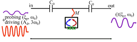
Figure 1: Diagrammatic representation of the system under study: a qubit placed in a waveguide resonator. The qubit interacts with a two-mode resonator. The first signal has an amplitude $\xi_{\mathrm{d}}$ and a frequency $\omega_{\mathrm{p}}$. The second signal has an amplitude $A_{\mathrm{d}}$ and a frequency $\omega_{\mathrm{d}}$. A measurable (probing) signal at the output has an amplitude different from the input values.

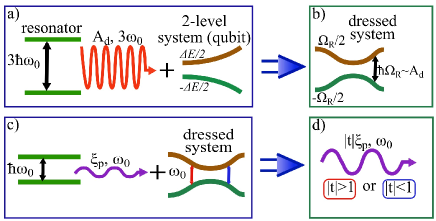
Figure 2: The interaction between a qubit and a resonator can be described in frame of the dressed states. (a) A high-amplitude signal $A_{\mathrm{d}}$ interacts with a two-level system (qubit). (b) Energy levels are modified. The qubit can be described in terms of the dressed states, in other words we obtain a dressed two-level system with energy distance proportional to the amplitude $A_{\mathrm{d}}$ of the third-harmonic. (c) The dressed qubit interacts with probe signal. (d) The amplitude of the output signal is increased or weakened.

The qubit located in the middle of the resonator ($x=0$) is coupled only to the odd harmonics $m$, for which the current is defined by $I(x)=I_{{m}}\cos\pi mx/L$ (see Fig. 1). The transmission-line resonator runs from $-L/2$ to $L/2.$ We consider the interaction of the qubit and two-mode resonator according to doubly-dressed approach, as in Ref. Shevchenko14 . Hamiltomian of the system is

$$H_{\mathrm{tot}} = \hbar\frac{\delta\widetilde{\omega}_{\mathrm{qb}}}{2}\widetilde{\sigma}_{z}+\hbar\delta\omega_{\mathrm{r}}a^{{\dagger}}a+$$

$$+\hbar\widetilde{\mathrm{g}}\left(a\widetilde{\sigma}^{{\dagger}}\!+\!a^{{\dagger}}\widetilde{\sigma}\right)+\xi_{\mathrm{p}}\!\left(a\!+\!a^{{\dagger}}\right),$$

where $\widetilde{\sigma}_{z},$ $\widetilde{\sigma}_{x},$ $\widetilde{\sigma}_{y}$, $\widetilde{\sigma}=\frac{1}{2}(\widetilde{\sigma}_{x}-i\widetilde{\sigma}_{y})$ are the Pauli’s operators in the doubly-dressed basis; $\delta\widetilde{\omega}_{\mathrm{qb}}=\widetilde{\Delta E}/\hbar-\omega_{\mathrm{p}}$  is the detuning of the doubly-dressed qubit; $\widetilde{\Delta E}=\sqrt{\tilde{\varepsilon}^{2}+\tilde{\Delta}^{2}}=$ $\hbar\Omega_{R}$ is the Radi frequency of the dressed qubit; $\widetilde{\mathrm{g}}=\mathrm{g}_{1}\frac{\varepsilon_{0}}{\Delta E}\frac{\widetilde{\Delta}}{\widetilde{\Delta E}}$ is the renormalized coupling; $\Delta E=$ $\sqrt{\varepsilon_{0}^{2}+\Delta^{2}}$; $\varepsilon_{0}=2I_{p}\Phi_{0}\left(\Phi_{x}/\Phi_{0}-0.5\right)$where $\Phi_{x}$ is the external magnetic flux applied to the qubit loop; $I_{\mathrm{p}}$ is the persistent current in the qubit loop; $\Phi_{0}$ is the flux quantum; $\ \Delta$is the energy separation between two levels at the degeneracy point $\varepsilon_{0}=0$; $\delta\omega_{\mathrm{r}}=\omega_{\mathrm{r}}-\omega_{\mathrm{p}}$ is the detuning of the resonator; $A_{\mathrm{d}}=4\sqrt{\langle N\rangle}\hbar\mathrm{g}_{\mathrm{3}}$ is the normalized amplitude of the driving signal, given by the average number of photons $N$ in resonator of the third harmonic. The dressed bias $\widetilde{\varepsilon}$ and the tunneling amplitude $\widetilde{\Delta}$ are defined by the driving frequency $\omega_{\mathrm{d}}\$and amplitude $A_{\mathrm{d}}$ either in the weak-driving regime, at $A_{\mathrm{d}}<\hbar\omega_{\mathrm{d}}$,

$$\widetilde{\varepsilon}=\Delta E-\hbar\omega_{\mathrm{d}},\widetilde{\Delta}=\Delta A_{\mathrm{d}}/2\Delta E,$$ (2)

or in the strong-driving regime, where the energy bias is defined by the detuning from the $k$-photon resonance, $\widetilde{\varepsilon}\rightarrow\widetilde{\varepsilon}^{(k)}$, and the renormalized tunneling amplitude is defined by the oscillating Bessel function, $\widetilde{\Delta}\rightarrow\widetilde{\Delta}^{(k)}$, as following

$$\widetilde{\varepsilon}^{(k)}=\Delta E-k\hbar\omega_{\mathrm{d}},\text{ }\widetilde{\Delta}^{(k)}=\Delta\frac{k\hbar\omega_{\mathrm{d}}}{\varepsilon_{0}}J_{k}\left(\frac{A_{\mathrm{d}}}{\hbar\omega_{\mathrm{d}}}\frac{\varepsilon_{0}}{\Delta E}\right).$$ (3)

In the doubly-dressed representation the Hamiltonian (II) is written for the energy states $|0\rangle$ and $|1\rangle$, where we omitted constants terms; we have used the rotating-wave approximation. In Fig. 2 we explain the processes which take place in the qubit-resonator system.

III Evolution of the system

One possible method to describe the evolution of an open system is a solution of the Lindblad equation. In our case we rewrite it in the dressed basis similar to Ref. Shevchenko14 and take into account finite temperature Scully97 :

$$\frac{d}{dt}\widetilde{\rho} = -\frac{i}{\hbar}[H_{\mathrm{tot}},\widetilde{\rho}]+\sum\limits_{i}\widetilde{\Lambda}_{i}[\widetilde{\rho}],$$ (4)

$$\widetilde{\Lambda}_{\downarrow}[\widetilde{\rho}] = \widetilde{\Gamma}_{\downarrow}\left(\widetilde{\sigma}\widetilde{\rho}\widetilde{\sigma}^{{\dagger}}-\frac{1}{2}\left\{\widetilde{\sigma}^{{\dagger}}\widetilde{\sigma},\widetilde{\rho}\right\}\right),$$ (5)

$$\widetilde{\Lambda}_{\uparrow}[\widetilde{\rho}] = \widetilde{\Gamma}_{{}_{\uparrow}}\left(\widetilde{\sigma}^{{\dagger}}\widetilde{\rho}\widetilde{\sigma}-\frac{1}{2}\left\{\widetilde{\sigma}\widetilde{\sigma}^{{\dagger}},\widetilde{\rho}\right\}\right),$$ (6)

$$\widetilde{\Lambda}_{\phi}[\widetilde{\rho}] = \frac{\Gamma_{\phi}}{2}\left(\widetilde{\sigma}_{z}\widetilde{\rho}\widetilde{\sigma}_{z}-\widetilde{\rho}\right),$$ (7)

$$\widetilde{\Lambda}_{\kappa}[\widetilde{\rho}] = \kappa\left(\bar{n}_{th}+1\right)\left(a\tilde{\rho}a^{{\dagger}}-\frac{1}{2}\left\{a^{{\dagger}}a,\tilde{\rho}\right\}\right)+$$

$$+\kappa\bar{n}_{th}\left(a^{{\dagger}}\tilde{\rho}a-\frac{1}{2}\left\{aa^{{\dagger}},\tilde{\rho}\right\}\right),$$

$$\widetilde{\Gamma}_{\downarrow} = \Gamma_{1}\bar{n}_{th}\frac{1}{4}\left(1-\frac{\tilde{\varepsilon}}{\widetilde{\Delta E}}\right)^{2}+$$

$$+\Gamma_{1}\left(\bar{n}_{th}+1\right)\frac{1}{4}\left(1+\frac{\tilde{\varepsilon}}{\widetilde{\Delta E}}\right)^{2}+\frac{\Gamma_{\phi}}{2}\left(\frac{\tilde{\Delta}}{\widetilde{\Delta E}}\right)^{2},$$

$$\widetilde{\Gamma}_{\uparrow} = \Gamma_{1}\bar{n}_{th}\frac{1}{4}\left(1+\frac{\tilde{\varepsilon}}{\widetilde{\Delta E}}\right)^{2}+$$

$$+\Gamma_{1}\left(\bar{n}_{th}+1\right)\frac{1}{4}\left(1-\frac{\tilde{\varepsilon}}{\widetilde{\Delta E}}\right)^{2}+\frac{\Gamma_{\phi}}{2}\left(\frac{\tilde{\Delta}}{\widetilde{\Delta E}}\right)^{2},$$

$$\widetilde{\Gamma}_{\phi} = \Gamma_{1}\left(2\bar{n}_{th}+1\right)\frac{1}{2}\left(\frac{\tilde{\Delta}}{\widetilde{\Delta E}}\right)^{2}+\Gamma_{\phi}\left(\frac{\tilde{\varepsilon}}{\widetilde{\Delta E}}\right)^{2}.$$ (11)

where $\bar{n}_{th}^{-1}=\exp[\frac{\hbar\nu_{k}}{k_{B}T}]-1$ is the thermal photon number in the resonator; $\nu_{k}$ is density frequency distribution for thermal photons; $k_{B}$ is Boltzmann constant; $T$ is thermodynamic temperature of the system; $\widetilde{\rho}$ is the density matrix; $\widetilde{\Lambda}_{\phi}[\widetilde{\rho}]$ is the dressed phase relaxation of the dressed qubit; $\Gamma_{1}$ and $\Gamma_{\phi}$ are the qubit relaxation and dephasing rates; $\widetilde{\Lambda}_{\downarrow}[\widetilde{\rho}]$ is the relaxation from $|0\rangle$ to $|1\rangle$ level; $\widetilde{\Lambda}_{\uparrow}[\widetilde{\rho}]$ is the excitation from $|1\rangle$ to $|0\rangle$ level. The analysis of the difference between the rates $\widetilde{\Lambda}_{\uparrow}[\widetilde{\rho}]$ and $\widetilde{\Lambda}_{\downarrow}[\widetilde{\rho}]$ shows availability of the inverse population in the system (Figs. 4 and 8). The equation of motion for the expectation value of any quantum operator $A$:

$$\frac{d\langle A\rangle}{dt}=-\frac{i}{\hbar}\langle[A,H_{tot}]\rangle+Tr(AH_{tot}\sum\limits_{i}\widetilde{\Lambda_{i}}[\widetilde{\rho}]),$$ (12)

where $\langle A\rangle=Tr(A\rho)$, $\langle[A,H]\rangle=Tr([A,H]\rho)$, the trace is over all eigenstates of the system; and here $H$ is the Hamiltonian of the system in the doubly-dressed basis Eq. (II). For the expectation values of the operators $a,$ $a^{{\dagger}},$ $\widetilde{\sigma}^{{\dagger}},$ $\widetilde{\sigma},$ and $\widetilde{\sigma}_{z}$ we obtain the so-called Maxwell-Bloch equations:

$$\frac{d\left\langle a\right\rangle}{dt} = -i\delta\omega_{\mathrm{r}}^{\prime}\left\langle a\right\rangle-i\widetilde{\mathrm{g}}\left\langle\widetilde{\sigma}\right\rangle-i\frac{\xi_{\mathrm{p}}}{\hbar},$$ (13)

$$\frac{d\left\langle\widetilde{\sigma}\right\rangle}{dt} = -i\delta\widetilde{\omega}_{\mathrm{qb}}^{\prime}\left\langle\widetilde{\sigma}\right\rangle+i\widetilde{\mathrm{g}}\left\langle a\widetilde{\sigma}_{z}\right\rangle,$$ (14)

$$\frac{d\left\langle\widetilde{\sigma}_{z}\right\rangle}{dt} = -i2\widetilde{\mathrm{g}}\left(\left\langle a\widetilde{\sigma}^{{\dagger}}\right\rangle-\left\langle a^{{\dagger}}\widetilde{\sigma}\right\rangle\right)-$$

$$-\widetilde{\Gamma}_{+}\left\langle\widetilde{\sigma}_{z}\right\rangle-\widetilde{\Gamma}_{-},$$

where

$$\widetilde{\Gamma}_{\pm} = \left(\widetilde{\Gamma}_{\downarrow}\pm\widetilde{\Gamma}_{\uparrow}\right),$$ (16)

$$\delta\omega_{\mathrm{r}}^{\prime} = \delta\omega_{\mathrm{r}}-i\kappa/2,$$ (17)

$$\delta\widetilde{\omega}_{\mathrm{qb}}^{\prime} = \delta\widetilde{\omega}_{\mathrm{qb}}-i\widetilde{\Gamma}_{2}.$$ (18)

The Eqs. (13)-(III) were solved in our previous work Shevchenko14 in the small photon number limit ($\langle n\rangle\ll 1$).  In general, the system of equations is infinite, but it may be factorized $\langle aa^{{\dagger}}\rangle=\left\langle a\right\rangle\left\langle a^{{\dagger}}\right\rangle$ etc. This approximation can be used in the limit of strong perturbation, when the average number of photons in the system is substantially greater than unity ($\langle n\rangle\gg 1$). In this way, we simplify Eqs. (13)-(III):

$$\left\langle a\right\rangle = -\frac{\xi_{\mathrm{p}}}{\hbar}\frac{\delta\widetilde{\omega}_{\mathrm{qb}}^{\prime}}{\left\langle\widetilde{\sigma}_{z}\right\rangle\widetilde{\mathrm{g}}^{2}+\delta\widetilde{\omega}_{\mathrm{qb}}^{\prime}\delta\omega_{\mathrm{r}}^{\prime}},$$ (19)

$$\left\langle a^{{\dagger}}\right\rangle = -\frac{\xi_{\mathrm{p}}}{\hbar}\frac{\delta\widetilde{\omega}_{\mathrm{qb}}^{\prime\ast}}{\left\langle\widetilde{\sigma}_{z}\right\rangle\widetilde{\mathrm{g}}^{2}+\delta\widetilde{\omega}_{\mathrm{qb}}^{\prime\ast}\delta\omega_{\mathrm{r}}^{\prime\ast}},$$ (20)

$$\widetilde{\Gamma}_{+}\left\langle\widetilde{\sigma}_{z}\right\rangle+\widetilde{\Gamma}_{-} = 2i\frac{\xi_{\mathrm{p}}}{\hbar}\left(\left\langle a\right\rangle-\left\langle a^{{\dagger}}\right\rangle\right)+2\kappa\left\langle a\right\rangle\left\langle a^{{\dagger}}\right\rangle.$$ (21)

The transmission amplitude of the signal is defined by the formula Scully97 ; Bishop09 ; Koshino13

$$|t|=\frac{\hbar\kappa}{2\xi_{\mathrm{p}}}|\langle a\rangle|.$$ (22)

The dynamics of the two-level system coupled to a two-mode quantum resonator can be described as the solution of the Eqs. (19)-(21) in the limit of large photon numbers in the resonator. Such description offers a satisfactory explanation of the experiments with different qubits Oelsner10 ; Astafiev12 . This is demonstrated below.

IV Amplification and attenuation of the probe signal

Consider Eqs. (19)-(21) in the limit of the weak probing signal $\xi_{\mathrm{p}}$. We obtain the asymptotic solution for $\langle\sigma_{z}\rangle$:

$$\langle\sigma_{z}\rangle_{0}=-\frac{\widetilde{\Gamma}_{-}}{\widetilde{\Gamma}_{+}}.$$ (23)

A solution can also be found in the limit of large amplitudes of the probing signal $\xi_{\mathrm{p}}$:

$$\langle\sigma_{z}\rangle_{\infty}=-\frac{\kappa\left(\widetilde{\Gamma}_{2}^{2}+\delta\widetilde{\omega}_{\mathrm{qb}}\right)}{\widetilde{\Gamma}_{2}\widetilde{\mathrm{g}}^{2}},$$ (24)

where $\widetilde{\Gamma}_{2}=\widetilde{\Gamma}_{\phi}+\frac{\widetilde{\Gamma}_{\downarrow}+\widetilde{\Gamma}_{\uparrow}}{2}$.

The Eqs. (19) and (21) were solved in the limit of large photon numbers in the system $($ $A\mathrm{{}_{d}}\gg\Delta)$. We obtain two extremes of the transmission coefficient: amplification (the driving signal energy is transferred to the probing signal) and attenuation (here vice versa the probing signal energy is pumped to the driving signal). Consider the case of full reflection of the probing signal, $|t|=0$. Then Eq. (19) is simplified

$$\widetilde{\Gamma}_{\phi}+\frac{\widetilde{\Gamma}_{\downarrow}+\widetilde{\Gamma}_{\uparrow}}{2}=0.$$ (25)

The left part of Eq. (25) consists of only positive functions,which in all experimental parameters space do not come to zero. The full reflection of the probing signal is impossible. A major effect in studied system is inverse population. Practically, it is the difference between excitation and relaxation processes in the dressed qubit,

$$\widetilde{\Gamma}_{\downarrow}-\widetilde{\Gamma}_{\uparrow}=\Gamma_{1}\frac{\widetilde{\varepsilon}}{\Delta\widetilde{E}}.$$ (26)

The inverse population in the system arises when the relaxation $\widetilde{\Gamma}_{-}<0$ or

$$\Delta E<\omega_{\mathrm{d}}.$$ (27)

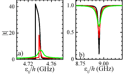
Figure 3: The normalized transmission amplitude as a function of the normalized magnetic flux $\varepsilon_{0}/h$. We obtain (a) an amplification and (b) an attenuation of the input signal. The transmission coefficient strongly depends on relaxations terms. Parameters for (a): $\Gamma_{1}/2\pi=4.8$, $6$, $8$ MHz and $\Gamma_{\phi}/2\pi=0.15$, $2.8$, $2$ MHz for black, red, and green curve,respectively; parameters for (b): $\Gamma_{1}/2\pi=0.8$, $4.8$, $6$ MHz and $\Gamma_{\phi}/2\pi=0.2$, $2$, $2.8$ MHz for black, red, and green curve, respectively.

Fig. 3 is plotted for the following parameters $\Delta/h=3.7$ GHz, $\mathrm{g}_{1}/2\pi$ $=0.8$ MHz, $\omega_{\mathrm{r}}/2\pi$ $=2.5$ GHz, $\omega_{\mathrm{d}}=3\omega_{\mathrm{r}},$ $\kappa/2\pi=30$ kHz, $\xi_{\mathrm{p}}=0.05\kappa$, $\omega_{p}=$ $\omega_{r}$, $A_{\text{d}}/h=7$ GHZ. The transmission coefficient sharp changes in the value at the magnetic flux about $\varepsilon_{0}/h=4.7$ GHz and $\varepsilon_{0}/h=8.9$ GHz. In the former case, the amplitude of the transmission signal increases. In the latter case, the transmission signal attenuates.

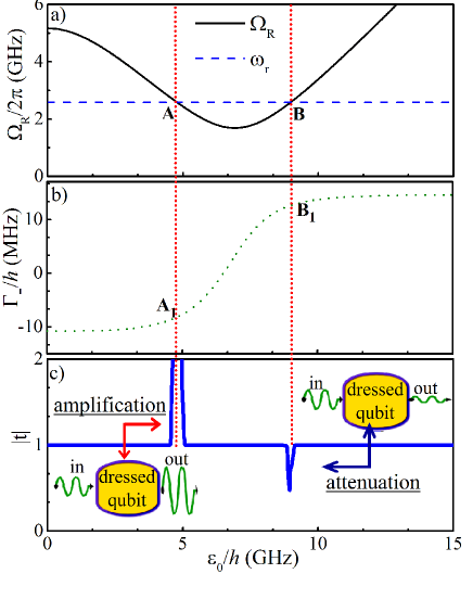
Figure 4: A schematic of the processes in the doubly-dressed system. (a) The black solid line is the Rabi frequency $\Omega_{\mathrm{R}}=\widetilde{\Delta E}/h$ of the dressed qubit. The blue dashed line is the resonator frequency $\omega_{\mathrm{r}}$. In the points of the intersection, denoted by A and B, the dressed system and the resonator exchange the energy. The dressed system influences on the passed signal. The output signal increases or decreases. The type of the process depends on the population of the energy states (see (b) and (c)). If the relaxation down $\widetilde{\Gamma}_{\downarrow}$ is smaller than the excitation $\widetilde{\Gamma}_{\uparrow}$, it will be an amplification of the transmitted signal ($\widetilde{\Gamma}_{-}<0$, point A₁). When the opposite situation is realized ($\widetilde{\Gamma}_{-}>0$), it will be an attenuation. (b) The difference between relaxations from level $|0\rangle$to level $|1\rangle$ and from level $|1\rangle$ to level $|0\rangle$. According to this graphics, we expect an inverse population in the system. (c) Transmission amplitude as a function of the magnetic flux $\varepsilon_{0}.$

The amplification of the signal takes place in the system when the Rabi frequency $\Omega_{\mathrm{R}}$ is close to the resonator frequency (see Fig. 4(a),(c)). We obtain the resonant exchange of energy between the probing signal and the dressed states. The direction of the energy transfer is specified by the difference between dissipative rates of the states (see Fig. 4(b)).

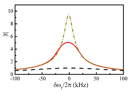
Figure 5: Normalized transmission amplitude as a function of the resonator detuning.  The dash-dot line and the solid line are plotted for $A_{\text{d}}/h=35$ $\mathrm{GHz}$, and the dash line is plotted for $A_{\text{d}}/h=0$. The parameters of the system are same as for Fig. 3. The relaxations rates are $\Gamma_{1}/2\pi=9$ MHz, $\Gamma_{\phi}/2\pi=4.8$ MHz. The dash-dot and dash lines are plotted for $T=0$ K, the solid line is plotted for $T=0.1$ K.

The analysis of Eqs. (19) and (21) demonstrates that we can considerably effect on it by varying of the relaxation coefficient and the amplitudes of the probing and driving signals. In Fig. 3 it is demonstrated how the variation of the relaxation coefficient effects on the amplification and the attenuation in the system. Such results were experimentally demonstrated in papers Oelsner13 ; Wu77 ; Khitrova88 ; Neilinger15 . The Fig. 6 is an example of the variation of the parameters.

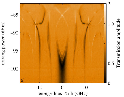
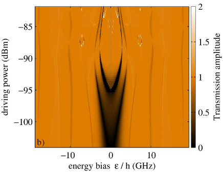
Figure 6: a) Measured normalized transmission amplitude of a probe signal applied at the fundamental mode frequency $\omega_{r}/2\pi=2.5$ GHz, while the qubit energy bias $\varepsilon$ and the driving amplitude $A_{\mathrm{d}}$ are varied. The latter is applied in the third harmonic of the resonator. The probing power takes a value of -$127$ dBm. b) Calculation results from (22). The calculation is carried out by splitting the bias axes in parts where the k-th. resonance is dominant but under consideration the energy level shift also induced by the neighboring resonances. The parameters of the qubit- resonator system, $\Delta\approx 3$ GHz, $\mathrm{g}_{1}/2\pi=4$ MHz, $\Gamma_{1}/2\pi=0.75$ MHz, $\Gamma_{\phi}/2\pi=30$ MHz, and $\kappa/2\pi=22$ kHz were defined by separate experiments

Consider Eqs. (19)-(21) at the resonance point ($\widetilde{\Delta E}=\omega_{\mathrm{p}}$) when the detuning of the resonator $\delta\omega_{\mathrm{r}}=0$. Then Eqs. (19) and (20) are simplified. We take into account that the average of the operator $\langle\tilde{\sigma}_{z}\rangle$ under weak probing signal is given by Eq. (23). For small deviations $\widetilde{\varepsilon}=$ $\Delta E-\hbar\omega_{d}$ the transmission amplitude is given by the following formula

$$\left|\,t\right|=\left|1-\frac{8\varepsilon_{0}^{2}\text{g}_{1}^{2}\widetilde{\varepsilon}}{\Delta E^{2}Q\widetilde{\Delta}\Gamma_{1}\kappa}\right|,$$ (28)

where $Q=\left((\bar{n}_{th}+\frac{1}{2})+\frac{\Gamma_{\phi}}{\Gamma_{1}}\right)\left(\left(2\bar{n}_{th}+\frac{3}{2}\right)+\frac{\Gamma_{\phi}}{\Gamma_{1}}\right).$

The Eq. (28) allows to roughly estimate effect of the system parameters on the transmission amplitude $t$ as a first approximation. The non-zero temperature leads to abatement of the amplification. The qubit relaxation $\Gamma_{1}$ and dephasing $\Gamma_{\phi}$ rates should be small, then we have system with long coherent time. We can use the asymptotic of the Bessel function in the limit of the high amplitudes of the driving signal $A_{\mathrm{d}}$:

$$\widetilde{\Delta}^{(k)}\propto\sqrt{\frac{k^{2}\omega_{\mathrm{d}}^{3}\Delta E}{A_{\mathrm{d}}\varepsilon_{0}^{3}}}\propto\frac{1}{\sqrt{A_{\mathrm{d}}}}.$$ (29)

The transmission coefficient $t$ is proportional to the square root of the driving amplitude $A_{\mathrm{d}}$ (see Eq. (28)). The increase of the driving photon number in the system by preference.

V Amplification with phase-slip qubit

We consider in this section the situation, where there is a so-called phase-slip qubit (PSQ) coupled to the transmission-line resonator. Our aim is to clarify similarities and distinctions from the previously considered case, where we had a flux qubit coupled to the resonator.

The coherent quantum phase slip has been discussed theoretically in Refs. Mooij05 ; Mooij06 and demonstrated experimentally in Ref. Astafiev12 . It describes a phenomenon exactly dual to the Josephson effect; whereas the latter is a coherent transfer of charges between superconducting leads, the former is a coherent transfer of vortices or fluxes across a superconducting wire. The similar behavior of the coherent quantum phase slip to Josephson junction allows to consider it as a part of the qubit-resonator system. The quantum phase slip process is characterized by the Josephson energy $E_{\mathrm{s}}$, which couples the flux states, resulting in the Hamiltonian, Ref. Mooij05 ; Mooij06 ,

$$H = -\frac{1}{2}E_{\mathrm{s}}\left(\left|N+1\right\rangle\left\langle N\right|+\left|N\right\rangle\left\langle N+1\right|\right)+$$

$$+E_{N}\left|N\right\rangle\left\langle N\right|,$$

which is dual to the Hamiltonian of a superconducting island connected to a reservoir through a Josephson junction; $N$ is the number of the fluxes in the narrow superconducting wire, $E_{N}=\left(\Phi_{\mathrm{ext}}-N\Phi_{0}\right)^{2}/2L_{k}$ is the state energy, $\Phi_{\mathrm{ext}}$ is an external magnetic flux, $L_{k}$ is the length of the nanowire. The ground and excited states can be related to the flux basis: $\left|g\right\rangle=\sin\frac{\alpha}{2}\left|N\right\rangle+\cos\frac{\alpha}{2}\left|N+1\right\rangle$ and $\left|e\right\rangle=\cos\frac{\alpha}{2}\left|N\right\rangle-\sin\frac{\alpha}{2}\left|N+1\right\rangle$, where the mixing angle is $\alpha=\arctan E_{\mathrm{s}}/\varepsilon_{0}$; the energy splitting between the ground and excited states is $\Delta E=\sqrt{\varepsilon_{0}^{2}+E_{\mathrm{s}}^{2}}$. In the rotating wave approximation, the effective Hamiltonian of the system resonantly driven by a classical microwave field with amplitude $\xi_{\mathrm{d}}\cos\left(\Delta E/\hslash\right)$ is $H_{\mathrm{RWA}}=\frac{\hslash\Omega}{2}\sigma_{z}.$ Such Hamiltonian coincides with the Hamiltonian of the flux qubit in the RWA up to the notations Wendin . The interaction between the PSQ and the two-mode resonator can be described by Hamiltonian (II). We demonstrate the transmission coefficient for a real experimental PSQ in Fig. (7). We use data which corresponds to Ref. Astafiev12 . Equations (19)-(21) are also applicable for the PSQ-resonator system. The doubly-dressed approach is useful instrument for description of the quantum behavior of the different mesoscopic systems.

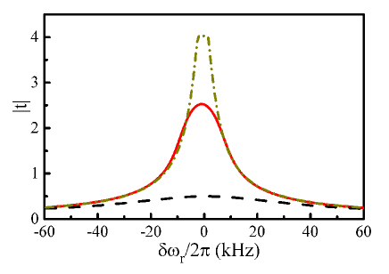
Figure 7: The transmission amplitude for PSQ-resonator system at the value of the driving amplitude, corresponding to the maximal amplification. The dash-dot line and the solid line are plotted for $A_{\text{d}}/h=35$ $\mathrm{GHz}$, and the dash line is plotted for $A_{\text{d}}/h=0$ . Parameters for the calculations are the following: $\Delta E/h=$ 4.9 GHz, $\omega_{\text{r}}/2\pi=2.4$ GHZ, $\kappa/2\pi=$ 30 kHz. Note that the half-width at half-maximum of the transmission line decreases under pumping. The dash-dot and dash lines is plotted for $T=0$ K, the solid line is plotted for $T=0.1$ K.

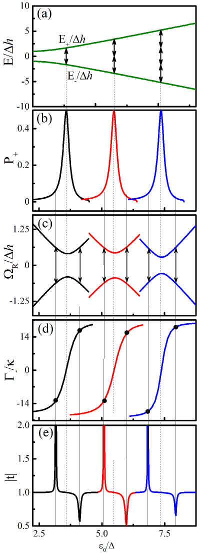
Figure 8: We consider the processes taking place in the qubit-resonator system. (a) The energy level of the qubit. The one, two and three photon resonances are marked by the arrows. (b) The maximum value of the excited state probability of the dressed qubit corresponds to the resonance condition $\widetilde{\Delta E}=n\hbar\omega_{\mathrm{p}}$ for integer $n$. (c) The qubit interaction with driving high-amplitude signal leads to a renormalization of the energy levels of the qubit. (d) The inverse population is typical for the system with various relaxation times between the dressed levels. (e) It corresponds to the energy transfer from the dressed states in the probe signal. When the opposite situation is realized, the amplitude of the probe signal reduces.

VI Conclusions

We studied the evolution of the doubly-driven qubit-resonator system. We demonstrated the possibility of a large amplification of the input signal and the ability of almost full reflection of the probe signal in the system. The value of the transmitted signal depends on all the system parameters, of which the coupling coefficient g₁ and the relaxation rates $\kappa$ and $\Gamma_{1,\phi}$ are the most influential. The numerical simulation of the different qubit-resonator system from real experimental papers allows to estimate the optimal parameters for this samples. In particular, we have found that for both amplification and attenuation the following parameter values are optimal: g$/\Delta\sim 10^{-4}-10^{-2}$, $\kappa\lesssim\xi_{p}$, $\Gamma_{1}/\Delta\sim 10^{-2}-10^{-1}$, and $\Gamma_{\phi}/\Delta\sim 10^{-2}-10^{-1}$. The temperature noise (non-zero temperature) is diminished the transmission amplitude.

References

• (1) A.N. Omelyanchouk, E.V. Il’ichev, S.N. Shevchenko, Quantum coherent phenomena in Josephson qubits (in Russian), Naukova Dumka, Kiev, 2013.
• (2) G. Wendin and V.S. Shumeiko, Low Temp. Phys. 33, 9 (2007).
• (3) Ya. S. Greenberg, E. Il ichev Phys. Rev. B 77 , 094513 (2008).
• (4) G. Oelsner, S.H.W. van der Ploeg, P. Macha, U. Hübner, D. Born, E. Il’ichev, H.-G. Meyer, M. Grajcar, S. Wünsch, M. Siegel, A. N. Omelyanchouk, and O. Astafiev, Phys. Rev. B 81, 172505 (2010).
• (5) S. Ashhab, J.R. Johansson, A.M. Zagoskin, and F. Nori, New J. Phys. 11, 023030 (2009).
• (6) H. Wang, H.-C. Sun, J. Zhang, and Y. Liu, Sc. Ch. Phys., 55(12), 2264 (2014).
• (7) C. Andersen, G. Oelsner, E. Il’ichev, and K.Molmer, Phys. Rev. A 89, 033853 (2014).
• (8) S.N. Shevchenko, G. Oelsner, Ya.S. Greenberg, P. Macha, D.S. Karpov, M. Grajcar, A.N. Omelyanchouk, and E. Il’ichev, Phys. Rev. B 84, 184504 (2014).
• (9) A.P. Sajko, G.G. Fedoruk, and S.A. Markevich, JETP Letters 101, 3 (2014).
• (10) A.P. Saiko, R. Fedaruk, and S.A. Markevich, J. Phys. B: At. Mol. Opt. Phys. 47, 155502 (2014).
• (11) A.P. Saiko, R. Fedaruk, and S.A. Markevich, J. Exp. Theor. Phys. 118, 655 (2014).
• (12) C. Xu, A. Poudel, and M.G. Vavilov, Phys. Rev. A 89, 052102 (2014).
• (13) J. Hauss, A. Fedorov, S. André, V. Brosco, C. Hutter, R. Kothari, S. Yeshwant, A. Shnirman, and G. Schön, New Journal of Physics 10, 095018 (2008).
• (14) G. Oelsner, P. Macha, O. V. Astafiev, E. Il’ichev, M. Grajcar, U. Hübner, B. I. Ivanov, P. Neilinger, and H.-G. Meyer, Phys. Rev. Lett 110, 053602 (2013).
• (15) F. Forster, M. Muhlbacher, R. Blattmann, D. Schuh, W. Wegscheider, S. Ludwig, and S. Kohler, arXiv:1510.01976.
• (16) J. Hauss, A. Fedorov, C. Hutter, A. Shnirman, and G. Schön, Phys. Rev. Lett. 100 , 037003 (2010).
• (17) A.M. Satanin, M.V. Denisenko, A.I. Gelman, and F. Nori, Phys. Rev. B 90, 104516 (2014).
• (18) Ya. S. Greenberg, Phys. Rev. B 76, 104520 (2007).
• (19) N. Bergeal, F. Schackert, M. Metcalfe, R. Vijay, V.E. Manucharyan, L. Frunzio, D.E. Prober, R.J. Schoelkopf, S.M. Girvin, and M.H. Devoret, Nature 465, 64 (2010).
• (20) B. Abdo, K. Sliwa, S. Shankar, M. Hatridge, L. Frunzio, R. Schoelkopf, and M. Devoret, Phys. Rev. Let. 112, 167701 (2014).
• (21) O. Astafiev, A. A. Abdumalikov Jr., A. M. Zagoskin, Yu. A. Pashkin, Y. Nakamura, and J. S. Tsai, Phys. Rev. Lett. 112, 068103 (2010).
• (22) Z.R. Lin, K. Inomata, W.D. Oliver, K. Koshino, Y. Nakamura, J.S. Tsai, and T. Yamamoto, Appl. Phys. Lett. 103, 132602 (2013).
• (23) J. E. Mooij and Yu. V. Nazarov, Nature Phys. 2, 169 (2006).
• (24) O. V. Astafiev, L. B. Ioffe, S. Kafanov, Yu. A. Pashkin, K. Yu. Arutyunov, D. Shahar, O. Cohen, and J. S. Tsai, Nature 484, 355 (2012).
• (25) M.O. Scully and M.S. Zubairy, Quantum Optics, Cambridge (1997).
• (26) L.S. Bishop, J.M. Chow, J. Koch, A.A. Houck, M.H. Devoret, E.Thuneberg, S.M. Girvin, and R. J. Schoelkopf, Nature Phys. 5,105 (2009).
• (27) K. Koshino, H. Terai, K. Inomata, T. Yamamoto, W. Qiu, Z. Wang, and Y. Nakamura, Phys. Rev. Lett. 110, 263601 (2013).
• (28) F.Y. Wu , S. Ezekiel, M. Ducloy, and B. R. Mollow, Phys. Rev. Lett. 38, 1077 (1977).
• (29) G. Khitrova and J.F. Valley, Phys. Rev. Lett. 60, 1126 (1988).
• (30) P. Neilinger, M. Rehák, M. Grajcar, G. Oelsner, U. Hübner, E. Il’ichev, Phys. Rev. B 91, 104516 (2015).
• (31) D.M. Pozar, Microwave Engineering, Wiley, New York, 3rd ed., (1990).
• (32) E.A. Temchenko, S.N. Shevchenko, and A.N. Omelyanchouk Phys. Rev. B 83, 144507 (2011).
• (33) J. Hwang, M. Pototschnig, R. Lettow, G. Zumofen, A. Renn, S. Gĕotzinger, and V. Sandoghdar, Nature 460, 76 (2009).
• (34) I. Gerhardt, G. Wrigge, P. Bushev, G. Zumofen, M. Agio, R. Pfab, and V. Sandoghdar, Phys. Rev. Lett. 98, 033601 (2007).
• (35) G. Wrigge, I. Gerhardt, J. Hwang, G. Zumofen, and V. Sandoghdar, Nature Physics 4, 60 (2008).
• (36) E. Il’ichev, A.Yu. Smirnov, M. Grajcar, A. Izmalkov, D. Born, N. Oukhanski, Th. Wagner, W. Krech, H.-G. Meyer, and A.M. Zagoskin, Low Temp. Phys. 30, 620 (2004).
• (37) S.N. Shevchenko, A.N. Omelyanchouk, and E. Il’ichev, Low Temp. Phys. 38, 283 (2012).
• (38) S. André, Pei-Qing Jin, V. Brosco, J. Cole, A. Romito, A. Shnirman, and G. Schön, Phys. Rev. A 82, 053802 (2010).
• (39) A.N. Omelyanchouk, S.N. Shevchenko, Ya.S. Greenberg, O. Astafiev, and E. Il’ichev, Low Temp. Phys. 36, 893 (2010).
• (40) P. Neilinger, J. Bogar, S. N. Shevchenko, G. Oelsner, D. S. Karpov, O. Astafiev, M. Grajcar, and E. Il’ichev, in preparation.
• (41) J. E. Mooij and C. J. Harmans, New J. Phys. 7, 219 (2005).