Rotational dynamics of a diatomic molecular ion in a Paul trap

Abstract

We present models for a heteronuclear diatomic molecular ion in a linear Paul trap in a rigid-rotor approximation, one purely classical, the other where the center-of-mass motion is treated classically while rotational motion is quantized. We study the rotational dynamics and their influence on the motion of the center-of-mass, in the presence of the coupling between the permanent dipole moment of the ion and the trapping electric field. We show that the presence of the permanent dipole moment affects the trajectory of the ion, and that it departs from the Mathieu equation solution found for atomic ions. For the case of quantum rotations, we also evidence the effect of the above-mentioned coupling on the rotational states of the ion.

I Introduction

Laser-cooled or sympathetically-cooled atomic and molecular ions have been in the spotlight in recent years, due to their great potential in the study and development of many fields, such as chemical reactions,Mølhave and Drewsen (2000); Blythe et al. (2005); Baba and Waki (2002); Tong et al. (2012); Chang et al. (2013); Rösch et al. (2014) high-precision spectroscopy,Douglas, Frank, and Mao (2005); Leanhardt et al. (2011); Loh et al. (2013) atomic optics, and in many other fast developing fields related to quantum information and quantum computing, where the manipulation of the internal states of these ions has become possible.Weidinger and Gruebele (2008); Buluta et al. (2008); Alonso et al. (2013); Amniat-Talab, Saadati-Niari, and Guérin (2012); Leibfried (2012); Shi et al. (2013)

One of the most applied techniques to trap these cold ions is known as the Paul trap, using time-dependent radio-frequency electric fields.Paul (1990) Paul traps, specifically those with a linear configuration,Prestage, Dick, and Maleki (1989) consist of electrodes designed to surround an inner space where the trapping of a single charged particle, as well as the simultaneous trapping a string of charged particles, occurs. This makes them highly suitable to be used in experiments involving laser control of the ions, since the spacing between the electrodes as well as the spacing between the ions provide a good environment for this purpose.Raizen et al. (1992a, b); Brkić et al. (2006) In this regard, large scale studies of trapped ions in large scales, in the form of Coulomb crystals, have become feasible, with promising developments for large-scale quantum simulations and quantum computations.Buluta et al. (2008); Drewsen et al. (2003); Porras and Cirac (2006); Willitsch (2012)

While there have been many experimental studies using molecular ions, on the theoretical side there have been few attempts to treat them differently than atomic ions, at least with respect to their interaction with the trapping electric field. In particular, the rotation of the molecular ions has been considered mostly with respect to a coupling with an external laser field.Vogelius, Madsen, and Drewsen (2006); Lazarou, Keller, and Garraway (2010); Shi et al. (2013); Berglund, Drewsen, and Koch (2015)

In this paper we study the dynamical behavior of a rigid, heteronuclear diatomic molecular ion trapped inside a linear Paul trap. We investigate the coupling of the permanent dipole moment of the molecular ion with the trapping electric field and its effect on the rotational dynamics of the ion and also on the center-of-mass motion of the ion. We develop classical and semi-classical models of the molecular ion, where rotation is treated classically and quantum mechanically, respectively. We carry out simulations of the motion of the center of mass, including the effects of the interaction between the trapping electric field and the permanent dipole moment of the molecular ion, by solving the classical equations of motion. Classical rotation is treated using the “body vector method,”Evans (1977) while a basis set of spherical harmonics is used to describe the quantum rotational wave function.

This paper is organised as follows. First, we introduce our model for a rigid diatomic molecular ion trapped inside a linear Paul trap (Sec. II). The numerical methods for the classical and semi-classical simulations are described in Sec. III. The results obtained from both classical and semi-classical methods are presented in Sec. IV.1 and Sec. IV.2, respectively. Finally, concluding remarks are given in Sec. V.

II Hamiltonian of a rigid diatomic molecular ion in a linear Paul trap

II.1 Quantum-mechanical Hamiltonian

We consider a diatomic molecular ion inside a linear Paul trap,Prestage, Dick, and Maleki (1989); Major, Gheorghe, and Werth (2005) combining a quadrupole, time-dependent, radio-frequency electric potential and a static electric potential,

$$\Phi(t)=\Phi_{\mathrm{rf}}(t)+\Phi_{\mathrm{s}}\,,$$ (1)

in which, for an ion located at position $(X,Y,Z)$,

$$\Phi_{\mathrm{rf}}(t) =\frac{1}{2}\frac{V_{0}}{r_{0}^{2}}\left(X^{2}-Y^{2}\right)\cos\Omega t\,,$$ (2a)

$$\Phi_{\mathrm{s}} =\frac{\kappa U_{0}}{z_{0}^{2}}\left[Z^{2}-\frac{1}{2}\left(X^{2}+Y^{2}\right)\right]\,,$$ (2b)

where $V_{0}$ and $U_{0}$ are the amplitudes of the radio-frequency (with frequency $\Omega$) and static potentials, respectively, $r_{0}$ and $z_{0}$ are parameters representing the dimensions of the trap, and $\kappa$ is the geometric factor, which is solely dependent on the configuration of the trap.Raizen et al. (1992a)

The Hamiltonian of a free diatomic molecular ion in a rigid rotor model, where the nuclear vibrations of the ion are ignored, has the form

$$\hat{H}=-\frac{\hbar^{2}}{2M}\nabla^{2}_{\mathbf{R}}+\frac{B\hat{J}^{2}}{\hbar^{2}}\,,$$ (3)

with $M$ the total mass of the diatomic molecular ion. The derivatives in the first term are with respect to the position of the center of the mass of the ion, $\mathbf{R}$. The second term represents the rotational energy of the ion, with $\hat{J}$ the total angular momentum operator, the operator $\hat{J}^{2}$ having eigenvalues $J(J+1)\hbar^{2}$, and the rotational constant is

$$B=\frac{\hbar^{2}}{2I},$$ (4)

where $I=m_{\mathrm{red}}r^{2}$ is the moment of inertia, with $m_{\mathrm{red}}$ and $r$ the reduced mass and internuclear distance, respectively. The rigid rotor approximation we are using implies that the latter is fixed, i.e., $r=\mathrm{const.}$

In addition to having a non-zero electric charge, we take the diatomic molecular ion to be heteronuclear, which means that it possesses a permanent dipole moment that will also interact with the electric field of the Paul trap. Adding the interaction of the ion with the trapping field to Hamiltonian (3), we get

$$\hat{H}=-\frac{\hbar^{2}}{2M}\nabla^{2}_{\mathbf{R}}+\frac{B\hat{J}^{2}}{\hbar^{2}}+Ze\Phi(\mathbf{R},t)-\bm{\mu}\cdot\mathbf{E}(\mathbf{R},t)\,,$$ (5)

in which $Ze$ is the total charge of the ion (with $e$ the elementary charge), $\bm{\mu}$ is the permanent dipole moment, of magnitude $\mu_{0}$, and $\mathbf{E}\equiv-\nabla\Phi$ is the trapping electric field, at the position $\mathbf{R}$ of the ion.

II.2 Classical Hamiltonian

Classically, we approximate the diatomic molecular ion inside a trapping potential as a dipolar rigid rotor, consisting of two masses $m_{-}$ and $m_{+}$ with partial charges $\delta_{-}$ and $\delta_{+}$, respectively, kept spatially separated at a constant distance. A complete derivation of the kinetic and potential energy terms is given in Appendix A, resulting in the classical Hamiltonian

$$H=K+V=\frac{1}{2}M\dot{\mathbf{R}}^{2}+\frac{1}{2}I\dot{\bm{\omega}}^{2}+Ze\Phi(\mathbf{R},t)-\bm{\mu}\cdot\mathbf{E}(\mathbf{R},t)\,,$$ (6)

in the point-dipole approximation, with $I$ the moment of inertia and $\dot{\bm{\omega}}$ the angular velocity. The corresponding classical equation of motion for the center of mass is

$$M\mathbf{\ddot{R}}+Ze\bm{\nabla}\Phi(\mathbf{R},t)-\bm{\nabla}\left[\bm{\mu}\cdot\mathbf{E}(\mathbf{R},t)\right]=0\,,$$ (7)

which differs from that of a classical atomic ionGhosh (1995); Major, Gheorghe, and Werth (2005); Hashemloo, Dion, and Rahali (2016) in an additional term representing the coupling of the electric field with the permanent dipole moment. As shown in many previous works, the equations of motion of an atomic ion inside a Paul trap obey the Mathieu equationGhosh (1995); Major, Gheorghe, and Werth (2005)

$$\frac{\rm d^{2}\mathbf{R}}{\rm d\tau^{2}}+(a-2q\cos 2\tau)\mathbf{R}=0\,.$$ (8)

The Mathieu equation has stable solutions and hence bounded trajectories depending on whether its parameters ($a$ and $q$) fall within a certain range – called stability regions – in the $a-q$ plane or not.Wolf (2010) For an ion inside a Paul trap, $a$ and $q$ depend on the mass of the ion, the magnitude of the field, and the parameters of the trap. For an ion in a linear Paul trap, corresponding to the potential in Eqs. (1) and (2), setting $\tau=\Omega t/2$, we have

$$a_{x}=a_{y} =-\frac{4Ze}{M\Omega^{2}}\frac{\kappa U_{0}}{z_{0}^{2}},$$ (9a)

$$a_{z} =\frac{8Ze}{M\Omega^{2}}\frac{\kappa U_{0}}{z_{0}^{2}},$$ (9b)

$$q_{x}=-q_{y} =-\frac{2Ze}{M\Omega^{2}}\frac{V_{0}}{r_{0}^{2}},$$ (9c)

$$q_{z} =0\,.$$ (9d)

Even though the equation of motion for a diatomic molecular ion, Eq. (7), does not reduce to a Mathieu equation, taking the term $\bm{\nabla}\left[\bm{\mu}\cdot\mathbf{E}(\mathbf{R},t)\right]$ as a small perturbation (we will investigate this below), one can still use the stability criteria of the Mathieu equation as a guideline for the stability of the trap for a molecular ion.

III Numerical methods

III.1 Classical approach

The classical representation of the rigid rotor, Hamiltonian (6), has five degrees of freedom: the three Cartesian coordinates of the center of mass, along with two angles positioning the internuclear axis of the diatomic ion in space, see Fig. 1.

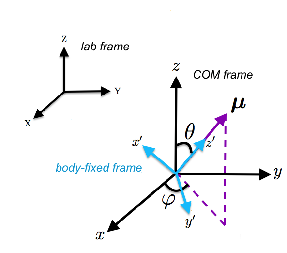
Figure 1: (Color online) The orientation of the permanent dipole moment $\bm{\mu}$ of a diatomic molecule in space with respect to the center-of-mass (COM) frame $(x,y,z)$, which is indicated by angles $\varphi$ and $\theta$. The body-fixed frame $({x}^{\prime},{y}^{\prime},{z}^{\prime})$ shows the principal axes (or symmetry axes) of this molecule. The orientation of the dipole moment is fixed along ${z}^{\prime}$. The COM frame is aligned with the laboratory frame $(X,Y,Z)$, but has its origin at the center-of-mass of the molecule.

We consider three different coordinate systems: the laboratory-fixed system $(X,Y,Z)$, the COM (center-of-mass) system $(x,y,z)$, which is taken to be parallel to the laboratory-fixed frame, but centered on the center of mass of the molecular ion (see also Appendix A), and the body-fixed system $({x}^{\prime},{y}^{\prime},{z}^{\prime})$, with its origin at the center of mass, but with axis ${z}^{\prime}$ always co-linear with the internuclear axis (and hence with the dipole moment $\bm{\mu}$).

Expanding the dipole moment vector into its components in the COM frame $(x,y,z)$, we get

$$\bm{\mu}=\mu_{0}[\sin\theta\cos\varphi\mathbf{\hat{x}}+\sin\theta\sin\varphi\mathbf{\hat{y}}+\cos\theta\mathbf{\hat{z}}]\,,$$ (10)

in which $\mu_{0}$ is the magnitude of the dipole moment and $\mathbf{\hat{x}}$, $\mathbf{\hat{y}}$, and $\mathbf{\hat{z}}$ are unit vectors along the axes and $\theta$ and $\varphi$ are the polar and azimuthal angles, respectively (see Fig. 1). We can also expand the trapping electric field at the position of the ion into its component as

$$\mathbf{E}(\mathbf{R},t)=-\nabla\Phi(\mathbf{R},t)=\left[\frac{\kappa U_{0}}{z_{0}^{2}}-\frac{V_{0}}{r^{2}_{0}}\cos\Omega t\right]X\mathbf{\hat{x}}+\left[\frac{\kappa U_{0}}{z_{0}^{2}}+\frac{V_{0}}{r^{2}_{0}}\cos\Omega t\right]Y\mathbf{\hat{y}}-\frac{2\kappa U_{0}}{z^{2}_{0}}Z\mathbf{\hat{z}}\,,$$ (11)

where we have used the potential defined by Eqs. (1) and (2). The coupling term of Eq. (6) then has the form

$$\bm{\mu}\cdot\mathbf{E} =\left[\frac{\kappa U_{0}\mu_{0}\sin\theta\cos\varphi}{z_{0}^{2}}-\frac{V_{0}\mu_{0}\sin\theta\cos\varphi}{r^{2}_{0}}\cos\Omega t\right]X$$

$$\quad+\left[\frac{\kappa U_{0}\mu_{0}\sin\theta\sin\varphi}{z_{0}^{2}}+\frac{V_{0}\mu_{0}\sin\theta\sin\varphi}{r^{2}_{0}}\cos\Omega t\right]Y$$ (12)

$$\quad-\left[\frac{2\kappa U_{0}\mu_{0}}{z^{2}_{0}}\cos\theta\right]Z\,.$$

It is clearly evident from this equation that the interaction between the dipole moment and the electric field has not only a spatial dependence, but also is dependent on the orientation of the ion inside the trap.

A direct numerical simulation of the equations of motion corresponding to the Hamiltonian (6) is impractical, as these equations contain a term in $1/\sin^{2}\theta$, and thus are singular at $\theta=0$. In order to avoid this problem, we use the “body vector method,”Evans (1977) where it is assumed that the diatomic molecular ion is actually a rigid rotor (di-axes body) with a principal inertia tensor of the formEvans (1977)

$$I=\begin{pmatrix}I_{x^{\prime}}&0&0\\ 0&I_{y^{\prime}}&0\\ 0&0&0\end{pmatrix}\,$$ (13)

in which $I_{x^{\prime}}=I_{y^{\prime}}=I\equiv m_{\mathrm{red}}r^{2}$ ($m_{\mathrm{red}}$ is the reduced mass and $r$ is the internuclear distance) and $I_{z^{\prime}}=0$ (i.e., there is no rotation around the internuclear axis), all expressed in the body-fixed coordinate system $(x^{\prime},y^{\prime},z^{\prime})$. Following the body vector method, we introduce unit vectors along these axes, namely $\mathbf{\hat{x}}^{\prime}$, $\mathbf{\hat{y}}^{\prime}$, $\mathbf{\hat{z}}^{\prime}$. These unit vectors have components with respect to the COM-frame

$$\mathbf{\hat{u}}^{\prime}=({u}^{\prime}_{x},{u}^{\prime}_{y},{u}^{\prime}_{z})\,.$$ (14)

where $\mathbf{\hat{u}}^{\prime}\in\left\{\mathbf{\hat{x}}^{\prime},\mathbf{\hat{y}}^{\prime},\mathbf{\hat{z}}^{\prime}\right\}$.

Setting the internuclear axis (or $\bm{\mu}$) along the $z^{\prime}$ axis, the unit vector $\mathbf{\hat{z}}^{\prime}$ simply gives the direction of the dipole moment in space.Evans (1977) These vector are similar to the variables described by CheungCheung and Powles (1975); Cheung (1976) to avoid singularities in the equations of motion for diatomic molecules. As a result, we can write the dipole moment vector as

$$\bm{\mu}=\mu_{0}\mathbf{\hat{z}}^{\prime}\,,$$ (15)

in which the components of $\mathbf{\hat{z}}^{\prime}$ can be written in terms of $\theta$ and $\varphi$

$${z}^{\prime}_{x} =\sin\theta\cos\varphi\,,$$

$${z}^{\prime}_{y} =\sin\theta\sin\varphi\,,$$ (16)

$${z}^{\prime}_{z} =\cos\theta\,,$$

in accord with Eq. (14) and Fig. 1.

We can now simply rewrite Eq. (III.1) using the new representation of the dipole moment, with the interaction term in the Hamiltonian not being explicitly dependent on the angles $(\theta,\varphi)$. Instead, the change in the direction of the dipole moment is equivalent to the temporal change of the direction of the principal axes according to

$$\hat{\dot{\mathbf{u}}}^{\prime}=\bm{\omega}_{P}\times\mathbf{\hat{u}}^{\prime}\,,$$ (17)

where $\bm{\omega}_{P}$ is the principal angular velocity of the dipole, precessing around its principal rotational axes. To write the equations of motion, we need to calculate the torque in the lab-fixed frame, $\mathbf{T}_{L}=\bm{\mu}\times\mathbf{E}$, which is imposed on the dipole moment by the external electric field.Evans and Murad (1977) To calculate the time evolution of the dipole moment, Eq. (17), we need the principal torque $\mathbf{T}_{P}$, which is obtained from the relationEvans (1977)

$$\mathbf{T}_{L}=\mathbf{A}^{T}\mathbf{T}_{P}\,,$$ (18)

where $\mathbf{A}^{T}$ is the transpose of the rotation matrixGoldstein, Poole, and Safko (2002) whose columns are the principal axes unit vectorsEvans (1977)

$$\mathbf{A}^{T}=(\mathbf{\hat{x}}^{\prime},\mathbf{\hat{y}}^{\prime},\mathbf{\hat{z}}^{\prime})\equiv\begin{pmatrix}x^{\prime}_{x}&y^{\prime}_{x}&z^{\prime}_{x}\\ x^{\prime}_{y}&y^{\prime}_{y}&z^{\prime}_{y}\\ x^{\prime}_{z}&y^{\prime}_{z}&z^{\prime}_{z}\end{pmatrix}\,.$$ (19)

As there is no rotation along the internuclear axis, $\omega_{Pz^{\prime}}=0$ and there is no torque in the $z_{P}$ direction [see Eq. (15)], $T_{Pz^{\prime}}=0$, the equations of motion for rotation are written as

$$I_{x^{\prime}}\dot{\omega}_{Px^{\prime}} =T_{Px^{\prime}}+\omega_{Py^{\prime}}\omega_{Pz^{\prime}}(I_{y^{\prime}}-I_{z^{\prime}})=T_{Px^{\prime}}$$

$$I_{y^{\prime}}\dot{\omega}_{Py^{\prime}} =T_{Py^{\prime}}+\omega_{Pz^{\prime}}\omega_{Px^{\prime}}(I_{z^{\prime}}-I_{x^{\prime}})=T_{Py^{\prime}}$$ (20)

$$I_{z^{\prime}}\dot{\omega}_{Pz^{\prime}} =0\,.$$

Finally, the equations which describe the dynamical behavior of the ion inside the linear Paul trap, classically, are

$$\frac{d\mathbf{R}}{dt} =\frac{\mathbf{P}}{M}\,,$$ (21a)

$$\frac{dP_{X}}{dt} =e\left[b_{1}-b_{2}\cos\Omega t\right]X+\mu_{0}\left[b_{1}-b_{2}\cos\Omega t\right]z^{\prime}_{x}\,,$$ (21b)

$$\frac{dP_{Y}}{dt} =e\left[b_{1}+b_{2}\cos\Omega t\right]Y+\mu_{0}\left[b_{1}+b_{2}\cos\Omega t\right]z^{\prime}_{y}\,,$$ (21c)

$$\frac{dP_{Z}}{dt} =-2eb_{1}Z-2\mu_{0}b_{1}z^{\prime}_{z}\,,$$ (21d)

$$\frac{d{\mathbf{\hat{u}}}^{\prime}}{dt} =\bm{\omega}_{P}\cdot{\mathbf{\hat{u}}}^{\prime}\,,\text{ where }\mathbf{\hat{u}}^{\prime}\in\left\{\mathbf{\hat{x}}^{\prime},\mathbf{\hat{z}}^{\prime}\right\}$$ (21e)

(since only two coordinates are necessary to locate the dipole in space, we obtain $$\mathbf{\hat{y}}^{\prime} \mathbf{\hat{y}}^{\prime}=\mathbf{\hat{z}}^{\prime}\times\mathbf{\hat{x}}^{\prime}$$ from ),

$$\frac{d\bm{\omega}_{P}}{dt} =\frac{1}{I}\mathbf{T}_{P}\ =\frac{1}{I}({\mathbf{A}^{\mathrm{T}}})^{-1}\mathbf{T}_{L}\,,$$ (21f)

with

$$T_{Lx} =\mu_{0}\left[-2b_{1}Zz^{\prime}_{y}-(b_{1}+b_{2}\cos\Omega t)Yz^{\prime}_{z}\right]\,,$$ (22a)

$$T_{Ly} =\mu_{0}\left[2b_{1}Zz^{\prime}_{x}+(b_{1}-b_{2}\cos\Omega t)Xz^{\prime}_{z}\right]\,,$$ (22b)

$$T_{Lz} =\mu_{0}\left[(b_{1}+b_{2}\cos\Omega t)Yz^{\prime}_{x}-(b_{1}-b_{2}\cos\Omega t)Xz^{\prime}_{y}\right]\,,$$ (22c)

where we have defined

$$b_{1}\equiv\frac{\kappa U_{0}}{z_{0}^{2}}\,,\quad b_{2}\equiv\frac{V_{0}}{r_{0}^{2}}\,.$$ (23)

III.2 Semi-classical approach

A direct simulation using the full quantum Hamiltonian (5) would be quite numerically intensive, owing to the five degrees of freedom, the large amplitude of the motion in the trap, and the impossibility of separating the problem along Cartesian coordinates (in contrast to the case for atomic ionsHashemloo, Dion, and Rahali (2016)) due to the coupling of the rotation with the trapping potential. Using the fact that the expectation value for the center-of-mass motion follows the classical equations of motion,Combescure (1986); Brown (1991); Glauber (1992); Hashemloo, Dion, and Rahali (2016) we instead build a semi-classical model, where the center-of-mass motion is treated classically, but the fully-quantum rotational wave function is calculated, according to the Schrödinger equation

$$i\hbar\frac{d}{dt}\Psi^{\mathrm{rot}}(\theta,\varphi;t)=\left[\frac{B}{\hbar}\hat{J}^{2}-\bm{\mu}\cdot\mathbf{E}(\mathbf{R},t)\right]\Psi^{\mathrm{rot}}(\theta,\varphi;t)\,,$$ (24)

where $\Psi^{\mathrm{rot}}(\theta,\varphi;t)$ is the rotational wave function of the molecular ion and $\mathbf{E}(\mathbf{R},t)$ is the trapping electric field at the position of the ion, $\mathbf{R}$, obtained classically, see Eqs. (33) below.

The wave function can be expanded on the basis of field-free rotor states (spherical harmonics) $Y_{J,M}(\theta,\varphi)$ as

$$\Psi^{\mathrm{rot}}(\theta,\varphi;t)=\sum_{J,M}D_{J,M}(t)Y_{J,M}(\theta,\varphi)\,,$$ (25)

where the expansion coefficients $D_{J,M}$ are time dependent complex values that determine the rotational state of the ion.

Solving the time-dependent Schrödinger equation (24) using the expression of the rotational wave function in Eq. (25),

$$i\hbar\sum_{J,M}\dot{D}_{J,M}(t)=\sum_{J,M}D_{J,M}(t)BJ(J+1)-\sum_{J,M}\sum_{{J}^{\prime},{M}^{\prime}}D_{{J}^{\prime},{M}^{\prime}}(t)\braket{J,M}{\bm{\mu}\cdot\mathbf{E}}{{J}^{\prime},{M}^{\prime}}\,,$$ (26)

results in a set of coupled equations for the time evolution of the coefficients,

$$\dot{D}_{J,M}(t)=-\frac{i}{\hbar}D_{J,M}(t)BJ(J+1)+\frac{i}{\hbar}\sum_{{J}^{\prime},{M}^{\prime}}D_{{J}^{\prime},{M}^{\prime}}(t)\braket{J,M}{\bm{\mu}\cdot\mathbf{E}}{{J}^{\prime},{M}^{\prime}}\,,$$ (27)

in which the kets $\ket{J,M}$ correspond to the spherical harmonics $Y_{J,M}(\theta,\varphi)$. Using Eq. (III.1) for the interaction of the dipole moment with the electric field and substituting trigonometric functions with their equivalent spherical harmonicsVarshalovich, Moskalev, and Khersonskiĭ (1988) gives

$$\bm{\mu}\cdot\mathbf{E}=\sqrt{\frac{2\pi}{3}}\mu_{0}\left[(E_{x}+iE_{y})Y_{1,-1}+\sqrt{2}E_{z}Y_{1,0}+(-E_{x}+iE_{y})Y_{1,1}\right]$$ (28)

and hence

$$\braket{J,M}{\bm{\mu}\cdot\mathbf{E}}{{J}^{\prime},{M}^{\prime}} =\sqrt{\frac{2\pi}{3}}\mu_{0}\left[\left(E_{x}+iE_{y}\right)\braket{J,M}{Y_{1,-1}}{{J}^{\prime},{M}^{\prime}}+\sqrt{2}E_{z}\braket{J,M}{Y_{1,0}}{{J}^{\prime},{M}^{\prime}}\right.$$

$$\quad\left.+\left(-E_{x}+iE_{y}\right)\braket{J,M}{Y_{1,1}}{{J}^{\prime},{M}^{\prime}}\right]\,,$$ (29)

Using Clebsch-Gordan coefficients and their related 3j-symbols, we haveVarshalovich, Moskalev, and Khersonskiĭ (1988)

$$\braket{J,M}{Y_{1,n}}{{J}^{\prime},{M}^{\prime}} =\int_{0}^{\pi}\int_{0}^{2\pi}Y^{*}_{J,M}(\theta,\varphi)Y_{1,n}(\theta,\varphi)Y_{{J}^{\prime},{M}^{\prime}}(\theta,\varphi)\sin\theta d\theta d\varphi$$

$$=(-1)^{n}\sqrt{\left[\frac{(2J+1)(3)(2{J}^{\prime}+1)}{4\pi}\right]}\begin{pmatrix}J&1&{J}^{\prime}\\ 0&0&0\end{pmatrix}\begin{pmatrix}J&1&{J}^{\prime}\\ -M&n&{M}^{\prime}\end{pmatrix}$$

$$=\sqrt{\left[\frac{(2{J}^{\prime}+1)(3)}{4\pi(2J+1)}\right]}C^{J0}_{{J}^{\prime}010}C^{JM}_{{J}^{\prime}{M}^{\prime}1n}\,,$$ (30)

with $n=-1,0,1$. The selection rules for non-zero values of the the Clebsch-Gordan coefficients in Eq. (III.2) imply the relations

$$\Delta J \equiv\left|J-{J}^{\prime}\right|=0,\pm 1\,\,\,(J=0\not\leftrightarrow 0)$$ (31a)

$$\Delta M \equiv\left|M-{M}^{\prime}\right|=0,\pm 1\,.$$ (31b)

The classical equations for the motion of the center of mass were given in the previous section, Eqs. (21a)–(21d), and they involve the orientation of the dipole through the vector $\mathbf{\hat{z}}^{\prime}$, Eq. (III.1). As $\theta$ and $\varphi$ are not, in the semi-classical approach, classical variables, we need to modify the above treatment for the center-of-mass motion. To take into account the effect of rotation, we calculate the orientation of the dipole using

$${z}^{\prime}_{x}\equiv\left\langle\sin\theta\cos\varphi\right\rangle(t) =\sum_{J,M}\sum_{{J}^{\prime},{M}^{\prime}}D^{*}_{J,M}(t)D_{{J}^{\prime},{M}^{\prime}}(t)\braket{J,M}{\sin\theta\cos\varphi}{{J}^{\prime},{M}^{\prime}}\,,$$ (32a)

$${z}^{\prime}_{y}\equiv\left\langle\sin\theta\sin\varphi\right\rangle(t) =\sum_{J,M}\sum_{{J}^{\prime},{M}^{\prime}}D^{*}_{J,M}(t)D_{{J}^{\prime},{M}^{\prime}}(t)\braket{J,M}{\sin\theta\sin\varphi}{{J}^{\prime},{M}^{\prime}}\,,$$ (32b)

$${z}^{\prime}_{z}\equiv\left\langle\cos\theta\right\rangle(t) =\sum_{J,M}\sum_{{J}^{\prime},{M}^{\prime}}D^{*}_{J,M}(t)D_{{J}^{\prime},{M}^{\prime}}(t)\braket{J,M}{\cos\theta}{{J}^{\prime},{M}^{\prime}}\,,$$ (32c)

where we have indicated explicitly that the expectation values are time-dependent variables. Finally, the time evolution of a rigid-rotor diatomic molecular ion trapped in a linear Paul trap, in the semi-classical model, is obtained from the coupled differential equations

$$\frac{d\mathbf{R}}{dt} =\frac{\mathbf{P}}{M}\,,$$ (33a)

$$\frac{dP_{X}}{dt} =e\left[b_{1}-b_{2}\cos\Omega t\right]X+\mu_{0}\left[b_{1}-b_{2}\cos\Omega t\right]\left\langle\sin\theta\cos\varphi\right\rangle(t)\,,$$ (33b)

$$\frac{dP_{Y}}{dt} =e\left[b_{1}+b_{2}\cos\Omega t\right]Y+\mu_{0}\left[b_{1}+b_{2}\cos\Omega t\right]\left\langle\sin\theta\sin\varphi\right\rangle(t)\,,$$ (33c)

$$\frac{dP_{Z}}{dt} =-2eb_{1}Z-2\mu_{0}b_{1}\left\langle\cos\theta\right\rangle(t)\,,$$ (33d)

$$\frac{dD_{J,M}}{dt} =-\frac{i}{\hbar}D_{J,M}(t)BJ(J+1)+\frac{i}{\hbar}\sum_{{J}^{\prime},{M}^{\prime}}D_{{J}^{\prime},{M}^{\prime}}(t)\braket{J,M}{\bm{\mu}\cdot\mathbf{E}}{{J}^{\prime},{M}^{\prime}}\,,$$ (33e)

with $b_{1}$ and $b_{2}$ defined by Eq. (23). Note that this is different from the result that would be obtained by a simple classical approximation of the momentum term in Hamiltonian (5), as this would omit the effect of the coupling term $\bm{\mu}\cdot\mathbf{E}$ on the center-of-mass motion.

III.3 Numerical implementation

To solve the equations of motion, both for the classical and the semi-classical models, we use a 4th-order Runge-Kutta-Fehlberg integrator.Press et al. (1992); Galassi et al. (2009) The time step is taken to be equal to $\Delta t=$1\text{\times}{10}^{-14}\text{\,}\mathrm{s}$$. In the classical simulations, this choice of time step ensures that the unit vector $\mathbf{\hat{u}}^{\prime}$ remains normalised at each time step.

IV Results

In both classical and semi-classical simulations we have used $\mathrm{MgH}^{+}$ ion as an example. The magnitude of the permanent dipole moment of the ion, $\mu_{0}$, as well as its rotational constant, $B$, the mass of each of the consisting atoms, $m_{\mathrm{H}}$ and $m_{\mathrm{Mg}}$, and the internuclear distance $r$ are all listed in Tab. 1.Bertelsen, Jørgensen, and Drewsen (2006); Abe et al. (2010)

Table 1: Characteristic values for the MgH⁺ ion.Bertelsen, Jørgensen, and Drewsen (2006); Abe et al. (2010)

Parameter	Value
$m_{\mathrm{H}}$	$1.6737\text{\times}{10}^{-27}\text{\,}\mathrm{kg}$
$m_{\mathrm{Mg}}$	$4.0359\text{\times}{10}^{-26}\text{\,}\mathrm{kg}$
$\mu_{0}$	$3.6\text{\,}\mathrm{D}\mathrm{e}\mathrm{b}\mathrm{y}\mathrm{e}$
$B$	$6.4058\text{\,}{\mathrm{cm}}^{-1}$
$r$	$1.655\text{\,}{\AA}$

We use one set of trap parameters for all simulations, except for the amplitudes of the static and radio-frequency electric potentials $U_{0}$ and $V_{0}$, that may vary in different numerical calculations. The value of the fixed parameters are given in Tab. 2 and are based on typical experimental realizations.Raizen et al. (1992a)

Table 2: Trap configuration parameters for a MgH⁺ ion.

Parameter	Value
$r_{0}$	$0.769\text{\times}{10}^{-3}\text{\,}\mathrm{m}$
$z_{0}$	$1.25\text{\times}{10}^{-3}\text{\,}\mathrm{m}$
$\kappa$	$0.31$
$\Omega$	$2\pi\times$8\text{\times}{10}^{6}\text{\,}{\mathrm{s}}^{-1}$$

With these parameters, we can calculate the stability regions of the Mathieu equation, using a point-charge model, without the interaction of the dipole moment with the trap (as discussed in Sec. II.2).

We ran our simulations for three different pairs of trapping potentials $(U_{0},V_{0})$ equal to $($680\text{\,}\mathrm{V}$,$1650\text{\,}\mathrm{V}$)$, $($2175\text{\,}\mathrm{V}$,$2000\text{\,}\mathrm{V}$)$ and $($7080\text{\,}\mathrm{V}$,$3000\text{\,}\mathrm{V}$)$, resulting in values of $a$ and $q$, Eqs. (9), which are located inside the second stability region of the Mathieu equation for an ion with no dipole moment. The I and II stability regions corresponding to a $\mathrm{MgH^{+}}$ molecular ion in a linear Paul trap are shown in Fig. 2, as calculated from the characteristic values $a_{0}$, $b_{1}$, etc., of the Mathieu equation.Wolf (2010) Note that these stability regions hold along both $x$ and $y$, as they depend on $a$ and $|q|$, while the trapping along $z$ is unconditionally stable.

Figure 2: (Color online) I and II stability regions of the Mathieu equation, corresponding to a $\mathrm{MgH^{+}}$ molecular ion, in a point-charge model. Shaded areas correspond to stable trajectories, with the borders delimited by the characteristic values of the Mathieu equation.Wolf (2010)

We chose our parameters from the second stability region since it provides trapping potentials which are large enough to magnify the effect of the coupling between the dipole moment and the trapping field. However it needs to be mentioned that we also ran simulations for much smaller trapping potentials [for example $($1820\text{\,}\mathrm{V}$,$500\text{\,}\mathrm{V}$)$], in the first stability region. Although the effect of the coupling between the dipole and potential field was not as significant in the latter case, by changing the initial energy of the ion, either by increasing its initial kinetic energy or putting it off-center, we obtained results qualitatively similar to the ones presented here.

In our simulations, the ion is located initially ($t=0$) at the center of the trap. However as we mentioned in the previous paragraph, choosing an initial position other than the center of the trap gives the same qualitative results. We also assign an initial linear momentum (in both methods) and an initial angular momentum to the ion (in the classical method), approximating an initial temperature. The latter is chosen based on experimental works on trapping $\mathrm{MgH}^{+}$ ions. For example, $\mathrm{MgH}^{+}$ ions have been cooled translationally down to temperature of $\sim$10\text{\,}\mathrm{mK}$$ by Doppler laser cooling where ions form a Coulomb crystal, or temperatures of $\sim$10\text{\,}\mathrm{K}$$ are obtained where they are cooled rotationally.Højbjerre et al. (2009) In this work, we have assigned the same initial temperature to both classical rotational and translational motion of the ion, equivalent to $20\text{\,}\mathrm{K}$.

IV.1 Classical trajectories of the center-of-mass motion of the ion

In the classical simulations, in addition to assigning an initial position and initial linear and angular momenta to the ion, we have also assigned an initial orientation of the ion inside the linear Paul trap with respect to the COM frame, whose $z$-axis is considered to be parallel to the elongated part of the trapping device, in correspondence with Eq. (III.1) (see also Fig. 1). Consequently, we will consider three different initial orientations of the dipole moment (internuclear axis): i) along the $z$-axis ($\theta=0^{\circ}$); ii) in the $x-y$ plane $(\theta=90^{\circ},\varphi=45^{\circ})$; iii) along an arbitrarily-chosen orientation in space $(\theta=45^{\circ},\varphi=30^{\circ})$. These three orientations are indicated by the angles $\theta$ and $\varphi$ with respect to the COM frame, see Fig. 1. Let us note that the simulation requires two vectors, $\mathbf{\hat{x}}^{\prime}$ and $\mathbf{\hat{z}}^{\prime}$, see Eqs. (21), while $\theta$ and $\varphi$ only fix $\mathbf{\hat{z}}^{\prime}$. We therefore take an arbitrary initial orientation for $\mathbf{\hat{x}}^{\prime}$, orthogonal to $\mathbf{\hat{z}}^{\prime}$. We ran the classical simulations for a total time of $5\text{\,}\mathrm{\SIUnitSymbolMicro s}$ and for three different pairs of trapping potentials mentioned above.

The trajectories of the center-of-mass motion of the ion for two cases, when there is an interaction between the dipole moment and the electric field ($\mu\neq 0$) and when this interaction is ignored ($\mu=0$), are shown for all three components of the motion in Fig. 3. For these simulations, $(U_{0},V_{0})$ are equal to $($680\text{\,}\mathrm{V}$,$1650\text{\,}\mathrm{V}$)$ and the diatomic ion is initially oriented in space with spherical angles $\theta=45^{\circ}$ and $\varphi=30^{\circ}$.

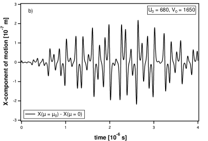
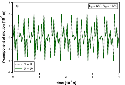
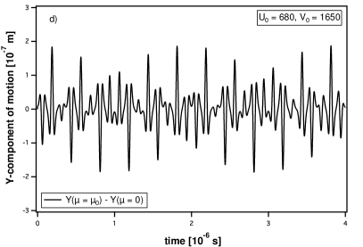
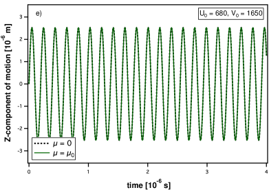
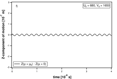
Figure 3: (Color online) Time evolution of the center-of-mass motion of a $\mathrm{MgH^{+}}$ ion inside a linear Paul trap, with classical rotation: (a)–(b) $X$ component of the motion, (c)–(d) $Y$ component of the motion, and (e)–(f) $Z$ component of the motion. In panels (a), (c) and (e), the dotted (black) curves correspond to the trajectories of the ion when $\mu_{0}=0$, while the solid (green) curves show the trajectories when $\mu_{0}\neq 0$. Panels (b), (d), and (f) present the difference between the trajectories, with and without the dipole moment. The magnitudes of the trapping potentials are $U_{0}=$680\text{\,}\mathrm{V}$,V_{0}=$1650\text{\,}\mathrm{V}$$.

As expected from Eqs. (21), one sees that in the presence of a permanent dipole moment, the trajectory of the center of mass does not correspond to the Mathieu equation, which is obtained for $\mu=0$. For such a strength of the trapping field and initial orientation, the deviation is significant enough to be observable in the $x$ direction. However, in the $y$ and $z$ directions the difference between these trajectories is very small compared to the actual amplitudes of the motion. In order to magnify the deviation in the trajectories, especially in the $y$ and $z$ directions, we have plotted the difference between the trajectories with and without the dipole moment in Figs. 3(b), (d), and (f). In the $z$ direction, this difference is small enough to be assumed equal to zero. This arises from the fact that the equation of motion in the $z$ direction, Eq. (21d), lacks the term containing the radio-frequency field, resulting only in a fast-oscillating term (due to the time evolution of $z_{z}^{\prime}$) that averages out to zero. In all cases, the presence of the coupling between the dipole moment and the trapping field does not affect the stability of ion’s trajectory in the trap, which remains bounded and even displays the same oscillation period as when there is no coupling.

Increasing the magnitude of the fields $(U_{0},V_{0})$ increases the magnitude of the interaction energy between the dipole moment and the electric field. Results for the previous field $(U_{0}=$680\text{\,}\mathrm{V}$,V_{0}=$1650\text{\,}\mathrm{V}$)$ are compared to stronger fields in Fig. 4, where we plot the difference in trajectories with and without a dipole moment, only for the $X$ component of motion. To increase visibility, we have only plotted a part of the entire trajectory, in the time interval $[$2.5\text{\,}\mathrm{\SIUnitSymbolMicro s}$,$3.0\text{\,}\mathrm{\SIUnitSymbolMicro s}$]$.

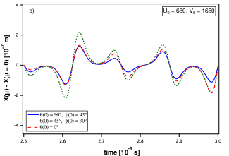
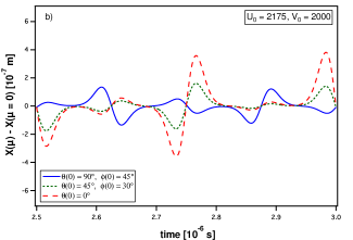
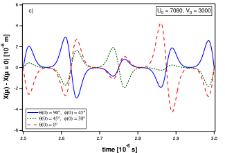
Figure 4: (Color online) Time evolution of the $X$ component of the center-of-mass motion, with classical rotation, for different initial angles and different trap potentials: (a) $U_{0}=$680\text{\,}\mathrm{V}$$, $V_{0}=$1650\text{\,}\mathrm{V}$$; (b) $U_{0}=$2175\text{\,}\mathrm{V}$$, $V_{0}=$2000\text{\,}\mathrm{V}$$; (c) $U_{0}=$7080\text{\,}\mathrm{V}$$, $V_{0}=$3000\text{\,}\mathrm{V}$$. The curves present the difference between the trajectories of motion for the two cases of $\mu=0$ and $\mu=\mu_{0}$.

We see in Fig. 4 that, as expected, the deviation of the trajectories increases with the magnitude of the trapping fields. In the absence of a dipole moment, the trajectories are only moderately affected by the change in the trapping field, while the increased coupling with the dipole moment in the case of the stronger field results in a significant change of trajectory, as evidenced in Fig. 5.

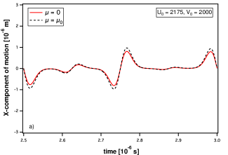
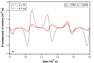
Figure 5: (Color online) Time evolution of the $X$ component of the center-of-mass motion, with classical rotation, for different trap potentials: (a) $U_{0}=$2175\text{\,}\mathrm{V}$$, $V_{0}=$2000\text{\,}\mathrm{V}$$; (b) $U_{0}=$7080\text{\,}\mathrm{V}$$, $V_{0}=$3000\text{\,}\mathrm{V}$$.

We have also investigated the role of the initial orientation of the ion, by changing the initial values of $\theta$ and $\varphi$, as mentioned above. The result is also shown in Fig. 4, where we see a strong dependence of the trajectory on this initial orientation. It is interesting to note that, nevertheless, the deviations in the trajectory show the same periodicity and have the same zero crossings. It appears that the orientation of the dipole significantly changes the trajectory only at the turning points of the latter. As expected, these turning points are also where the rotations are the most hindered by the dipole-field coupling, as evidenced by the rotational energy

$$E_{\mathrm{rot}}=\frac{1}{2}I(\omega_{P{x}^{\prime}}^{2}+\omega_{P{y}^{\prime}}^{2})\,,$$ (34)

see Fig. 6.

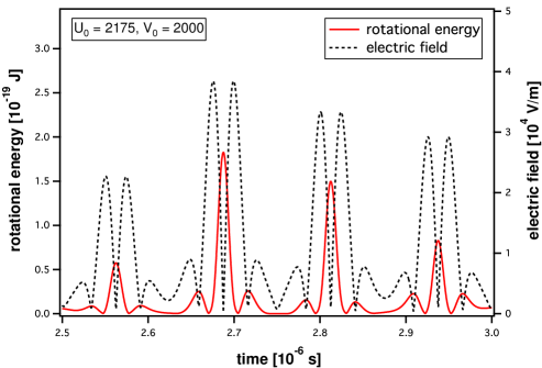
Figure 6: (Color online) Time evolution of the rotational energy of a classical $\mathrm{MgH}^{+}$ molecular ion in a linear Paul trap. The time evolution of the trapping electric field, at the position $\mathbf{R}$ of the ion, is also shown as a dotted (black) curve. The magnitudes of the trapping potentials are $U_{0}=$2175\text{\,}\mathrm{V}$,V_{0}=$2000\text{\,}\mathrm{V}$$.

IV.2 Quantum rotation

In the semi-classical simulations, the initial state of the ion is chosen as for the classical simulations, except for rotations, where we take the initial quantum rotational state to correspond to a specific spherical harmonic $\ket{J,M}$. In other words, all coefficients $D_{J,M}$ in Eq. (25) are equal to zero at $t=0$, except for one which is set to $1$. All the results presented here for the semi-classical model are for the highest magnitude of the trapping field used in the classical simulations, namely $U_{0}=$7080\text{\,}\mathrm{V}$$, $V_{0}=$3000\text{\,}\mathrm{V}$$.

IV.2.1 Effect of the dipole moment on the trajectory

The results for the center-of-mass motion of the ion in the semi-classical model, starting from the initial rotational states $\ket{0,0}$ and $\ket{1,0}$, are shown in Fig. 7. As previously, we also present the difference between the trajectories obtained with and without a dipole moment. Only results along the $X$ and $Y$ axes are presented, as there is no effect on the $Z$ component of the trajectory.

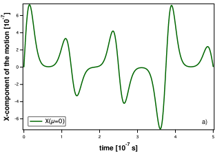
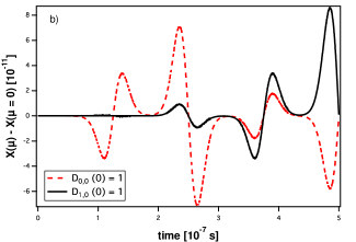
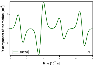
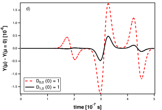
Figure 7: (Color online) Time evolution of the center-of-mass motion of a $\mathrm{MgH^{+}}$ ion inside a linear Paul trap, with quantum rotation, for: (a)–(b) $X$ component of motion, (c)–(d) $Y$ component of motion. Panels (a) and (c) show the trajectories of the motion when $\mu=0$. Panels (b) and (d) present the difference between the trajectories of motion when $\mu=0$ and when $\mu\neq 0$. In the case when $\mu\neq 0$, the ion is initially in a specific rotational state.

Comparing to the result for the classical model, Fig. 4, we see that the effect of the quantum rotation on the center-of-mass motion is smaller. In addition, the deviations in the trajectories are smaller when the ion is initially in an excited state ($J=1$) in comparison to the rotational ground state ($J=0$).

IV.2.2 Effect of the trapping field on the rotation of the ion

We now shift our attention from the center-of-mass motion to the effect of the external trapping electric field on the rotational dynamics of the molecular ion. In Fig. 8, we plot the time evolution of $\left|D_{0,0}(t)\right|^{2}$, the probability of finding the ion in the ground rotational state $\ket{0,0}$.

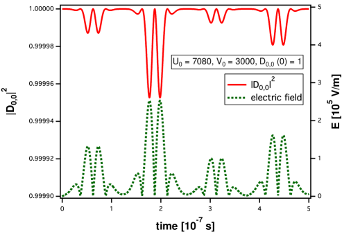
Figure 8: (Color online) Time evolution of the quantum rotational ground state of a $\mathrm{MgH}^{+}$ molecular ion with permanent dipole moment $\mu_{0}$, in a linear Paul trap. The ion is initially in its rotational ground state. The time evolution of the trapping electric field, at the position $\mathbf{R}$ of the ion, is also shown with a dotted (green) curve. The magnitudes of the trapping potentials are $U_{0}=$7080\text{\,}\mathrm{V}$,V_{0}=$3000\text{\,}\mathrm{V}$$.

We see that the trapping field causes a small perturbation in the quantum rotation of the diatomic ion, as is clearly evidenced by the local value of the field felt by the ion, which is also plotted in Fig. 8. The trapping field is thus coupling the ground rotational state to excited states, but the ion appears to return adiabatically to the ground state as it revisits a low-field region.

Comparable results are obtained when starting from the excited states $\ket{1,0}$ or $\ket{1,1}$, as shown in Fig. 9.

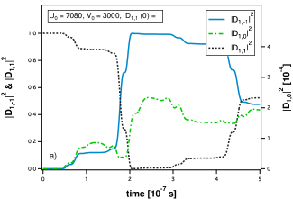
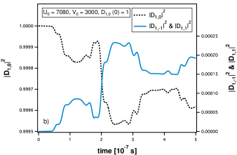
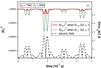
Figure 9: (Color online) Time evolution of the first excited quantum rotational state of a $\mathrm{MgH}^{+}$ molecular ion with permanent dipole moment $\mu_{0}$, in a linear Paul trap. Panels (a)–(b) show the time evolution of sub-levels $M=0,\pm 1$ when the ion is initially in either rotational states corresponding to $J=1$, $M=1$ [panel (a)] and $J=1$, $M=0$ [panel(b)]. Panel (c) compares the time evolution of state with $J=1$, for the two initial conditions mentioned, along with the time evolution of the trapping electric field at the position $\mathbf{R}$ of the ion. The magnitudes of the trapping potentials are $U_{0}=$7080\text{\,}\mathrm{V}$,V_{0}=$3000\text{\,}\mathrm{V}$$.

Starting from the state $\ket{1,1}$, one sees, Fig. 9(a), a strong exchange with the corresponding sub-level with opposite $M=-1$, $\ket{1,-1}$, with limited transfer to the state $\ket{1,0}$ [note the difference in scale in Fig. 9(a) for the latter state]. Similarly, starting from $\ket{1,0}$, the ion basically stays in that state, as shown in Fig. 9(b).

By summing over the probabilities of finding the ion to be in one of the sub-levels above, i.e.,

$$\left|D_{J}(t)\right|^{2}\equiv\sum_{M=-J}^{J}\left|D_{J,M}(t)\right|^{2}$$ (35)

for $J=1$, we see in Fig. 9(c) that the excited states are less perturbed by the external field than the ground state, especially when starting from $\ket{1,0}$. Nevertheless, the states corresponding to $J=1$ follow the same temporal changes as the local electric field, as was the case for the ground state.

Finally, we have also compared the time evolution of the first three rotational states of the ion corresponding to quantum numbers $J=0$, $J=1$ and $J=2$, by studying their populations $\left|D_{J}(t)\right|^{2}$, Eq. (35), in Fig. 10.

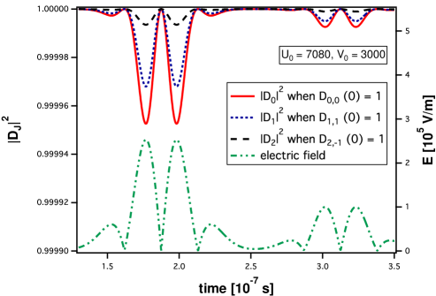
Figure 10: (Color online) Comparison of the time evolution of the quantum rotational ground state $J=0$ (when the ion is initially in this state), first rotational excited state $J=1$ (when the ion is initially in this state), and second rotational excited state $J=2$ (when the ion is initially in this state) with each other and with the time evolution of the trapping electric field, at the position $\mathbf{R}$ of the ion. The magnitudes of the trapping potentials are $U_{0}=$7080\text{\,}\mathrm{V}$,V_{0}=$3000\text{\,}\mathrm{V}$$.

As we see, the rotational ground state is the most affected state by the interaction of the electric field with the dipole, while on the other hand, the states corresponding to $J=2$ are hardly affected by the trapping field. This confirms the tendency that was seen in Figs. 8 and 9, that the higher the energy of the rotational state, the less it is affected by the interaction between the trapping electric field and the dipole moment. It can be understood by considering that the lower the value of $J$, the more the presence of the dipole-field interaction $\bm{\mu}\cdot\mathbf{E}$ affects the rotational eigenstates, see Refs. von Meyenn, 1970; Friedrich and Herschbach, 1991.

V Conclusion

We have studied the dynamics of a rigid heteronuclear diatomic molecular ion trapped in a linear Paul trap by carrying out both classical and semi-classical numerical simulations. We have investigated the effect of the interaction between the permanent dipole moment of the ion and the time-varying trapping electric field on the motion of the center of mass of the ion, along with the effect of the field on the rotation of the ion.

Classically, we showed that the trajectories of the center of mass differ from those of an equivalent ion without a permanent dipole moment. The trajectories obtained therefore do not follow the Mathieu equation, as atomic ions do, but present nevertheless the same periodic oscillations. We observed that the deviation of the trajectories of the motion of the molecular ion is strongly dependent on its initial orientation (orientation of the dipole) inside the trap, for the same magnitude of the electric field. Similarly, a stronger trapping field lead to a greater divergence between the trajectories with and without a coupling between the field and the dipole moment of the ion.

Considering quantum rotation in a semi-classical model, we found that the time evolution of the rotational states of the ion follows closely the time evolution of the trapping electric field. Therefore, when the electric field is zero, the initial rotational state of the ion is fully populated and as soon as the electric field increases from zero, the probability of finding the ion in other rotational states becomes non-zero. We showed that higher rotational states of the ion are less affected by the interaction of the dipole moment with the trapping electric field. We also found that the trajectory of the ion is less affected by the coupling between the trapping field and the dipole moment when quantum rotation is considered, compared to classical rotation.

In all cases, we found that the deviations of the trajectories from the Mathieu equation did not lead to unbounded trajectories. In other words, the stability of the trap was not affected by the presence of the coupling between the dipole moment and the trapping field for the potential values $U_{0}$ and $V_{0}$ used in this study. Future work should explore whether there exists instances where this is not the case, maybe very close to the border between stable and unstable trajectories.

Appendix A Classical model for a dipolar rigid rotor in an external electric field

A.1 Definition of the model

We represent a dipolar diatomic molecular ion as a classical rigid rotor, with two partial charges $\delta_{+}$ and $\delta_{-}$ located at $\mathbf{r}_{+}$ and $\mathbf{r}_{-}$, see Fig. 11.

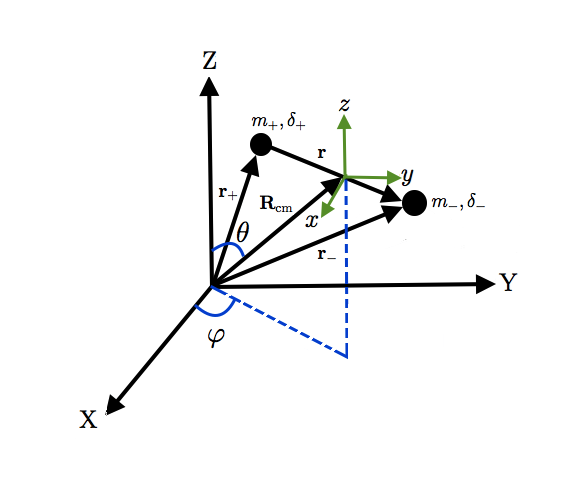
Figure 11: (Color online) Representation of a dipolar, diatomic molecular ion as a system of two masses $m_{+}$ and $m_{-}$ possessing charges $\delta_{+}$ and $\delta_{-}$, respectively.

In order to reproduce the characteristics of the molecular ion, $r\equiv\left|\mathbf{r}\right|$ is fixed to the internuclear distance, with $\mathbf{r}\equiv\mathbf{r}_{+}-\mathbf{r}_{-}$, and the two charges are assigned the masses $m_{+}$ and $m_{-}$ of the corresponding atoms. The position of the center of mass is given by

$$\mathbf{R}=\frac{m_{+}\mathbf{r}_{+}+m_{-}\mathbf{r}_{-}}{m_{+}+m_{-}}=\frac{m_{+}\mathbf{r}_{+}+m_{-}\mathbf{r}_{-}}{M},$$ (36)

where $M\equiv m_{+}+m_{-}$ is the total mass of the molecular ion. The position of the partial charges relative to the center of mass, $\mathbf{r}^{\prime}_{\pm}$, are obtained from

$$\mathbf{r}_{\pm}=\mathbf{R}+\mathbf{r}^{\prime}_{\pm},$$ (37)

from which we get

$$m_{+}\mathbf{r}_{+}+m_{-}\mathbf{r}_{-}=M\mathbf{R}+m_{+}\mathbf{r}_{+}^{\prime}+m_{-}\mathbf{r}_{-}^{\prime},$$ (38)

so by definition of the center of mass, we have that

$$m_{+}\mathbf{r}_{+}^{\prime}+m_{-}\mathbf{r}_{-}^{\prime}=0.$$ (39)

Similarly, starting from the momentum

$$m_{+}\dot{\mathbf{r}}_{+}+m_{-}\dot{\mathbf{r}}_{-}=M\dot{\mathbf{R}},$$ (40)

we deduce that

$$m_{+}\dot{\mathbf{r}}_{+}^{\prime}+m_{-}\dot{\mathbf{r}}_{-}^{\prime}=0$$ (41)

Using the above definitions, we can find the partial charges by imposing that

$$\delta_{+}+\delta_{-}=Ze,$$ (42)

with $Ze$ the total charge of the ion and $e$ the elementary charge, along with

$$\delta_{+}\mathbf{r}_{+}^{\prime}+\delta_{-}\mathbf{r}_{-}^{\prime}=\bm{\mu},$$ (43)

with $\bm{\mu}$ the dipole moment of the molecular ion.

A.1.1 Center-of-mass frame

We define an additional reference frame $(x,y,z)$ centered on the center of mass of the molecular ion, that remains aligned with the lab reference frame $(X,Y,Z)$, i.e., $\mathbf{\hat{x}}$ is always parallel to $\mathbf{\hat{X}}$, etc., where the $\mathbf{\hat{\mbox{ }}}$ denotes unit vectors. In the center-of-mass frame, the vector $\mathbf{r}_{+}$ can be expressed in spherical coordinates as

$$\mathbf{r}_{+}=\mathbf{\hat{x}}r_{+}^{\prime}\sin\theta\cos\varphi+\mathbf{\hat{y}}r_{+}^{\prime}\sin\theta\sin\varphi+\mathbf{\hat{z}}r_{+}^{\prime}\cos\theta,$$ (44)

with its time derivative

$$\dot{\mathbf{r}}_{+} =\mathbf{\hat{x}}r_{+}^{\prime}\left(\dot{\theta}\cos\theta\cos\varphi-\dot{\varphi}\sin\theta\sin\varphi\right)$$

$$\quad+\mathbf{\hat{y}}r_{+}^{\prime}\left(\dot{\theta}\cos\theta\sin\varphi+\dot{\varphi}\sin\theta\cos\varphi\right)$$

$$\quad+\mathbf{\hat{z}}r_{+}^{\prime}\left(-\dot{\theta}\sin\theta\right),$$ (45)

where we have made use of the rigid rotor approximation, $\dot{r}_{+}^{\prime}=0$. From this, we get

$$\dot{\mathbf{r}}_{+}\cdot\dot{\mathbf{r}}_{+} =\left(r_{+}^{\prime}\right)^{2}\left[\left(\dot{\theta}\cos\theta\cos\varphi-\dot{\varphi}\sin\theta\sin\varphi\right)^{2}\right.$$

$$\quad\quad\quad+\left(\dot{\theta}\cos\theta\sin\varphi+\dot{\varphi}\sin\theta\cos\varphi\right)^{2}$$

$$\quad\quad\quad\left.+\left(-\dot{\theta}\sin\theta\right)^{2}\right],$$

which, after some simple algebra, results in

$$=\left(r_{+}^{\prime}\right)^{2}\left[\dot{\theta}^{2}+\dot{\varphi}^{2}\sin^{2}\theta\right].$$ (46)

For $\mathbf{r}_{-}$, we have to make the substitutions $\theta\rightarrow\pi-\theta$ and $\varphi\rightarrow\varphi+\pi$, hence

$$\mathbf{r}_{-}=-\mathbf{\hat{x}}r_{-}^{\prime}\sin\theta\cos\varphi-\mathbf{\hat{y}}r_{-}^{\prime}\sin\theta\sin\varphi-\mathbf{\hat{z}}r_{-}^{\prime}\cos\theta,$$ (47)

from which we recover

$$\dot{\mathbf{r}}_{-}\cdot\dot{\mathbf{r}}_{-}=\left(r_{-}^{\prime}\right)^{2}\left[\dot{\theta}^{2}+\dot{\varphi}^{2}\sin^{2}\theta\right].$$ (48)

A.2 Kinetic energy

Using the notation $\mathbf{v}\equiv\dot{\mathbf{r}}$, the kinetic energy is given by

$$K =\frac{1}{2}\left(m_{+}v_{+}^{2}+m_{-}v_{-}^{2}\right)$$

$$=\frac{1}{2}\left(m_{+}\mathbf{v}_{+}\cdot\mathbf{v}_{+}+m_{-}\mathbf{v}_{-}\cdot\mathbf{v}_{-}\right)$$

$$=\frac{1}{2}\left[m_{+}\left(\dot{\mathbf{R}}\cdot\dot{\mathbf{R}}+2\dot{\mathbf{R}}\cdot\dot{\mathbf{r}}_{+}^{\prime}+\dot{\mathbf{r}}_{+}^{\prime}\cdot\dot{\mathbf{r}}_{+}^{\prime}\right)+m_{-}\left(\dot{\mathbf{R}}\cdot\dot{\mathbf{R}}+2\dot{\mathbf{R}}\cdot\dot{\mathbf{r}}_{-}^{\prime}+\dot{\mathbf{r}}_{-}^{\prime}\cdot\dot{\mathbf{r}}_{-}^{\prime}\right)\right]$$

$$=\frac{1}{2}\left[MV^{2}+2\dot{\mathbf{R}}\cdot\left(m_{+}\dot{\mathbf{r}}_{+}^{\prime}+m_{-}\dot{\mathbf{r}}_{-}^{\prime}\right)+m_{+}v_{+}^{\prime 2}+m_{-}v_{-}^{\prime 2}\right]$$

$$=\frac{1}{2}\left(MV^{2}+m_{+}v_{+}^{\prime 2}+m_{-}v_{-}^{\prime 2}\right),$$ (49)

where we have used Eq. (41). Using Eqs. (46) and (48), we can express the kinetic energy in spherical coordinates as

$$K =\frac{1}{2}\left(M\dot{\mathbf{R}}^{2}+m_{+}\dot{\mathbf{r}}_{+}^{\prime 2}+m_{-}\dot{\mathbf{r}}_{-}^{\prime 2}\right)$$

$$=\frac{1}{2}M\dot{\mathbf{R}}^{2}+\frac{1}{2}\left(m_{+}r_{+}^{\prime 2}+m_{-}r_{-}^{\prime 2}\right)\left(\dot{\theta}^{2}+\dot{\varphi}^{2}\sin^{2}\theta\right).$$ (50)

From the definition of the center of mass, we have

$$m_{+}r_{+}^{\prime 2}+m_{-}r_{-}^{\prime 2} =m_{+}\left(\frac{m_{-}}{M}r\right)^{2}+m_{-}\left(\frac{m_{+}}{M}r\right)^{2}$$

$$=\frac{m_{+}m_{-}^{2}}{M^{2}}r^{2}+\frac{m_{-}m_{+}^{2}}{M^{2}}r^{2}$$

$$=\frac{m_{+}m_{-}}{M}\left(\frac{m_{+}+m_{-}}{M}\right)r^{2}$$

$$=m_{\mathrm{red}}r^{2}$$ (51)

where the reduced mass $m_{\mathrm{red}}\equiv m_{+}m_{-}/M$. We thus get

$$K =\frac{1}{2}M\dot{\mathbf{R}}^{2}+\frac{1}{2}m_{\mathrm{red}}r^{2}\left(\dot{\theta}^{2}+\dot{\varphi}^{2}\sin^{2}\theta\right)$$

$$=\frac{1}{2}M\dot{\mathbf{R}}^{2}+\frac{1}{2}I\dot{\bm{\omega}}^{2},$$ (52)

where $I\equiv m_{\mathrm{red}}r^{2}$ is the moment of inertia and $\dot{\bm{\omega}}$ the angular velocity.

A.3 Potential energy

We consider only the interaction of the partial charges $\delta_{\pm}$ with an external electric field $\Phi$,

$$V=\delta_{+}\Phi(\mathbf{r}_{+})+\delta_{-}\Phi(\mathbf{r}_{-}).$$ (53)

Considering the form of the electric potential inside a Paul trap [see Eqs. (1) and (2)], we can separate it into Cartesian components

$$\Phi(X,Y,Z)=\Phi_{X}X^{2}+\Phi_{Y}Y^{2}+\Phi_{Z}Z^{2},$$ (54)

such that the Taylor expansion of $\Phi(\mathbf{r}_{\pm})=\Phi(\mathbf{R}+\mathbf{r}_{\pm}^{\prime})$ around the center of mass is given by

$$\Phi(\mathbf{R}+\mathbf{r}_{\pm}^{\prime}) =\Phi(\mathbf{R})+(\mathbf{r}_{\pm}^{\prime})_{x}\left.\frac{\partial}{\partial x}\Phi\right|_{\mathbf{R}}+(\mathbf{r}_{\pm}^{\prime})_{y}\left.\frac{\partial}{\partial y}\Phi\right|_{\mathbf{R}}+(\mathbf{r}_{\pm}^{\prime})_{z}\left.\frac{\partial}{\partial z}\Phi\right|_{\mathbf{R}}$$

$$\quad+(\mathbf{r}_{\pm}^{\prime})_{x}^{2}\left.\frac{\partial^{2}}{\partial x^{2}}\Phi\right|_{\mathbf{R}}+(\mathbf{r}_{\pm}^{\prime})_{y}^{2}\left.\frac{\partial^{2}}{\partial y^{2}}\Phi\right|_{\mathbf{R}}+(\mathbf{r}_{\pm}^{\prime})_{z}^{2}\left.\frac{\partial^{2}}{\partial z^{2}}\Phi\right|_{\mathbf{R}}$$ (55)

with higher-order terms all zero. In deriving the previous equation, we have made use of the fact that the coordinate systems $(X,Y,Z)$ and $(x,y,z)$ are parallel, such that the operators $\partial/\partial X$ and $\partial/\partial x$ are equivalent, etc. We finally get

$$V =(\delta_{+}+\delta_{-})\Phi(\mathbf{R})+\sum_{\xi=x,y,z}\left[\delta_{+}(\mathbf{r}_{+}^{\prime})_{\xi}+\delta_{-}(\mathbf{r}_{-}^{\prime})_{\xi}\right]\left.\frac{\partial}{\partial\xi}\Phi\right|_{\mathbf{R}}$$

$$\quad+\sum_{\xi=x,y,z}\left[\delta_{+}(\mathbf{r}_{+}^{\prime})_{\xi}^{2}+\delta_{-}(\mathbf{r}_{-}^{\prime})_{\xi}^{2}\right]\left.\frac{\partial^{2}}{\partial\xi^{2}}\Phi\right|_{\mathbf{R}}$$

$$=Ze\Phi(\mathbf{R})+\bm{\mu}\cdot\left.\bm{\nabla}\Phi\right|_{\mathbf{R}}+\ldots$$

$$\approx Ze\Phi(\mathbf{R})-\bm{\mu}\cdot\mathbf{E}(\mathbf{R}),$$ (56)

where we have made use of Eqs. (42) and (43), along with the relation for the electric field $\mathbf{E}=-\nabla\Phi$. Neglecting term including the second derivative of the potential with respect to the coordinates, which is the gradient of the field, corresponds to approximating the system as a point dipole.

References

- Mølhave and Drewsen (2000) K. Mølhave and M. Drewsen, “Formation of translationally cold MgH+ and MgD+ molecules in an ion trap,” Phys. Rev. A 62, 011401 (2000).
- Blythe et al. (2005) P. Blythe, B. Roth, U. Fröhlich, H. Wenz, and S. Schiller, “Production of ultracold trapped molecular hydrogen ions,” Phys. Rev. Lett. 95, 183002 (2005).
- Baba and Waki (2002) T. Baba and I. Waki, “Chemical reaction of sympathetically laser-cooled molecular ions,” J. Chem. Phys. 116, 1858–1861 (2002).
- Tong et al. (2012) X. Tong, T. Nagy, J. Y. Reyes, M. Germann, M. Meuwly, and S. Willitsch, “State-selected ion-molecule reactions with Coulomb-crystallized molecular ions in traps,” Chem. Phys. Lett. 547, 1–8 (2012).
- Chang et al. (2013) Y.-P. Chang, K. Długołȩcki, J. Küpper, D. Rösch, D. Wild, and S. Willitsch, “Specific chemical reactivities of spatially separated 3-aminophenol conformers with cold Ca+ ions,” Scienc 342, 98–101 (2013).
- Rösch et al. (2014) D. Rösch, S. Willitsch, Y.-P. Chang, and J. Küpper, “Chemical reactions of conformationally selected 3-aminophenol molecules in a beam with Coulomb-crystallized Ca+ ions,” J. Chem. Phys. 140, 124202 (2014).
- Douglas, Frank, and Mao (2005) D. J. Douglas, A. J. Frank, and D. Mao, “Linear ion traps in mass spectrometry,” Mass Spectro. Rev. 24, 1–29 (2005).
- Leanhardt et al. (2011) A. E. Leanhardt, J. L. Bohn, H. Loh, P. Maletinsky, E. R. Meyer, L. C. Sinclair, R. P. Stutz, and E. A. Cornell, “High-resolution spectroscopy on trapped molecular ions in rotating electric fields: A new approach for measuring the electron electric dipole moment,” J. Mol. Spectrosc. 270, 1–25 (2011).
- Loh et al. (2013) H. Loh, K. C. Cossel, M. C. Grau, K.-K. Ni, E. R. Meyer, J. L. Bohn, J. Ye, and E. A. Cornell, “Precision spectroscopy of polarized molecules in an ion trap,” Science 342, 1220–1222 (2013).
- Weidinger and Gruebele (2008) D. Weidinger and M. Gruebele, “Simulations of quantum computation with a molecular ion,” Chem. Phys. 350, 139–144 (2008).
- Buluta et al. (2008) I. M. Buluta, M. Kitaoka, S. Georgescu, and S. Hasegawa, “Investigation of planar Coulomb crystals for quantum simulation and computation,” Phys. Rev. A 77, 062320 (2008).
- Alonso et al. (2013) J. Alonso, F. M. Leupold, B. C. Keitch, and J. P. Home, “Quantum control of the motional states of trapped ions through fast switching of trapping potentials,” New J. Phys. 15, 023001 (2013).
- Amniat-Talab, Saadati-Niari, and Guérin (2012) M. Amniat-Talab, M. Saadati-Niari, and S. Guérin, “Quantum state engineering in ion-traps via adiabatic passage,” Eur. Phys. J. D 66, 1–9 (2012).
- Leibfried (2012) D. Leibfried, “Quantum state preparation and control of single molecular ions,” New J. Phys. 14, 023029 (2012).
- Shi et al. (2013) M. Shi, P. F. Herskind, M. Drewsen, and I. L. Chuang, “Microwave quantum logic spectroscopy and control of molecular ions,” New J. Phys. 15, 113019 (2013).
- Paul (1990) W. Paul, “Electromagnetic traps for charged and neutral particles,” Rev. Mod. Phys. 62, 531–540 (1990).
- Prestage, Dick, and Maleki (1989) J. D. Prestage, G. J. Dick, and L. Maleki, “New ion trap for frequency standard applications,” J. Appl. Phys. 66, 1013–1017 (1989).
- Raizen et al. (1992a) M. G. Raizen, J. M. Gilligan, J. C. Bergquist, W. M. Itano, and D. J. Wineland, “Ionic crystals in a linear Paul trap,” Phys. Rev. A 45, 6493–6501 (1992a).
- Raizen et al. (1992b) M. G. Raizen, J. M. Gilligan, J. C. Bergquist, W. M. Itano, and D. J. Wineland, “Linear trap for high-accuracy spectroscopy of stored ions,” J. Mod. Opt. 39, 233–242 (1992b).
- Brkić et al. (2006) B. Brkić, S. Taylor, J. F. Ralph, and N. France, “High-fidelity simulations of ion trajectories in miniature ion traps using the boundary-element method,” Phys. Rev. A 73, 012326 (2006).
- Drewsen et al. (2003) M. Drewsen, I. Jensen, J. Lindballe, N. Nissen, R. Martinussen, A. Mortensen, P. Staanum, and D. Voigt, “Ion Coulomb crystals: a tool for studying ion processes,” Int. J. Mass Spectrom. 229, 83–91 (2003).
- Porras and Cirac (2006) D. Porras and J. I. Cirac, “Quantum manipulation of trapped ions in two dimensional Coulomb crystals,” Phys. Rev. Lett. 96, 250501 (2006).
- Willitsch (2012) S. Willitsch, “Coulomb-crystallised molecular ions in traps: methods, applications, prospects,” Int. Rev. Phys. Chem. 31, 175–199 (2012).
- Vogelius, Madsen, and Drewsen (2006) I. S. Vogelius, L. B. Madsen, and M. Drewsen, “Rotational cooling of molecular ions through laser-induced coupling to the collective modes of a two-ion Coulomb crystal,” J. Phys. B 39, S1267–S1280 (2006).
- Lazarou, Keller, and Garraway (2010) C. Lazarou, M. Keller, and B. M. Garraway, “Molecular heat pump for rotational states,” Phys. Rev. A 81, 013418 (2010).
- Berglund, Drewsen, and Koch (2015) J. M. Berglund, M. Drewsen, and C. P. Koch, “Femtosecond wavepacket interferometry using the rotational dynamics of a trapped cold molecular ion,” New J. Phys. 17, 025007 (2015).
- Evans (1977) D. J. Evans, “On the representation of orientation space,” Mol. Phys. 34, 317–325 (1977).
- Major, Gheorghe, and Werth (2005) F. G. Major, V. N. Gheorghe, and G. Werth, Charged Particle Traps: Physics and Techniques of Charged Particle Field Confinement (Springer, Berlin, 2005).
- Ghosh (1995) P. K. Ghosh, Ion Traps (Oxford University Press, Oxford, 1995).
- Hashemloo, Dion, and Rahali (2016) A. Hashemloo, C. M. Dion, and G. Rahali, “Wave-packet dynamics of an atomic ion in a Paul trap: Approximations and stability,” Int. J. Mod. Phys. C 27, 1650014 (2016).
- Wolf (2010) G. Wolf, “Mathieu functions and Hill’s equation,” in NIST Handbook of Mathematical Functions, edited by F. W. J. Oliver, D. W. Lozier, R. F. Boisvert, and C. W. Clark (Cambridge University Press, Cambridge, 2010) Chap. 28, pp. 651–681.
- Cheung and Powles (1975) P. S. Y. Cheung and J. G. Powles, “The properties of liquid nitrogen,” Mol. Phys. 30, 921–949 (1975).
- Cheung (1976) P. S. Y. Cheung, “On the efficient evaluation of torques and forces for anisotropic potentials in computer simulation of liquids composed of linear molecules,” Chem. Phys. Lett. 40, 19 – 22 (1976).
- Evans and Murad (1977) D. J. Evans and S. Murad, “Singularity free algorithm for molecular dynamics simulation of rigid polyatomics,” Mol. Phys. 34, 327–331 (1977).
- Goldstein, Poole, and Safko (2002) H. Goldstein, C. P. Poole, and J. L. Safko, Classical Mechanics, 3rd ed. (Addison Wesley, San Francisco, 2002).
- Combescure (1986) M. Combescure, “A quantum particle in a quadrupole radio-frequency trap,” Ann. Inst. Henri Poincaré, A 44, 293–314 (1986).
- Brown (1991) L. S. Brown, “Quantum motion in a Paul trap,” Phys. Rev. Lett. 66, 527–529 (1991).
- Glauber (1992) R. J. Glauber, “The quantum mechanics of trapped wave packets,” in Laser Manipulation of Atoms and Ions, edited by E. Arimondo, W. D. Phillips, and F. Strumia (North-Holland, Amsterdam, 1992) pp. 643–660.
- Varshalovich, Moskalev, and Khersonskiĭ (1988) D. A. Varshalovich, A. N. Moskalev, and V. K. Khersonskiĭ, Quantum Theory of Angular Momentum (World Scientific, Singapore, 1988).
- Press et al. (1992) W. H. Press, S. A. Teukolsky, W. T. Vetterling, and B. P. Flannery, Numerical Recipes in C, 2nd ed. (Cambridge University Press, Cambridge, 1992).
- Galassi et al. (2009) M. Galassi et al., GNU Scientific Library Reference Manual, 3rd ed. (Network Theory, Bristol, 2009).
- Bertelsen, Jørgensen, and Drewsen (2006) A. Bertelsen, S. Jørgensen, and M. Drewsen, “The rotational temperature of polar molecular ions in Coulomb crystals,” J. Phys. B 39, L83 (2006).
- Abe et al. (2010) M. Abe, M. Kajita, M. Hada, and Y. Moriwaki, “Ab initio study on vibrational dipole moments of XH+ molecular ions: X = 24Mg, 40Ca, 64Zn, 88Sr, 114Cd, 138Ba, 174Yb and 202Hg,” J. Phys. B 43, 245102 (2010).
- Højbjerre et al. (2009) K. Højbjerre, A. K. Hansen, P. S. Skyt, P. F. Staanum, and M. Drewsen, “Rotational state resolved photodissociation spectroscopy of translationally and vibrationally cold MgH+ ions: toward rotational cooling of molecular ions,” New J. Phys. 11, 055026 (2009).
- von Meyenn (1970) K. von Meyenn, “Rotation von zweiatomigen Dipolmolekülen in starken elektrischen Feldern,” Z. Phys. 231, 154–160 (1970).
- Friedrich and Herschbach (1991) B. Friedrich and D. R. Herschbach, “On the possibility of orienting rotationally cooled polar molecules in an electric field,” Z. Phys. D 18, 153–161 (1991).