Inverted initial conditions: exploring the growth of cosmic structure and voids

Abstract

We introduce and explore “paired” cosmological simulations. A pair consists of an A and B simulation with initial conditions related by the inversion $\delta_{A}(\bm{\mathbf{x}},t_{\mathrm{initial}})=-\delta_{B}(\bm{\mathbf{x}},t_{\mathrm{initial}})$ (underdensities substituted for overdensities and vice versa). We argue that the technique is valuable for improving our understanding of cosmic structure formation. The A and B fields are by definition equally likely draws from $\Lambda$CDM initial conditions, and in the linear regime evolve identically up to the overall sign. As non-linear evolution takes hold, a region that collapses to form a halo in simulation A will tend to expand to create a void in simulation B. Applications include (i) contrasting the growth of A-halos and B-voids to test excursion-set theories of structure formation; (ii) cross-correlating the density field of the A and B universes as a novel test for perturbation theory; and (iii) canceling error terms by averaging power spectra between the two boxes. Generalizations of the method to more elaborate field transformations are suggested.

I Introduction

The interpretation of cosmological observations increasingly requires a precise understanding of non-linear structure formation. In addition to the power spectrum of the matter distribution, the properties and abundances of non-linear structures such as clusters Planck Collaboration et al. (2015a) or voids Lavaux and Wandelt (2012) also have the potential to constrain cosmological parameters.

Excursion-set theories Press and Schechter (1974); Bond et al. (1991); Zentner (2007) suggest that the formation of voids from initial underdensities is nearly but not precisely analogous to the formation of halos from overdensities Sheth and van de Weygaert (2004); Furlanetto and Piran (2006); Paranjape et al. (2012); Jennings et al. (2013). The imperfect symmetry suggests that directly contrasting void and halo formation could be informative. In this work we take a first step in this direction by comparing results from two simulations with precisely opposite initial conditions (underdensities substituted for overdensities and vice versa). We refer to these simulations as being “paired”.

The paired simulations can also be used to improve both practical estimation and theoretical understanding of the matter power spectrum (and higher order correlations). There are presently two approaches to calculating the non-linear power spectrum: analytic perturbation theory, or computational N-body simulations. The former comes in a wide variety of flavours, because the simplest perturbative treatment of gravitational instability (standard perturbation theory, SPT Bernardeau et al. (2002)) suffers from divergences at increasing comoving wavenumber $k$. These can be brought under control by partially resumming some of the SPT series Crocce and Scoccimarro (2006a) or writing down an effective theory Carrasco et al. (2012). The resulting theories can be tested or calibrated on simulations Nishimichi et al. (2009); Carlson et al. (2009); Roth and Porciani (2011); Gil-Marín et al. (2012); Vlah et al. (2015); Foreman et al. (2015).

The most familiar example of a non-standard perturbation theory is the Zel’dovich approximation, a linear expansion in Lagrangian space which leads to a regrouping of terms. While the raw Zel’dovich predictions for the auto-power spectrum are inaccurate, in many respects it behaves better than Eulerian perturbation theory Buchert (1992); Crocce and Scoccimarro (2006a); Matsubara (2008). In particular, it correctly predicts the decay of the cross-correlation between initial conditions and the final non-linear field Crocce and Scoccimarro (2006a); Bernardeau et al. (2008); Matsubara (2008); Carlson et al. (2009); White (2014). In the present work we cross-correlate the non-linear density fields of the paired simulations, providing an alternative performance comparison of different perturbative schemes from a physical perspective. We find that the Zel’dovich approximation continues to offer insight in this new regime.

From a purely practical perspective the science case for forthcoming large scale structure surveys requires percent-level accuracy on computations even on strongly non-linear, megaparsec scales Schneider et al. (2015). Our third application for paired simulations shows how they can be used to cancel a large class of finite-volume errors that can compromise this requirement. The same cancellation can be approximately achieved by averaging over a large ensemble of uncorrelated simulations, but the paired approach is more computationally efficient.

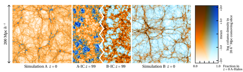
Figure 1: An illustration of the paired simulation technique. A standard $\Lambda$CDM simulation is performed as described in the text. The left panel shows the present day ($z=0$) projected density field in a $20\,h^{-1}\ \mathrm{Mpc}$ slice through the simulation. Collapsed dark matter halos have been identified using a friends-of-friends algorithm; the fraction of the column density contributed by particles in such structures is color-coded from orange (no contribution) to blue (100% contribution). The center-left panel shows the initial conditions, color-coded according to the same scheme. The initial conditions for the B simulation are obtained by reversing the sign of the overdensity field (center-right panel). While the statistical properties of the linear field are unchanged by this transformation, the blue “A-halo” particles are now associated with underdensities. Evolving the B-simulation to $z=0$ gives rise to the right panel. The B-voids are seen to be associated with the same particles (i.e., the same Lagrangian regions) as the A-halos.

After describing the simulation setup (Section II) we discuss the asymmetry in the evolution of halos and voids (Section II.1) and then show how the technique generates new insights into perturbation theory (Section II.2) and improves the accuracy of power spectrum estimates (Section II.3). Possible extensions to the technique are discussed in Section III. We conclude in Section IV.

II Results

In this paper we present results from paired cosmological simulations drawn from an ensemble described by the WMAP 7-year recommended cosmological parameters Komatsu et al. (2011) (“WMAP+BAO+$H_{0}$ ML”). While these are no longer the most precise parameters available Planck Collaboration et al. (2015b), they are sufficiently close for our present purposes where we do not compare to observational data; adopting WMAP7 parameters allowed us to make use of an existing simulation which we refer to as “A”. We perform dark-matter-only simulations, adding the baryon density to that of the dark matter.

We used CAMB (Lewis et al., 2000) to generate the initial power spectrum of fluctuations from which we drew a random realization $\bm{\mathbf{\delta}}_{S}(x,t_{\mathrm{initial}})$ on a uniform $512^{3}$ grid in a $(200\,h^{-1}\,\mathrm{Mpc})^{3}$ volume, so probing wavenumbers $0.031<k/(h\ \mathrm{Mpc}^{-1})<16$. The initial particle displacements and velocities were generated using the Zel’dovich approximation at redshift $z=99$, deep in the linear regime for the relevant scales. All simulations were run to $z=0$ using the P-Gadget-3 code (Springel, 2005; Springel et al., 2008). The particle softening was set to $\epsilon=5\,h^{-1}\,\mathrm{kpc}$. Halos were identified with the subfind algorithm Springel et al. (2001).

We generated the initial conditions for the first simulation (denoted “A”) using the same code as Ref. Roth et al. (2015) and flipped the sign of the overdensity to generate the “B” initial conditions, $\bm{\mathbf{\delta}}_{B}(x,t_{\mathrm{initial}})=-\bm{\mathbf{\delta}}_{A}(x,t_{\mathrm{initial}})$. Both simulations are on an equal footing in the sense that they are equally probable draws from the underlying statistical description of the initial conditions. However, their relationship with each other allows for systematic investigations into various aspects of structure formation as we describe in the following sections.

II.1 Evolution of anti-halos

To begin our study of the relationship between the A and B simulations, we show that halos map reliably onto voids (and vice versa). This situation is illustrated in Fig. 1 which shows, from left to right, a $20\,h^{-1}\,\mathrm{Mpc}$ slice through the matter density field of the $z=0$ A-simulation, the $z=99$ A-simulation, the $z=99$ B-simulation and the $z=0$ B-simulation. The brightness represents projected mass density while colors track the fraction of particles identified as halos in the A-simulation. The voids in the B simulation are identified as A-halo-dominated regions (colored blue) interspersed by filaments, which are A-halo-free regions (colored orange). This relationship is symmetric: a similar figure can be made starting from the halos in the B simulation.

Figure 1 suggests that voids in the B simulation can be identified with “anti-halos”, i.e., the Lagrangian region defined by the particles making up A-halos. However, theories of structure formation using the excursion set formalism emphasise that there is an asymmetry between the evolution of halos and voids Sheth and van de Weygaert (2004); Furlanetto and Piran (2006); Paranjape et al. (2012): voids can be crushed by a large-scale overdensity that collapses at late times, whereas halos are not erased by living in a large-scale void.

The A/B comparison allows us to search for direct evidence of this asymmetry. We take the $z=0$ A-halos in three mass bins: $10^{14}<M/M_{\odot}<10^{15}$, $10^{13}<M/M_{\odot}<10^{14}$ and $10^{12}<M/M_{\odot}<10^{13}$; there are respectively $353$, $4\,699$ and $38\,537$ in each range. For each A-halo at $z=0$, we track the constituent particles through time in both A and B simulations to follow the collapse of the halo (A) or expansion of the anti-halo (B). At each output timestep, we record the volume-weighted mean density of each Lagrangian region,

$$\langle\rho\rangle_{V}\equiv\frac{\sum_{i}\rho_{i}h_{i}^{3}}{\sum_{i}h_{i}^{3}}\textrm{,}$$ (1)

where the sum is over all particles $i$ associated with a particular region, $\rho_{i}$ is a local density estimate computed by pynbody Pontzen et al. (2013) using the 64 nearest-neighbour particles, and $h_{i}$ is the physical distance to the furthest of these neighbours. We divide by the cosmic mean density $\bar{\rho}$ to remove the effects of the background expansion.

The results of the density calculation are shown in Fig. 2. Over time, the Lagrangian region corresponding to the final $z=0$ halos grows in density (dashed lines, left panel). The differences between the three mass bins are relatively small, with a slight trend for lower-mass regions to reach higher densities at earlier times. The right panel shows a histogram of the densities of the individual halos making up each mass bin at $z=0$; once again, the A-simulation results are shown by dashed lines. The variance in the mean density is small, which is to be expected given that the halos are identified based on a friends-of-friends algorithm which specifies a fixed density for their boundary Springel et al. (2001).

The solid lines show the corresponding quantities for the anti-halo regions in the B-simulation. The left panel shows that, at early times, the selected regions are underdense, as demanded by the antisymmetry in the initial conditions. Over time the largest anti-halos become progressively less dense, as expected for voids. The histogram (right panel) confirms that the most massive anti-halos are all well below the cosmic mean density and can be robustly identified as voids, confirming the more qualitative picture painted by Fig. 1.

In the lowest mass bin, the average density of the anti-halos turns around and starts to grow (relative to the cosmic mean) at low redshift. This is consistent with the expected “void-crushing” process Sheth and van de Weygaert (2004). The right panel shows that the majority of anti-halos remain underdense, but the mean is dragged up by a few regions. Inspection of these high-density cases confirms that they are being crushed by larger-scale collapse. The effect is only evident at low mass; otherwise, even if anti-halos are contained within a B-overdensity, there has not been time for gravitational collapse to crush them. We can describe the anti-halos above a density threshold of $\langle\rho\rangle_{V}/\bar{\rho}>200$ as “fully crushed”, since they have achieved a mean density comparable to that of a halo. Even at $10^{12}\,\mathrm{M}_{\odot}$ (the minimum mass we can reliably resolve), only $0.1\%$ of anti-halos at $z=0$ exceed the threshold. It is far more common to find anti-halos that have been crushed only along two dimensions, and now form the diffuse mass in a cosmic filament.

In summary, anti-halos correspond closely to voids, especially on large scales. There is presently significant interest in formulating reliable ways of defining voids so that such structures can be identified and used for cosmological inference in large scale structure surveys Sutter et al. (2014). By selecting anti-halos that have not been crushed, one could arrive at a clean definition of voids. We will explore this further in a future paper.

Figure 2: The volume-averaged density of Lagrangian regions corresponding to $z=0$ A-halos of different mass ranges (from darkest to lightest: $10^{14}<M/M_{\odot}<10^{15}$, $10^{13}<M/M_{\odot}<10^{14}$ and $10^{12}<M/M_{\odot}<10^{13}$ respectively). The left panel shows the evolution of each mass bin’s mean density; the right panel shows the spread of halo-averaged densities within the bin at $z=0$. Dashed lines show the regions in the A-simulation (so at $z=0$ these correspond to halos); solid lines show the corresponding “anti-halo” regions in the B-simulation. The most massive anti-halos can be identified as voids. At lower masses there is a tail of crushed, high-density anti-halos, reflecting the known void-in-cloud evolution asymmetry.

II.2 Perturbation theory

In this Section we show how our paired simulation approach can be used to study cosmological perturbation theory. Given a density field for a given simulation labeled $X$ we define

$$\delta_{X}(\bm{\mathbf{k}})\equiv\int\mathrm{d}^{3}\bm{\mathbf{x}}\,\left(\frac{\rho_{X}(\bm{\mathbf{x}})}{\bar{\rho}}-1\right)\,e^{-i\bm{\mathbf{k}}\cdot\bm{\mathbf{x}}}\textrm{,}$$ (2)

where $\bm{\mathbf{k}}$ is a comoving wavevector, $\delta_{X}(\bm{\mathbf{k}})$ is the Fourier-space overdensity, $\bm{\mathbf{x}}$ is the comoving position, $\rho_{X}(\bm{\mathbf{x}})$ is the density, and $\bar{\rho}$ is the mean density. The cross-power spectrum between fields $X$ and $Y$, $P_{XY}(k)$, is defined by

$$\frac{1}{2}\left\langle\delta_{X}^{\star}(\bm{\mathbf{k}})\delta_{Y}(\bm{\mathbf{k^{\prime}}})+\delta_{Y}^{\star}(\bm{\mathbf{k}})\delta_{X}(\bm{\mathbf{k^{\prime}}})\right\rangle=(2\pi)^{3}P_{XY}(k)\delta^{D}(\bm{\mathbf{k}}-\bm{\mathbf{k}}^{\prime})\textrm{,}$$ (3)

where angular brackets denote the ensemble average, and $\delta^{D}$ represents the Dirac delta function. We will make use of the simulated density fields A and B, but also the linearly-evolved field L which is defined as

$$\delta_{L}(\bm{\mathbf{k}},t)=\delta_{A}(\bm{\mathbf{k}},t_{\mathrm{initial}})D(t,t_{\mathrm{initial}})\textrm{,}$$ (4)

where $D(t,t_{\mathrm{initial}})$ is the linear growth factor. From these three fields, there are six power spectra that can be constructed; however, in the true ensemble average, two of these ($P_{AA}=P_{BB}$ and $P_{AL}=-P_{BL}$) contain identical information. (In practice, since the volume of simulations is finite, there is residual information in $P_{AA}-P_{BB}$ and $P_{AL}+P_{BL}$ that we will discuss in Section II.3.)

We modified the GenPK code Bird et al. (2011, 2012) to calculate cross-correlations between two Gadget outputs. For the purposes of the present discussion we construct four power spectrum estimates: $P(k)=(P_{AA}(k)+P_{BB}(k))/2$, $P_{\times L}(k)=(P_{AL}(k)-P_{BL}(k))/2$, $P_{AB}$ and $P_{LL}(k)$. We assume that particle shot noise is uncorrelated between A and B simulations and therefore do not subtract its contribution to the cross-spectra; the validity of this assumption does not affect our results, since shot noise is highly subdominant over the scales of interest.

Figure 3: The cross-power spectra, for four redshifts $0.3<z<9.0$, of simulated and linearly-evolved fields ($P_{\times L}$, upper panel) and A and B simulations ($P_{AB}$, lower panel), each normalized by the linear power $P_{LL}$. The Zel’dovich resummation from Appendix A is shown as a solid line, and gives excellent agreement with the simulations even at low redshift. Standard perturbation theory at 1-loop order is shown by the dashed line and is in poor agreement with the simulations at all redshifts. These results are known for the linear cross-correlation (upper panel) but continue to hold for the new $P_{AB}$ cross-correlation (lower panel).

We start by focussing on the cross-correlations $P_{\times L}$ and $P_{AB}$; these are plotted for a range of redshifts in Fig. 3 (upper and lower panels respectively), normalized by $P_{LL}$. The quantity $P_{\times L}/P_{LL}$ is sometimes called the propagator; it expresses the degree of coherence between the non-linear and linear fields and has been studied extensively Crocce and Scoccimarro (2006a, b); Matsubara (2008); Carlson et al. (2009). These studies have revealed that the connection between initial overdensity and final non-linear structure is poorly described by standard perturbation theory (SPT), but (as we re-derive in Appendix A) accurately predicted by resumming the Zel’dovich approximation which gives

$$P_{\times L}^{\mathrm{zel}}(k)=e^{-(k/k_{\mathrm{NL}})^{2}}P_{LL}(k)$$ (5)

where $k_{\mathrm{NL}}$ is the wavevector corresponding to the scale at which the linear and non-linear fields decohere,

$$k_{\mathrm{NL}}^{-2} =\frac{1}{12\pi^{2}}\int_{0}^{\infty}P_{L}(k^{\prime})\mathrm{d}k^{\prime}\textrm{.}$$ (6)

The qualitative reason for this decoherence is straight-forward: in the non-linear evolution, the particles have moved (from their initial positions) an r.m.s. distance $\langle\Delta x^{2}\rangle^{1/2}$ that is proportional to $k_{\mathrm{NL}}^{-1}$; for scales below this limit, the original information has been erased by the displacements. However it is unclear why the Zel’dovich description provides such a good quantitative fit to the propagator. By contrast, finite-order standard perturbation theory — an expansion in the Eulerian density contrast, shown by dashed lines in Fig. 3 — performs worse in describing the decorrelation. For that reason, the Zel’dovich result has been used as an inspiration for partially resumming perturbation theory to combine the best of both worlds. For example, both resummed standard perturbation theory (RPT) Crocce and Scoccimarro (2006a, b) and resummed Lagrangian perturbation theory (LPT) Matsubara (2008) are designed to reproduce the Zel’dovich cross-correlation result at tree level Carlson et al. (2009).

Figure 4: The power spectrum empirically split into different SPT series according to Eq. (11), normalized for convenience to $P_{22,\mathrm{SPT}}(0.1\,h\,\mathrm{Mpc}^{-1})$. The three equations are labeled by their SPT contributions. Dashed lines show the SPT calculation for these terms (although we can only compute for 1-loop order). Dotted lines show the equivalent results for RPT which incorporates high-order effects even in the 1-loop truncation. Points show measurements from the paired simulations, from which we can verify the effectiveness of resummation, and also see directly that the magnitude of 2-loop $P_{33}$ terms is small at sufficiently low $k$.

We will now show that the cross-correlation between the A and B simulations provides a new testbed for perturbation theory schemes. The $P_{AB}$ measurements from the simulations are shown in the lower panel of Fig. 3 along with 1-loop SPT (dashed lines), showing that the perturbation theory gives a reasonable prediction at sufficiently low $k$ but once more diverges in the high-$k$ limit. As in the AL case, it is possible to use the Zel’dovich approximation to find a far better description of the AB decorrelation. The solid line in the lower panel of Fig. 3 shows the result, derived in Appendix A:

$$P^{\mathrm{zel}}_{AB}(k)=e^{-(2k/k_{\mathrm{NL}})^{2}}P_{LL}(k)\textrm{,}$$ (7)

giving an excellent fit to the simulation results. One justification for this form is to imagine that the particle displacements are doubled in magnitude relative to the AL displacements, so that the relevant wavenumber is halved. However the more formal derivation of Eq. (7) as given in Appendix A requires an unconventional choice of resummation. The reason why this particular choice (or even the underlying Zel’dovich approximation itself) is so successful is unclear and discussed further in the Appendix.

Instead of directly studying cross-correlations, we can use the new information to empirically constrain the terms within SPT. In this approach, the non-linear overdensity field $\delta_{A}$ is written as the sum of terms of increasing powers of the linear field, $\delta_{A}=\delta_{1}+\delta_{2}+\cdots$. The power spectrum is then expanded as a series in the auto- and cross-power of these individual terms; schematically

$$P_{AA}=P_{BB}=P_{11}+P_{13}+P_{22}+P_{15}+P_{24}+P_{33}+\cdots\textrm{;}\\$$ (8)

to two-loop order, where $P_{ij}$ denotes the parts of the power spectrum formed from contracting a term which is $i$th order in $\delta_{L}$ with one which is $j$th order. Note that there are no terms for which $i+j$ is odd, since the ensemble expectation value is identically zero in such cases. We have suppressed the $k$ parameter for brevity.

By cross-correlating the A and B simulated densities with the linear field, we obtain the series

$$P_{AL}=-P_{BL}=P_{11}+\frac{1}{2}\left(P_{13}+P_{15}+\cdots\right)\textrm{,}$$ (9)

where the factor $1/2$ arises because, unlike in the autocorrelation case, there are no $P_{ji}$ terms to absorb into the $P_{ij}$ terms. Cross-correlating with the B field gives

$$P_{AB}=-P_{11}-P_{13}+P_{22}-P_{15}+P_{24}-P_{33}+\cdots\textrm{,}\\$$ (10)

where we have picked up a minus sign in front of each $P_{ij}$ term for which $i$ and $j$ are odd (so that an odd number of B linear fields appears).

Truncating at the two-loop order, the relationships (8), (9) and (10) can be partially inverted to obtain

$$P_{13}+P_{15} =\frac{1}{2}\left(P_{LA}-P_{LB}\right)-P_{LL}\textrm{;}$$ (11a)

$$P_{22}+P_{24} =\frac{1}{2}\left(P_{AA}+P_{BB}+P_{AB}\right)\textrm{;}$$ (11b)

$$P_{33} =P_{LL}-P_{LA}+P_{LB}-\frac{1}{2}P_{AB}+\frac{1}{4}\left(P_{AA}+P_{BB}\right)\textrm{.}$$ (11c)

The leading-order LHS of Eqs. (11a, b) can be computed using 1-loop SPT. The RHS can be measured from our paired simulations, and predicted by RPT (or other resummed theories). The comparison is shown in Fig. 4: the simulation results are shown as points, SPT by dashed lines and RPT by dotted lines.

The 1-loop SPT predictions for the $P_{13}$ and $P_{22}$ class terms are poor for $k>0.2\,h\,\mathrm{Mpc}^{-1}$, although the errors are opposite in sign and so significantly cancel to produce reasonable predictions of the autocorrelation Jeong and Komatsu (2006). The strength of RPT (dotted lines) in predicting the $P_{13}$ series derives directly from its exact agreement with the Zel’dovich approximation in the $P_{AL}$ cross-correlation (Fig. 3).

By adding the AB cross-correlation we have been able to extract $P_{33}$ (a two-loop term) directly from simulations for the first time. Such high-order terms must be small at low $k$ for perturbation theory to be valid. Our results demonstrate that this requirement does in fact hold in numerical simulations.

Being able to extract different perturbation theory terms empirically also gives the opportunity for testing resummation schemes. The addition of the “B” simulation gives access to a distinctive higher-order test that is not available from existing methods. At present we do not have code to calculate 2-loop predictions so this comparison is left for future work.

II.3 Improving the accuracy of structure formation simulations

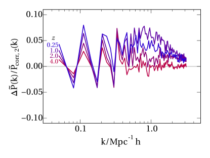
Figure 5: Finite-box errors in power spectrum estimates can be vastly reduced using a paired simulation. Here we show our correction for the next-to-leading-order error term $\Delta\tilde{P}(k)=\tilde{P}(k)_{\mathrm{corr,2}}-\tilde{P}(k)_{\mathrm{corr,1}}$ as a fraction of $\tilde{P}(k)_{\mathrm{corr,2}}$. Despite having a reasonable $200\,h^{-1}\,\mathrm{Mpc}$ box size, correlated artefacts from the small number of large-scale modes propagate down to create an apparent bias in the power spectrum, reaching $\simeq\,5\%$ on scales as small as $k=1\,\mathrm{Mpc}^{-1}h$ at $z=1$. This cannot be corrected by older techniques that divide out cosmic variance in the linear power, as it is an inherently non-linear effect.

As a final example application of paired simulations, we turn to a more immediately practical question. Since numerical simulations of non-linear structure formation can probe only a finite dynamic range, practitioners need to balance the box size against the ability to resolve small scales. The finite volume has two effects: first, it removes all power below $k_{\mathrm{min}}=2\pi/L_{\mathrm{box}}$, where $L_{\mathrm{box}}$ is the comoving size of the box Li et al. (2014). This could be tackled in a computationally-efficient way by assuming a separate-universe approximation and rescaling the background cosmology in each “patch” Angulo and White (2010); we will not consider this further here. The second effect of the small box is that it samples only a small number of modes for wavenumbers reaching $k=k_{\mathrm{min}}$, leading to variance effects that vanish in a true ensemble mean. Paired simulations can be helpful in tackling this problem.

In this section we will need to make a clear distinction between the theoretical power spectrum $P(k)$, as defined by Eq. (3), and the measured power spectrum $\tilde{P}(k)$ which is defined with reference to the discretized density field components in a simulation

$$\tilde{P}(k)=\frac{1}{N_{k}}\sum_{i\in S_{k}}\delta_{i}^{*}\delta_{i}\,,$$ (12)

where $\delta_{i}$ is the density field Fourier component with index $i$, $S_{k}$ is the set of such components that are used in the power spectrum estimate for wavenumber $k$, and $N_{k}$ is the size of that set. Shot-noise corrections Jing (2005) can be applied to Eq. (12) without changing the discussion; we omit it for simplicity. Expanding $\delta_{i}$ to second order in perturbation theory, we have

$$\tilde{P}(k)\simeq\frac{1}{N_{k}}\sum_{i\in S_{k}}\left(\delta_{i,L}^{*}\delta_{i,L}+G_{ijk}\left(\delta_{j,L}^{*}\delta_{k,L}^{*}\delta_{i,L}\right)+\mathrm{c.c.}+\cdots\right)$$ (13)

where $\delta_{i,L}$ is the linear amplitude for component $i$, c.c. indicates the complex conjugate of the preceding term, $D$ is the linear growth factor, and $G_{ijk}$ describes how mode $i$ grows in response to the amplitude of modes $j$ and $k$, evaluated at a given redshift. The linear growth function has been absorbed into the definition of the linear field according to Eq. (4). There is an assumed summation over all modes $j$ and $k$.

Given simulations of a specified box size, the ideal quantity to calculate is $\langle\tilde{P}(k)\rangle$, i.e., an average over all possible realizations of the initial field $\delta_{i,L}$. This is typically attempted by computing tens or even hundreds of realizations Heitmann et al. (2010, 2014), which is computationally costly. The leading-order correction that this generates compared to a single realization can actually be applied by hand, since $\langle\tilde{P}(k)\rangle=P_{L}(k)+\cdots$. The required “first-order corrected” power spectrum estimate is

$$\tilde{P}(k)_{\mathrm{corr,1}}=\tilde{P}_{AA}(k)+P_{L}(k)-\tilde{P}_{LL}(k)\,\textrm{,}$$ (14)

so that $\tilde{P}(k)_{\mathrm{corr,1}}-\langle\tilde{P}(k)\rangle$ is third order in $\delta$. Note that this is different from the usual approach of “canceling” sample variance Springel et al. (2005) by estimating

$$\tilde{P}(k)_{\mathrm{corr,std}}=\tilde{P}_{AA}(k)\frac{P_{L}(k)}{\tilde{P}_{LL}(k)},$$ (15)

which is hard to justify from a theoretical point of view (though one gets the right answer on linear scales by construction).

With a paired simulation in hand, we can go further and apply the next-to-leading-order correction because, inspecting Eq. (13), the error has odd parity in $\delta_{L}$ and so reverses sign in $P_{BB}$. Thus,

$$\tilde{P}(k)_{\mathrm{corr,2}}=\frac{1}{2}\left(\tilde{P}_{AA}(k)+\tilde{P}_{BB}(k)\right)+P_{L}(k)-\tilde{P}_{LL}(k)\textrm{.}$$ (16)

Residual errors in $\tilde{P}(k)_{\mathrm{corr,2}}$ compared to $\langle\tilde{P}(k)\rangle$ are then fourth order in $\delta$.

The corrections arising from this change are highly significant in the case of a $200\,h^{-1}\,\mathrm{Mpc}$ box. Figure 5 shows the correction $\Delta\tilde{P}(k)=(\tilde{P}_{BB}(k)-\tilde{P}_{AA}(k))/2$, as a fraction of $\tilde{P}(k)_{\mathrm{corr,2}}$. The corrections reach $\sim\,5\%$ even at small scales, $k=1.0\ h^{-1}\mathrm{Mpc}$, and modest redshifts, $z=1$, where one might hope the box size effects to be minimal. This is consistent with what is found by averaging over hundreds of realizations (Heitmann et al., 2014) or comparing to increased box sizes which better sample the large-scale modes (Schneider et al., 2015).

Moreover, unlike the second-order cosmic variance, the third-order error is strongly correlated over different $k$’s, presumably because it arises from the coupling to a small number of low-$k$ modes Meiksin and White (1999). In other words, the sample variance is not determined solely by the number of modes in the initial conditions at the same wavenumber, but can instead be dominated by the $G_{ijk}$ coupling to the poorly-sampled low-$k$ modes.

By performing just one additional simulation, it is possible to remove this bias to third order accuracy. The fourth-order term is left invariant by the averaging. Overall, our paired technique enables significant gains in computational efficiency when generating non-linear power spectra for comparison with large cosmological surveys.

III Extensions

Figure 6: As an example extension, we show the cross-correlation between the spliced (“S”) simulation and the original (“A” and “B”) pair. Modes in the S initial conditions are equal to the “A” modes on small scales ($k>0.5\,\mathrm{Mpc}^{-1}\,h$), but to the “B” modes on large scales ($k<0.5\,\mathrm{Mpc}^{-1}\,h$). In cross-correlation with the A simulation, one sees the effect of large-scale streaming decorrelating the small scales. Conversely, the lower panel shows a trend towards coherence between S and B simulations on small scales, showing that the final power at large $k$ is being sourced by low-$k$ density fluctuations. All three simulations have a $\Lambda$CDM power spectrum, so the effects are being directly measured within a realistic cosmological setting rather than a toy model.

As well as fleshing out the three applications in Section II, future work could examine wider classes of statistics-preserving transformations; for example, anything of the form

$$\delta(\bm{\mathbf{k}})\to T(\bm{\mathbf{k}})\delta(\bm{\mathbf{k}})$$ (17)

with $|T(\bm{\mathbf{k}})|^{2}=1$ is suitable. For the overdensity field to remain real, one additionally requires $T(\bm{\mathbf{k}})=T(-\bm{\mathbf{k}})^{\star}$ but otherwise there are no restrictions. In particular there is no requirement for $T$ to be isotropic or homogeneous.

Condition (17) ensures that the power spectrum is unchanged; our method of cross-correlation will then allow the study of structure growth in the presence of the correct cosmological background. The form of $T(\bm{\mathbf{k}})$ is dictated by the specific aspect of structure growth under study.

Section II’s A-B simulations correspond to the simplest case of $T(\bm{\mathbf{k}})=-1$; as another example, a translation $\bm{\mathbf{x}}\to\bm{\mathbf{x}}+\Delta\bm{\mathbf{x}}$ corresponds to the case $T(\bm{\mathbf{k}})=e^{i\bm{\mathbf{k}}\cdot\Delta\bm{\mathbf{x}}}$. Let us briefly consider one further illustrative extension, given by

$$T(\bm{\mathbf{k}})=1-2\Theta\left(k_{0}-|\bm{\mathbf{k}}|\right)\textrm{,}$$ (18)

where $\Theta$ is the Heaviside step function. The resulting transformation flips the sign of $\delta$ for wavenumbers below a critical $k_{0}$. We can refer to the simulation resulting from the new initial conditions as ‘spliced’ (abbreviated to S) since the initial conditions are identical to $A$ for $k>k_{0}$ and to $B$ for $k<k_{0}$. In terms of perturbation theory, this splicing operation is more complex than a $k$-independent transformation because it breaks loop terms into an infrared and ultraviolet part with different signs. Being able to segregate parts of loop integrals fully within a numerical simulation in principle allows a very detailed comparison with perturbation theory. Here we will consider only the qualitative results.

Because the S and A simulations are anticorrelated on large scales, the low-$k$ modes destroy the high-$k$ correlations over time (Fig. 6, top panel) just as with the A-B cross correlation (Fig. 3, lower panel). On the other hand, cross-correlating S with B reveals that the low-$k$ modes remain positively correlated at all times, showing that the anticorrelation on small scales does not affect the larger scales. Furthermore, as non-linear power grows in the late-time universe, the ratio $P_{SB}/P$ ultimately becomes positive at large $k$: structure growth is coherent between the S and B universes because it is regulated by the largest scale modes. A full understanding of the coupling of large- and small-scale modes is necessary for distinguishing the bispectrum due to non-linear evolution Wagner et al. (2015) from any primordial contribution. Using our technique this behavior is exposed to quantitative study without ever changing the power spectrum away from $\Lambda$CDM, and with just three simulations rather than expensive averages over large numbers Meiksin and White (1999).

One could expand to an even broader class of transformations where two independent, uncorrelated initial realizations ($\delta_{\mathrm{I}}$ and $\delta_{\mathrm{II}}$, say) are available:

$$\delta(\bm{\mathbf{k}})\to T(\bm{\mathbf{k}})\delta_{\mathrm{I}}(\bm{\mathbf{k}})+S(\bm{\mathbf{k}})\delta_{\mathrm{II}}(\bm{\mathbf{k}})$$ (19)

where $|T(\bm{\mathbf{k}})|^{2}+|S(\bm{\mathbf{k}})|^{2}=1$. This includes another interesting special case where the $k<k_{0}$ modes are kept fixed while $k>k_{0}$ modes are randomized (rather than anticorrelated). This specialization has been studied elsewhere Aragon-Calvo (2012) to average away stochastic fluctuations in halo spin alignments Aragon-Calvo and Yang (2014) and local bias measurements Neyrinck et al. (2014), using large numbers of runs with independent $\delta_{\mathrm{II}}$ fields. Our approach of pulling out information from a single additional simulation with transformed initial conditions could also be applied to this specialization, for example as another way to isolate the contribution of specific $k$ modes to the perturbation theory loop terms.

IV Conclusions

We have introduced the technique of “paired” simulations. We run two simulations (“A” and “B”) that are identical except for having inverted initial linear overdensities ($\delta_{A}=-\delta_{B}$). Since by definition the linear field is symmetric about zero, the two simulations have identical statistical properties. We illustrated how this can be used to better understand the evolution of voids; extract information on the physical basis of perturbation theories; and eliminate a class of finite-volume effects from power spectrum estimates with greater efficiency than existing techniques. Extensions to a broader class of transformations of the initial density field could further enhance the power of this technique.

Appendix A AB cross-correlations in the Zel’dovich approximation

In this Appendix, we derive the result quoted in the text for the cross-power spectrum of the A and B simulations in the Zel’dovich approximation. Our approach closely follows that of previous works Taylor and Hamilton (1996); Matsubara (2008), but extends to the cross-power spectrum with an alternative resummation that we will describe in due course.

The Zel’dovich approximation is the linear-order solution to Lagrangian perturbation theory. The central quantity is the displacement field $\bm{\mathbf{\Psi}}(\bm{\mathbf{q}})$ which describes the movement of particles from their initial positions $\bm{\mathbf{q}}$ to their final position $\bm{\mathbf{x}}=\bm{\mathbf{q}}+\bm{\mathbf{\Psi}}(\bm{\mathbf{q}})$. All information about the system is then expressed in terms of $\bm{\mathbf{\Psi}}(\bm{\mathbf{q}})$. For example, the local density is

$$\rho(\bm{\mathbf{x}})=\bar{\rho}\left|\frac{\mathrm{d}^{3}\bm{\mathbf{q}}}{\mathrm{d}^{3}\bm{\mathbf{x}}}\right|\textrm{,}$$ (20)

where $|\mathrm{d}^{3}\bm{\mathbf{q}}/\mathrm{d}^{3}\bm{\mathbf{x}}|$ denotes the Jacobian determinant of the transformation between Lagrangian and Eulerian coordinates $\bm{\mathbf{q}}$ and $\bm{\mathbf{x}}$, and $\bar{\rho}$ is the volume-averaged density. This allows the fractional overdensity in Fourier space, $\delta(\bm{\mathbf{k}})$, to be written

$$\delta(\bm{\mathbf{k}}) \equiv\int\mathrm{d}^{3}\bm{\mathbf{x}}\,\left(\frac{\rho(\bm{\mathbf{x}})}{\bar{\rho}}-1\right)\,e^{-i\bm{\mathbf{k}}\cdot\bm{\mathbf{x}}}$$

$$=\int\mathrm{d}^{3}\bm{\mathbf{q}}\,e^{-i\bm{\mathbf{k}}\cdot\bm{\mathbf{q}}}\left[e^{-i\bm{\mathbf{k}}\cdot\bm{\mathbf{\Psi}}(\bm{\mathbf{q}})}-1\right]\textrm{,}$$ (21)

where expression (20) has been used to transform the integration variable to $\bm{\mathbf{q}}$ for the first term, whereas the second term has been rewritten with a relabeling of the integration coordinate from $\bm{\mathbf{x}}$ to $\bm{\mathbf{q}}$. Mass conservation demands that $\langle\delta(\bm{\mathbf{k}})\rangle=0$ which, combined with Eq. (21), implies

$$\int\mathrm{d}^{3}\bm{\mathbf{q}}e^{-i\bm{\mathbf{k}}\cdot\bm{\mathbf{q}}}\langle e^{-i\bm{\mathbf{k}}\cdot\bm{\mathbf{\Psi}}(\bm{\mathbf{q}})}\rangle=\int\mathrm{d}^{3}\bm{\mathbf{q}}e^{-i\bm{\mathbf{k}}\cdot\bm{\mathbf{q}}}\textrm{,}$$ (22)

a result that we will use momentarily.

The cross-power spectrum $P_{XY}(k)$ between fields $X$ and $Y$ is defined by

$$\langle\delta_{X}(\bm{\mathbf{k}})\delta_{Y}(\bm{\mathbf{k^{\prime}}})\rangle=(2\pi)^{3}\delta^{D}(\bm{\mathbf{k}}+\bm{\mathbf{k}}^{\prime})P_{XY}(k)\textrm{,}$$ (23)

where $\delta^{D}$ is the Dirac delta-function. Substituting two copies of expression (21) into this definition gives the following expression for the cross-power in terms of the displacement fields:

$$P_{XY}(k)=\int\mathrm{d}^{3}\bm{\mathbf{r}}\,e^{-i\bm{\mathbf{k}}\cdot\bm{\mathbf{r}}}\left[\left<e^{-i\bm{\mathbf{k}}\cdot\Delta\bm{\mathbf{\Psi}}}\right>-1\right],$$ (24)

where we have used Eq. (22) and defined $\Delta\bm{\mathbf{\Psi}}\equiv\bm{\mathbf{\Psi}}_{X}(\bm{\mathbf{q}})-\bm{\mathbf{\Psi}}_{Y}(\bm{\mathbf{q}}^{\prime})$ with $\bm{\mathbf{r}}\equiv\bm{\mathbf{q}}-\bm{\mathbf{q}}^{\prime}$.

The treatment to this point has been exact (up to shell crossing). We now introduce the perturbative element by employing the Zel’dovich approximation, in which the displacement is related to the linear-theory density field $\delta_{L}(\bm{\mathbf{k}})$ by

$$\bm{\mathbf{\Psi}}_{X}^{\mathrm{zel}}(\bm{\mathbf{k}})=i\alpha_{X}\frac{\bm{\mathbf{k}}}{k^{2}}\delta_{L}(\bm{\mathbf{k}})$$ (25)

for a constant $\alpha_{X}$ depending on which field $X$ we consider. For the A field, $\alpha_{A}=1$; for the B field, $\alpha_{B}=-1$.

We additionally want to be able to calculate the cross-correlation $P_{AL}$ between the true and linearly-evolved fields. Since the Zel’dovich approximation and linear theory have to agree in the limit of small density variations, we can represent the linear theory by multiplying the displacements by some small number $\alpha_{L}\ll 1$, but then dividing the output density field (21) by the same small number $\alpha_{L}$. One can think of this procedure as rescaling the input linear field by a growth factor appropriate for some very early time, then undoing the scaling in the final expression. As a verification, we can re-calculate the linear field from Eq. (21), substituting (25) and then Taylor expanding in $\alpha_{L}$:

$$\delta^{\mathrm{zel}}_{L}(\bm{\mathbf{k}}) \simeq\frac{1}{\alpha_{L}}\int\mathrm{d}^{3}\bm{\mathbf{q}}\,e^{-i\bm{\mathbf{k}}\cdot\bm{\mathbf{q}}}\int\frac{\mathrm{d}^{3}\bm{\mathbf{k}}^{\prime}}{(2\pi)^{3}}\alpha_{L}\frac{\bm{\mathbf{k}}\cdot\bm{\mathbf{k}}^{\prime}}{\bm{\mathbf{k}}^{\prime 2}}\delta_{L}(\bm{\mathbf{k}}^{\prime})e^{i\bm{\mathbf{k}}^{\prime}\cdot\bm{\mathbf{q}}}$$

$$=\delta_{L}(\bm{\mathbf{k}})\textrm{,}$$ (26)

confirming the recovery of the linear density field.

We now return to Eq. (24) and insert expression (25) for the displacement fields. In the Zel’dovich picture, $\bm{\mathbf{\Psi}}_{X}$ is always Gaussian, so we can apply the cumulant expansion $\left<e^{-G}\right>=\exp\left[-\frac{1}{2}\left<G^{2}\right>\right]$. We divide the final expression by $|\alpha_{X}\alpha_{Y}|$; for $\alpha_{A}=1$ and $\alpha_{B}=-1$ this has no effect, whereas for $\alpha_{L}\ll 1$ this captures the shift to linear theory described above. Put together, we obtain the following expression for auto- and cross-spectra:

$$P^{\mathrm{zel}}_{XY}(k)=\frac{1}{\left|\alpha_{X}\alpha_{Y}\right|}\int\mathrm{d}^{3}re^{-i\bm{\mathbf{k}}\cdot\bm{\mathbf{r}}}\left[e^{-(\alpha_{X}-\alpha_{Y})^{2}I(\bm{\mathbf{k}},0)/2+\alpha_{X}\alpha_{Y}J(\bm{\mathbf{k}},\bm{\mathbf{r}})}-1\right]$$ (27)

where $I(\bm{\mathbf{k}},\bm{\mathbf{r}})$ captures the effect of the displacement field for two points at distance $\bm{\mathbf{r}}$ on a Fourier mode with wavevector $\bm{\mathbf{k}}$ and is given by

$$I(\bm{\mathbf{k}},\bm{\mathbf{r}})=\int\frac{\mathrm{d}^{3}\bm{\mathbf{k}}^{\prime}}{(2\pi)^{3}}\frac{(\bm{\mathbf{k}}\cdot\bm{\mathbf{k}}^{\prime})^{2}}{k^{\prime 4}}\cos(\bm{\mathbf{k}}^{\prime}\cdot\bm{\mathbf{r}})\,P_{L}(k^{\prime})\textrm{,}$$ (28)

and $J(\bm{\mathbf{k}},\bm{\mathbf{r}})=I(\bm{\mathbf{k}},\bm{\mathbf{r}})-I(\bm{\mathbf{k}},0)$. The exponent in the integral above has two pieces, one that depends on $\bm{\mathbf{r}}$ (proportional to $J(\bm{\mathbf{k}},\bm{\mathbf{r}})$) and the one that does not (proportional to $I(\bm{\mathbf{k}},0)$). The piece that does not depend on $\bm{\mathbf{r}}$ can be pulled out of the integral to generate a $k$-dependent exponential suppression. The exponential for the other piece is expanded to first order and integrated to generate a linear power spectrum term and a harmless $k=0$ correction

$$P^{\mathrm{zel}}_{XY}(k) =e^{-(\alpha_{X}-\alpha_{Y})^{2}(k/k_{\mathrm{NL}})^{2}}\left[P_{L}(k)-I(\bm{\mathbf{k}},0)\delta^{D}(\bm{\mathbf{k}})\right]\textrm{,}$$ (29)

where $k_{\mathrm{NL}}$ is the wavenumber corresponding to a nonlinearity scale, defined by

$$k_{\mathrm{NL}}^{-2} =\frac{1}{2}I(k,0)\,k^{-2}=\frac{1}{12\pi^{2}}\int_{0}^{\infty}P_{L}(k^{\prime})\mathrm{d}k^{\prime}\textrm{.}$$ (30)

It follows that

$$P^{\mathrm{zel}}_{AL}(k) = e^{-(k/k_{\mathrm{NL}})^{2}}P_{L}(k)\,\textrm{, and }$$ (31)

$$P^{\mathrm{zel}}_{AB}(k) = e^{-4(k/k_{\mathrm{NL}})^{2}}P_{L}(k)\,,$$ (32)

which are the results quoted in the main text. The decorrelation scale between the A and B fields is half that of the decorrelation scale between A and L fields, a result confirmed in our measurements from the simulations.

This derivation looks deceptively close to the resummed LPT approach of Ref. Matsubara (2008), which we denote by “M”. However, there is an important conceptual difference in the detail. In Ref. Matsubara (2008), the equivalent of our Eq. (27) is given by

$$P^{\mathrm{zel,M}}_{XY}(k)=\frac{1}{\left|\alpha_{X}\alpha_{Y}\right|}\int\mathrm{d}^{3}re^{-i\bm{\mathbf{k}}\cdot\bm{\mathbf{r}}}\left[e^{-(\alpha_{X}^{2}+\alpha_{Y}^{2})I(\bm{\mathbf{k}},0)/2+\alpha_{X}\alpha_{Y}I(\bm{\mathbf{k}},\bm{\mathbf{r}})}-1\right].$$ (33)

Expressions (27) and (33) are mathematically equivalent: we have just moved a constant from the $\bm{\mathbf{r}}$-independent piece back into the $\bm{\mathbf{r}}$-dependent piece (which we later expand). At infinite order in the expansion this does not matter, but following the same reasoning as above we obtain to the first order in expanded integral,

$$P^{\mathrm{zel,M}}_{AL}(k) = e^{-(k/k_{\mathrm{NL}})^{2}}P_{L}(k),$$ (34)

$$P^{\mathrm{zel,M}}_{AB}(k) = e^{-2(k/k_{\mathrm{NL}})^{2}}P_{L}(k).$$ (35)

The cross-correlation between the initial and final fields is the same, but the AB decorrelation scale differs by a factor of two. The difference can be attributed to re-summation of a different set of operators, demonstrating the fragility of this operation. Equation (27) is constructed such that the perturbative part vanishes for effects arising at small separations, $r\to 0$. This is why it agrees with the intuitive description given in Section II.2 that the AB particle displacement is doubled relative to the AL displacement — this argument implicitly assumes that the displacements are coherent, which only becomes exactly true in the $r\to 0$ (“eikonal”) limit. Conversely, Eq. (33) is ideally suited to expanding the auto-power ($\alpha_{X}=\alpha_{Y}=1$) but has no special properties as $r\to 0$. A more systematic understanding of these differences is beyond the scope of this work.